Abstract
In Ecuador, the implementation of hydroelectric power plants has had a remarkable growth in the energy sector due to its high efficiency, low environmental impact, and opportunities to generate employment. One of the sectors with the greatest benefits from this type of energy has been the rural sector, where several small-scale hydroelectric plants (0.5 MW–10 MW) have been installed, usually with Pelton turbines. Although these turbines are highly efficient, one of the challenges is to obtain the optimal geometry of the bucket to take advantage of the greatest amount of energy from the water, avoiding the separation of the fluid. In this context, this study focuses on the development of an analytical and iterative methodology that allows for the determining of the appropriate dimensions of the buckets to achieve maximum turbine efficiency. For that, a parametric model has been proposed considering the dimensions and main angles of the bucket, the net hydraulic head and the working flow, as well as the power losses. The results of the model have been validated by means of CFD and by contrasting the experimental data obtained from the “Illuchi N2” Hydroelectric Power Plant in Ecuador, and it is concluded that it is possible to improve the turbine efficiency by up to 4%.
1. Introduction
Hydroelectric power plants are an ecological and economical alternative to solving various problems related to energy safety and deficit [1,2,3]. Because of this, hydropower has been widely used both in developed countries such as Canada and Switzerland, as well as in developing countries such as Colombia, Ecuador, and Peru [4,5,6]. In Ecuador, the change of productive matrix has allowed the expansion of these systems promoting economic growth mainly in the rural sector [7,8]. During the last 14 years, small and large-scale hydroelectric projects have been executed as part of the National Energy Efficiency Plan 2016–2035, and today, 62.7% of Ecuador’s total electricity is produced mostly by Francis and Pelton turbines [9,10].
Although the Pelton turbine was invented in the United States in October 1880 by its creator, Lester A. Pelton, not all questions about its design have been answered [11]. Publicly available information on the design method as well as the appropriate geometric shape of turbine buckets remains limited. The situation described, in part, is caused by the high competition in the hydroelectricity business that keeps new information secret [12]. For this reason, the analytical models applied to predict the behavior of turbines in hydroelectric power plants (power generated) present a significative deviation compared to the values measured in situ.
Despite these limitations, various analytical and computational studies have been carried out around the world to provide information on turbine optimization. In this context, Solemslie, in his doctoral thesis, propopsed an experimental and analytical method for the design of the Pelton runner based on the use of Bézier curves [13]. In this study, Solemslie shows that it is possible to achieve a maximum efficiency of 84% by improving the hydraulic geometry of the runner and moving the water jet away from the lip area by 3 [mm] [10]. On the other hand, Suyesh Bhattarai et al., presents a methodology that allows for the incorporation of computational fluid dynamics (CFD) and a triangulation algorithm to optimize the shape of the inner surface of Pelton buckets. To do this, the authors used a model of an existing cube and a group of randomly created surfaces based on perpendicular projections of the water jet that served as the initial population. The results of this simulation using the Smoothed Particle Hydrodynamics computational method showed a 13.21% improvement in the efficiency of the existing model [14].
Regarding optimization by using computational methods, Anagnostopoulos and Papantonis proposed the application of the Fast Lagrangian Simulation (FLS) method for numerical study and the additional Non-Uniform Rational B-Splines (NURBS) method to parameterize the inner surface of the Pelton bucket. They used 12 geometrical parameters for the design of the bucket edge, three more parameters to define the side surface, and an additional parameter to control the bucket radial position. At the end of their study, they concluded that the hydraulic efficiency of a Pelton turbine is mainly affected by its main geometric parameters of buckets such as length, width, and depth; rather than by the shape of its edge or its lateral surface [15]. In the same research line, Vessaz et al. developed a generic methodology to analyze two Pelton runners by using Ansys CFD and FSL. Moreover, the authors carried out an influence study of 11 parameters that define the bucket shape, and concluded that the exit angle, tilt angle, length-to-width ratio, depth-to-width ratio, and pitch diameter have a greater effect on turbine efficiency. The numerical CFX and Fluent results revealed an increase of 6.8% in overall turbine efficiency by reducing the bucket number and by reducing the water exit angle to the lowest possible [16].
Based on previous research, the present work aims to contribute to the development of an analytical methodology to determine the appropriate shape of Pelton buckets to improve overall efficiency. For that, a parametric model has been proposed, taking into consideration velocity triangles, the net hydraulic head, main angles which are part of the bucket, and other important parameters described in recent studies.
2. Case Study: Hydroelectric Power Plant “Illuchi N2”
The Illuchi N2 hydroelectric plant, owned by the public company ELEPCO SA, is one of the main power plants in the north-central area of Ecuador which provides electricity to the cantons of Latacunga, Saquisilí, Pujilí and Salcedo. It is located in the province of Cotopaxi in the Pusuchisí sector, about 9 km from the city of Latacunga, and has been in operation since 1984. This small power plant (see Figure 1) has two Theodore Bell & Cia Pelton-type generation units that use the turbinated waters of the Illuchi 1 Power Plant that is fed by the river that bears the same name. Each generation unit provides 2675 [KW], taking advantage of a gross head of 327 [m] and a flow rate of 0.95 [].
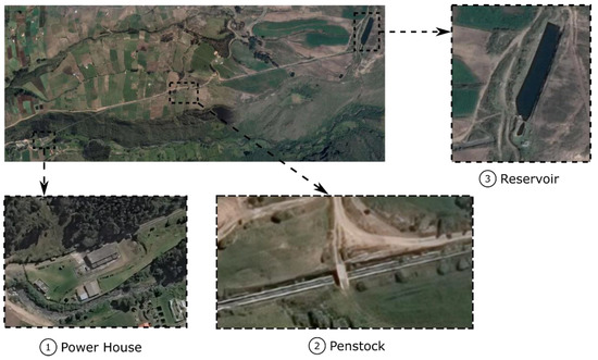
Figure 1.
Hydroelectric Power Plant Illuchi N2.
The rotational speed of both units is 720 [rpm], and they have two synchronous generators composed of five pairs of poles. With these characteristics, the plant contributes to the National Electrification System with a nominal power of 5.20 MW. In Table 1, a summary of the relevant nominal characteristics of each generation unit is presented.

Table 1.
Specifications of the generation units.
3. Theorical Modelling of Pelton Turbine
3.1. Ideal Pelton Turbine Performance
In hydroelectric power plants with Pelton turbines, the available hydropower exists in nature in the form of potential energy. This energy is measured as the geodesic height difference between the upper water level in the reservoir and the turbine shaft in the powerhouse [17]. The transformation of this potential energy into usable mechanical energy for electricity generation is carried out in two stages. In the first stage, the working fluid found in the reservoir is accelerated by passing through the nozzles, thus obtaining kinetic energy in the form of a high-speed jet of water. The rate at which water leaves the nozzle can be estimated using Equation (1), known as Torricelli’s Theorem, that arises from the simplification of Bernoulli’s equation.
In this equation, Vj represents the velocity of the fluid, H is the gross head, g is the acceleration of gravity, and are the losses due to friction and the presence of accessories such as valves, elbows, and forks, among others.
In the second stage, the kinetic energy is transformed into mechanical energy through the interaction of the high-speed water jet with the rotating wheel. In this interaction, the water jet impacts perpendicularly against the divider and is separated into two symmetrical and equal flows that run along the elliptical surface of the buckets modifying their momentum [18]. The shape of the buckets, as well as the path that the water travels, is presented in Figure 2a.
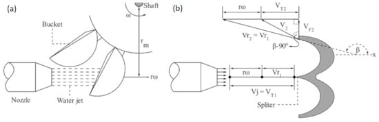
Figure 2.
Pelton buckets schemes: (a) Fluid path in a bucket. (b) Velocity triangles.
Graphically, the interaction described above can be analyzed using the diagram known as velocity triangles. Thereby, it is considered that the rotational speed of the turbine (ω) remains constant and that the only effective force is the impulsive force generated by the water jet. Under these considerations, the input and output of the fluid is analyzed as shown in Figure 2b. Based on this schematic, the velocities tangential to the input and output of the bucket can be determined by Equations (2) and (3), respectively.
From the tangential velocities it is possible to determine the force and torque exerted by the water jet, as well as the mechanical power developed on the turbine shaft. According to classical fluid mechanics, the force exerted by water (F) on the surface of buckets is obtained through the sum of tangential velocities multiplied by the density of the fluid (ρ) and by the flow rate running through the nozzle (Q), as shown in Equation (4) [19].
To find the torque generated on the turbine axis (T), a mathematical term is added to the force equation. This term refers to the perpendicular distance measured from the impact zone of the water jet in the bucket to the turbine shaft. As can be seen in Figure 2a, this distance corresponds to the radius (r), so the torque can be calculated as indicated by Equation (5).
Finally, the power developed on the turbine shaft (P) is quantified through the Equation (6) as the product of torque by the angular velocity at which the wheel rotates.
According to this equation, maximum power is achieved when the linear velocity of the wheel is half the speed of the water jet, and the angle (β) is close to 180°. Figure 3 shows a graph with the theoretical and experimental values of power and torque for a conventional Pelton turbine. In this graph it can be noted that there is a deviation of 15% between the values obtained with the equations and the experimental values. This is because the influence of external factors affecting the behavior of the turbine were not considered for the previous analysis, nor were they considered power losses. However, the equations described provide valuable information and are used to design Pelton turbines at the point of maximum efficiency, known as B.E.P [20].
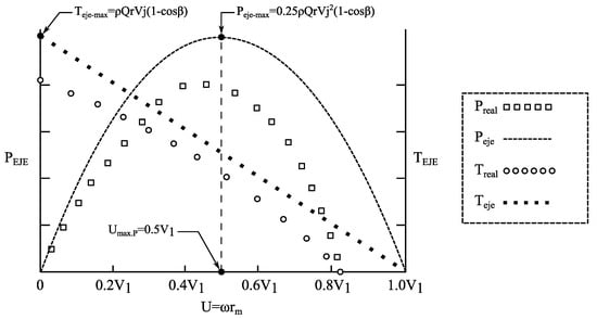
Figure 3.
Power and Torque vs. Rotational Speed.
Although the actual behavior of the Pelton turbine is considerably more complex than assumed above, reasonable results and trends are obtained as presented in Figure 3. To quantify the actual behavior of the turbine it is necessary to include in the analysis the height losses produced in the accelerator nozzle, the hydrodynamic losses caused in the buckets, and the mechanical losses generated between the wheel, casing, and the turbine shaft [21].
3.2. Hydarulic Efficiency
The hydraulic efficiency of a turbomachine is defined as the ratio between the power developed by the wheel and the power supplied by the water jet at the turbine inlet. Mathematically, this efficiency can be found via Equation (7), as the quotient between the specific work of the runner (e) and the specific kinetic energy developed by the water jet [22].
In this equation, the term is known as the peripheral velocity coefficient () and takes a nominal value of 0.50 to 0.47 for the turbine design.
Equation (7) provides a close approximation of the actual hydraulic efficiency; however, it does not consider hydrodynamic phenomena related to swirling losses, friction losses, and water losses [3]. Therefore, certain coefficients must be added to the above equation in order to include such effects in the efficiency estimate. According to Zhang et al. [22], the real hydraulic efficiency of the turbine can be expressed by means of Equation (8)
where () is the peripheral velocity coefficient, is the nominal peripheral velocity coefficient (0.47), () is the degree of reaction of the water jet, and () is the overall friction number. For a Pelton turbine, the degree of reaction and the overall friction number can be determined as shown in Equations (9) and (10), respectively.
where () is the number of buckets, () is the position angle of the buckets, () is the specific speed of the wheel, () is the volumetric load in the bucket, and () is the coefficient of friction, and for calculation purposes it takes a value of 0.015 when the wheel is new and 0.03 when it is eroded. According to the relevant literature, the parameter is given by Equation (14), and it takes the value of 1 when is less than 0.55 [22].
The volumetric load of the bucket, as well as the specific speed of the wheel, can be determined according to the Equations (11) and (12), respectively, which are established as a function of the diameter of the water jet (), the width of the bucket (), the flow rate, () and the number of revolutions (ω) at which the wheel rotates [22].
3.3. Mechanical Efficiency
The mechanical efficiency describes the reduction of power in the turbine due to mechanical losses that occur when the power delivered by the water to the wheel is transmitted to the shaft. The possible mechanical resistances that cause this phenomenon are friction losses with air in the turbine casing () and friction losses in bearings () [23]. These losses are characterized by being dependent on the rotational speed of the turbine and maintain a directly proportional relationship. By combining the effects of both, the mechanical efficiency can be written as Equation (13) indicates.
In Pelton turbines, friction losses with air arise because the remaining air inside the housing generates resistance on the surface of the rotating wheel when set in motion. Based on the IEC60041 standard, these losses for small turbines or horizontal axis turbines can be estimated as a function of the geometric parameters of the casing and the runner, respectively. For that, Equation (14) is used
where is the rotational speed, is the water density, is the gravity value, is the gross head, Q is the flow rate and dimensions are shown schematically in Figure 4.
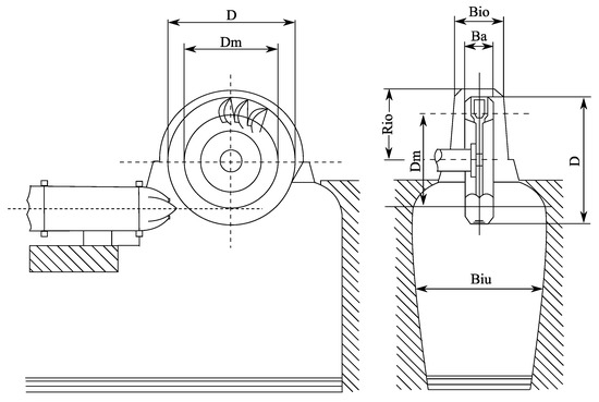
Figure 4.
Pelton turbine casing dimensions.
In addition, the rotational speed can be calculated as the ratio between national electricity frequency (f) to the pole pair number (p) of the synchronous generator by using Equation (15).
On the other hand, the friction losses in bearings () appears when the shear rate of the lubricant increases accordingly with the increased rotational speed, and it depends on the type of bearing used in the shaft of the Pelton Turbine [24]. In general, radial bearings are used for horizontal axis turbines, while axial bearings are used for vertical turbines. As a consequence, is given by Equation (16)
where represents the friction coefficient of each type of bearing and the exponent is equal to 1.5 based on the experiments of Taygun [25].
Another mechanical loss is the friction losses on all shaft seals. Since the shaft seals are not loaded and have a very small sliding surface area, the friction loss on each of them is negligible compared to the losses on loaded bearings. For this reason, they are not considered relevant for the analysis of the mechanical efficiency of the turbine.
3.4. Overall Efficiency of the Pelton Turbine
The overall efficiency of the Pelton turbine is defined as the ratio between the power available on the turbine shaft and the power supplied by the water jet. Algebraically, this efficiency can be expressed as the product of hydraulic, mechanical, and volumetric efficiency, respectively, as presented in Equation (17).
Given that the value of volumetric efficiency () is high compared to the value of other efficiencies, it is often not considered in the analysis of the overall efficiency. Despite this, R. K. Rajput [26] recommends using a value between 0.97 and 0.99 to quantify these losses by volume of water. Consequently, the overall efficiency can be determined as indicated in Equation (18).
From the value of the overall efficiency, it is possible to determine the effective power that the turbine delivers to the electric generator. This power is known as net power on the axis and its numerical value is determined using Equation (19).
4. Parametric Model
The parametric model has been developed considering the parameters and Equations described in the previous sections. As shown in Figure 5, the model is structured systematically in order to estimate the total efficiency and the power on the turbine shaft as a function of the known physical, geometrical and electrical parameters.

Figure 5.
Parametric Model.
5. Validation of Parametric Model
The validation of the parametric model has been carried out both numerically, through a study by computational fluid dynamics, and experimentally, through power and flow rate data obtained by direct measurements in the hydroelectric plant. A detailed description is presented below.
5.1. Numerical Validation
In the absence of experimental measurements, the numerical study by CFD was considered as a first method of validation of the proposed parametric model. This study was carried out using ANSYS 2019 R2 software using the Geometry, Meshing and Fluent modules. The computational domain used in this simulation was obtained from the 3D scan of the runner of the Illuchi N2 Power Plant. This domain is composed of a rotating part named the "rotating domain" and a complimentary a fixed part named the "stationary domain". As can be seen in Figure 6, the domain was simplified from 21 buckets to three and from two nozzles to one in order to reduce the computational cost of simulation. This simplification was performed in order to reduce the computational power according to the method shown by [13].
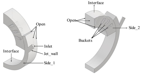
Figure 6.
Computational Domain of Pelton Turbine.
The boundary conditions to carry out the numerical study is summarized in Table 2, considering the current conditions in which the hydroelectric plant operates.
Table 2.
Boundary Conditions for numerical study.
A Cartesian mesh was performed for the discretization process of both the rotating and the stationary domain. Hence, the Cutcell method was used to create regular hexahedra of a defined size. The minimum element size corresponds to 2 mm and the maximum size is 8 mm. As shown in Figure 7, the 2 mm mesh was assigned for the buckets, the 4 mm mesh was used for the water jet walls and the 8 mm mesh was used for the rest of the computational domain. To reproduce the interaction between the static and rotating domains, the “Sliding Mesh Technique” available on ANSYS Fluent was applied. This technique allows for the relative movement of two or more independent meshes along the mesh interface.
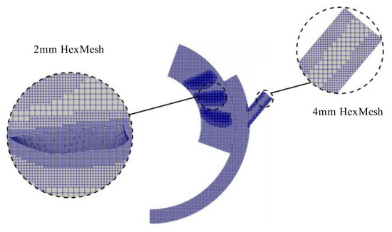
Figure 7.
Discretization of computational fluid domain.
In order to determine the impact of the mesh on the simulation results, a mesh independence study has been performed. Three different meshes (coarse, mid, and fine) were developed and simulated to obtain the most accurate and less computational resources consuming one. Figure 8 shows the convergence of meshes on the torque results. The mid mesh, with 548,926 elements and 579,879 nodes, showed a relative error between the numerical-method resultant torque and the real one of 0.84% and a computing time of 8 h 10 min.
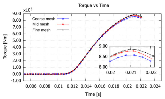
Figure 8.
Mesh dependency.
The efficiency of the turbine depends on the moment generated (torque) by the impact of high-speed water jet that impinges on the runner. For that, a transient state analysis, considering a multiphase model of volumetric fractions of fluid, and a turbulence model k–ε, were used. For the case study, the properties of the fluid were taken at 10 [C], which corresponds to the ambient temperature of the power plant. On the other hand, at the inlet of the computational domain, the velocity-inlet boundary condition was applied with a value corresponding to 80.06 m/s. For the fluid outlet, the pressure-outlet boundary condition was defined with a value of 0 [Pa], and for the buckets, the Wall-rotational boundary condition was used. For the numerical analysis the rotational speed employed is only half the operating speed of the turbine (360 [RPM]). This consideration was applied since in the computational domain only half of the water jet and half of the buckets are used. For the coupling of pressure and velocity, in the Navier Stocks equations the PISO algorithm was applied, and the time step size was 2 × 10⁻⁵ [s] for this analysis. Furthermore, all methods of solution were configured in second order. All of the aforementioned settings (VOF and turbulence model, among others) were obtained from previous studies [14,15,16].
5.2. Experimental Validation
The experimental validation of the parametric model was carried out through the comparison between the calculated values and the values measured in the hydroelectric plant. The data used for validation were the flow, shaft power and efficiency obtained on a normal day of operation of the plant. As shown in Figure 8, the power plant operates between 40% to 100% of the load according to the local electrical demand. The greatest demand for the plant is from 6:00 p.m. to 10:00 p.m. On the other hand, as can be seen in Figure 9, the maximum efficiency reached by the plant at full load is currently close to 90%, and the minimum power at partial load is close to 75%.
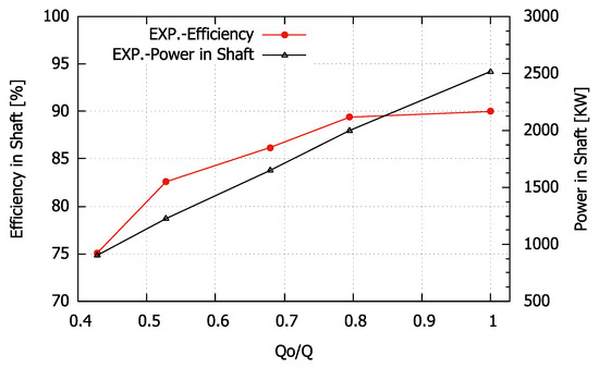
Figure 9.
Effiency and power vs. partial flow rate.
On the other hand, Table 3 presents the values of the different parameters that were used to perform the validation of the model. These values were obtained from the turbine data sheet, the generator data sheet, and the construction drawings of the turbine. For ease of understanding they are ordered as they appear in the model.
Table 3.
Main dimensions and parameters of Illuchi N2 power plant.
6. Optimization Procedure
The optimization process consists of iteratively varying the main geometric parameters of the buckets and determining the maximum overall efficiency achieved with each iteration. As shown in Figure 10, the main parameters are the length of the bucket (L), the width of the bucket (B), and the water exit angle (β).
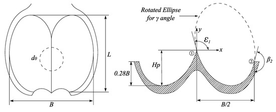
Figure 10.
Main Dimensions of Pelton Buckets.
According to M. Nechleba et.al. [27], these parameters may vary in the range indicated by the correlations shown in Table 4. These correlations allow the empirical determination of the bucket size. It must be stated that these correlations are derived from the geometry of commercially available buckets.
Table 4.
Correlations of Pelton bucket size.
The optimization of the buckets’ geometry continues as follows: the flow rate (Q), net head (H) and the diameter of the nozzles are known values used for the determination of the lineal speed of the water jet (Vj). Likewise, using the number of poles and the value of the national electrical frequency (60 Hz), the rotation speed of the turbine (ω) is determined. From these values, the main coefficients are derived: (i) speed peripherical coefficient (Km), (ii) the volumetric bucket load (φB), (iii)the specific speed (nq), and (iv) the bucket angular position (αo).
To perform the optimization of the buckets through the parametric model, the known values of flow and height are used to determine the speed of the water jet (), as well as the diameter of the water jet for each of the different points of operation of the plant. In parallel, using the number of poles and the value of the national electrical frequency (60 Hz), the rotation speed of the turbine is determined. From the previously calculated values, the main coefficients estimated are the speed peripherical coefficient (), the volumetric bucket load (), the specific speed (), and bucket angular position ().
From these four hydraulic coefficients, the hydraulic efficiency () is determined through Equation (7). An additional parameter appears in this equation, which is called the turbine reaction grade (), and can be found based on the bucket number (), the overall friction number (), and the water exit angle (), which is performed by using Equations (9) and (10). Accordingly, the mechanical efficiency value () can be estimated through Equation (13). Consequently, the windage losses () and friction in the shaft bearings () are calculated through Equations (14) and (16) respectively. In Equation (14), the runner external diameter is computed as , while the other geometrical parameters are taken from the turbine that is currently being analyzed according to Figure 4 and Table 4. After estimating both mechanical and hydraulic efficiency, the parametric model allows for the determination of the overall turbine efficiency (), as shown in Equation (18). At this point, the efficiency value obtained with the previous equations is compared with the value of the overall efficiency measured on the turbine shaft. If the calculated value is greater than the current value, the new power on the shaft is estimated as indicated in Figure 5; otherwise, the geometric parameters related to the shape of the bucket and the casing of the turbine are modified to enhance the overall efficiency value.
7. Results and Discussions
This section comprises a complete analysis of the different outcomes of the methodology presented for a case study that corresponds to the Illuchi N2 hydroelectric plant. First, the results obtained with the parametric model are presented. Afterwards, the numerical and experimental validation of the parametric model is analyzed. Finally, the optimization of the geometry of the buckets is proposed based on four variables, taken as a case study that corresponds to the Illuchi N2 hydroelectric plant.
7.1. Parametric Model Results
Using the data shown in Table 3, the parameters and coefficients needed for the parametric model were estimated. To this end, five points of operation of the hydroelectric power plant were taken into consideration, as shown in Table 5. Consequently, the results obtained from the model are the Overall Efficiency of the turbine and the Power expressed in [KW].
Table 5.
Results of parametric model.
7.2. Numerical Validation of the Parametric Model
The results of the parametric model were validated by CFD according to the methodology proposed in the previous sections. For validation, the moment that the water develops in the walls of the buckets for the different points of operation of the plant, as shown in Figure 11, was estimated.
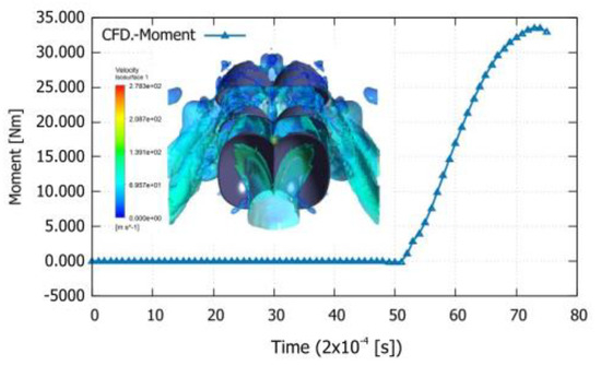
Figure 11.
Moment developed for turbine.
Taking the moment values, the power was estimated according to Equation (20)
where M is the moment developed by the water (torque) on the walls of the buckets and ω is the rotational speed of the turbine in [rad/s]. The results of the numerical study using CFD, as well as the theoretical results, are presented in Table 6.
Table 6.
Theorical and Numerical comparison results.
As can be seen in the table above, the maximum error corresponds to 2.45% when the turbine operates with a partial load of 0.428, while the minimum error corresponds to 0.95% when the turbine operates at full load.
7.3. Experimental Validation of the Parametric Model
In addition to the validation of the parametric model by CFD, validation was carried out with experimental data obtained from the hydroelectric plant. As can be seen in Table 7 and Figure 12, the results obtained theoretically present the same trend as the real data of the plant.
Table 7.
Theorical and experimental comparison.
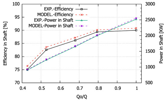
Figure 12.
Experimental Validation.
In addition, the numerical results are comparable to the real ones, presenting a maximum deviation of 1.85% when the plant operates with a partial load of 0.428, and 0.83 when the plant operates at full load. Regarding efficiency, the calculated values show the same increasing trend as the real values. Based on these results, it can be stated that the parametric model developed accurately captures the nature of the phenomenon under study and is suitable for parametric optimization.
7.4. Optimization of the Main Bucket Dimensions
Once the parametric model was validated, the optimization of the dimensions of the buckets was carried out iteratively, as indicated in the previous sections. First, Figure 13 shows the influence of four different β angles, according to the range established in Table 4, with regard to turbine efficiency. The β angles taken for optimization were 160°, 163°, 166° and a maximum of 169°. Although in the indicated range one can take decimal numbers, it was decided to use only integers due to the ease of the construction of the bucket. According to the plot shown, the maximum efficiency value is achieved for a water outlet angle of 169°. When analyzing the influence of this parameter, efficiency increases up to 2%, which is translated into a power increase of 53.94 [KW].
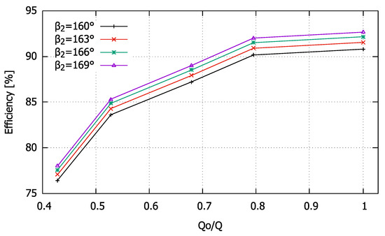
Figure 13.
Influence of Beta angle.
Subsequently, the influence of the width of the bucket (B) on the turbine efficiency was analyzed, following the correlations of Table 4. As presented in Figure 14 four correlations of B as a function of the diameter of the water jet were selected. These relationships are 3.3do, 3.1do, 2.9do and 2.8do. Unlike the previous parameter, a considerable increase in efficiency is obtained. According to Figure 14, an increase of 1.06% of efficiency is achieved by taking the minimum value for the width of the bucket (2.8do). This confers an increase in efficiency of 30.04 [KW].
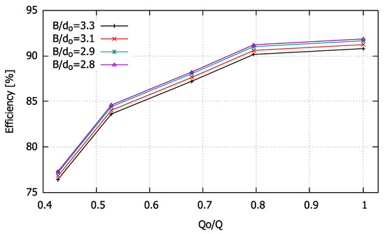
Figure 14.
Influence of B parameter.
In addition, the influence of the length (L) of the bucket on the overall efficiency of the turbine was analyzed. Like the previous parameters, four relationships were selected in the established range (Table 4). The ratios chosen were 2.28do, 2.50do, 3.00do and 3.50do. As can be seen in Figure 15, this parameter has a slight influence on the value of efficiency. However, turbine efficiency can be increased by 0.16% when the minimum value corresponding to 2.28do is used when the turbine operates at full load.
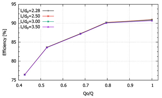
Figure 15.
Influence of L parameter.
The increase in overall efficiency achieved by reducing the width of the bucket and its length is due to the reduction of air friction losses in the turbine housing by achieving a smaller contact surface.
Finally, the influence of the water outlet angle (β), the length of the bucket (L), and the width of the bucket (B) were analyzed together, with which the highest overall efficiency is achieved. As can be seen in Figure 16, by including the three established ratios in the design of the bucket, it is possible to achieve an increase of 3.14% when the turbine operates at full load, an increase of 3.07% when operating at 80% of the total load, and 2.94 when operating at 68% of the total load.
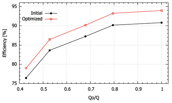
Figure 16.
Optimized Bucket Efficiency.
Regarding the power of the turbine, combining the aforementioned correlations achieves an increase in power equivalent to 88.47 [KW] at full load, as can be seen in Figure 17. In monetary terms, this 3.14% increase in efficiency or 88.47 [KW] represents an income of $55,799.70, considering that the power plant operates 24 h a year with an availability factor of 0.8.
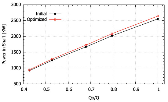
Figure 17.
Optimized Bucket Power.
8. Conclusions
In the present study, a parametric model was developed to quantify the net power on the shaft of a Pelton turbine, considering the hydraulic and mechanical losses present as a result of the operation of the turbine. Based on a thorough validation of the results obtained through CFD and experimental data, it can be concluded that:
The proposed mathematical model satisfactorily reproduces the nature and behavior of the phenomenon under study and can be used to properly define the main dimensions and geometry of the buckets of the wheel of a Pelton turbine.
The parameter that has the greatest influence on the efficiency of the turbomachine under study is the water exit angle (β). By properly defining this value, the efficiency of the turbine may approach 95% when operated at full load.
The width of the bucket (B) maintains an inversely proportional relationship with the overall efficiency of the turbine. This is because by reducing the contact area of the buckets with the rowing air in the turbine housing, the mechanical losses due to friction with the air are reduced and, therefore, the overall efficiency increases.
The length of the bucket (L) has a lesser effect on the overall efficiency of the turbine than the parameters mentioned above. Despite this, it behaves in the same way as the width of the bucket, since a reduction in this value leads to an increase in efficiency.
For the Illuchi N2 Hydroelectric Power Plant case study, it can be concluded that the appropriate dimensions for the bucket design are β = 169°, B/do = 2.8 and L/do = 2.28. With these correlations, an increase in efficiency of 3.14% and a power output of 2643.00 [KW] is achieved. In monetary terms, this increase translates to USD 55,799.70 per year.
Author Contributions
Conceptualization, J.E. and V.H.; methodology, J.E. and M.P.-S.; software, J.E. and G.B.; validation, J.E., V.H. and G.B.; formal analysis, J.E., V.H. and C.T.; investigation, J.E.; resources, V.H. and M.P.-S.; data curation, J.E. and M.C.; writing—original draft preparation, J.E.; writing—review and editing, V.H. and C.T.; visualization, J.E. and G.B.; supervision, V.H. and M.P.-S.; project administration, V.H.; funding acquisition, V.H. All authors have read and agreed to the published version of the manuscript.
Funding
This research was funded by Escuela Politécnica Nacional trough the research project PIGR 20-03.
Acknowledgments
The authors gratefully acknowledge the financial support provided by Escuela Politécnica Nacional through the project PIGR 20-03.
Conflicts of Interest
The authors declare that they have no conflict of interest.
References
- Apergis, N.; Chang, T.; Gupta, R.; Ziramba, E. Hydroelectricity consumption and economic growth nexus: Evidence from a panel of ten largest hydroelectricity consumers. Renew. Sustain. Energy Rev. 2016, 62, 318–325. [Google Scholar] [CrossRef]
- Bhattacharya, M.; Paramati, S.R.; Ozturk, I.; Bhattacharya, S. The effect of renewable energy consumption on economic growth: Evidence from top 38 countries. Appl. Energy 2016, 162, 733–741. [Google Scholar] [CrossRef]
- Ummalla, M.; Samal, A. The impact of hydropower energy consumption on economic growth and CO2 emissions in China. Environ. Sci. Pollut. Res. 2018, 25, 35725–35737. [Google Scholar] [CrossRef] [PubMed]
- Hernández-Gutiérrez, J.C.; Peña-Ramos, J.A.; Espinosa, V.I. Hydro Power Plants as Disputed Infrastructures in Latin America. Water 2022, 14, 277. [Google Scholar] [CrossRef]
- Dia, M.; Shahi, S.K.; Zéphyr, L. An Assessment of the Efficiency of Canadian Power Generation Companies with Bootstrap DEA. J. Risk Financ. Manag. 2021, 14, 498. [Google Scholar] [CrossRef]
- Schmid, B.; Meister, T.; Klagge, B.; Seidl, I. Energy Cooperatives and Municipalities in Local Energy Governance Arrangements in Switzerland and Germany. J. Environ. Dev. 2020, 29, 123–146. [Google Scholar] [CrossRef]
- Vallejo, M.C.; Espinosa, B.; Venes, F.; López, V.; Anda, S. Evading sustainable development standards : Case studies on hydroelectric projects in Ecuador. In Development Banks and Sustainability in the Andean Amazon; Routledge: London, UK, 2019; pp. 175–215. [Google Scholar] [CrossRef]
- Barzola-Monteses, J.; Mite-León, M.; Espinoza-Andaluz, M.; Gómez-Romero, J.; Fajardo, W. Time Series Analysis for Predicting Hydroelectric Power Production: The Ecuador Case. Sustainability 2019, 11, 6539. [Google Scholar] [CrossRef]
- Cruzatty, C.; Jimenez, D.; Valencia, E.; Zambrano, I.; Mora, C.; Luo, X.; Cando, E. A case study: Sediment erosion in francis turbines operated at the san francisco hydropower plant in ecuador. Energies 2022, 15, 8. [Google Scholar] [CrossRef]
- Hidalgo, V.; Díaz, C.; Erazo, J.; Simbaña, S.; Márquez, D.; Puga, D.; Velasco, R.; Mafla, C.; Barragán, G.; Parra, C.; et al. Simplified simulation of a small Pelton turbine using OpenFOAM. IOP Conf. Ser. Earth Environ. Sci. 2021, 774, 012075. [Google Scholar] [CrossRef]
- Quaranta, E.; Trivedi, C. The state-of-art of design and research for Pelton turbine casing, weight estimation, counterpressure operation and scientific challenges. Heliyon 2021, 7, e08527. [Google Scholar] [CrossRef] [PubMed]
- Solemslie, B.W.; Dahlhaug, O.G. A reference Pelton turbine design. IOP Conf. Ser. Earth Environ. Sci. 2012, 15, 032005. [Google Scholar] [CrossRef]
- Solemslie, B.W. Experimental Methods and Design of a Pelton Bucket. 2016. Available online: https://ntnuopen.ntnu.no/ntnu-xmlui/handle/11250/2399557 (accessed on 17 November 2021).
- Gautam, S.; Chitrakar, S.; Neopane, H.P.; Solemslie, W.B.; Dahlhaug, O.G. Numerical investigation of a Pelton turbine at several operating conditions. IOP Conf. Ser. Earth Environ. Sci. 2022, 1037, 012053. [Google Scholar] [CrossRef]
- Židonis, A.; Panagiotopoulos, A.; Aggidis, G.A.; Anagnostopoulos, J.S.; Papantonis, D.E. Parametric optimisation of two Pelton turbine runner designs using CFD. J. Hydrodyn. 2015, 27, 403–412. [Google Scholar] [CrossRef]
- Vessaz, C.; Andolfatto, L.; Avellan, F.; Tournier, C. Toward design optimization of a Pelton turbine runner. Struct. Multidiscip. Optim. 2017, 55, 37–51. [Google Scholar] [CrossRef][Green Version]
- Zhang, Z. Working Principle of Pelton Turbines. In Pelton Turbines; Springer International Publishing: Cham, Switzerland, 2016; pp. 13–28. [Google Scholar] [CrossRef]
- Zhang, Z. Interaction between the Jet and Pelton Wheel. In Pelton Turbines; Springer International Publishing: Cham, Switzerland, 2016; pp. 63–96. [Google Scholar] [CrossRef]
- Mataix, C. Turbomáquinas Hidráulicas Turbinas Hidráulicas, Bombas, Ventiladores; Universidad Pontificia Comillas: Madrid, Spain, 2009. [Google Scholar]
- Rossetti, A.; Pavesi, G.; Cavazzini, G.; Santolin, A.; Ardizzon, G. Influence of the bucket geometry on the Pelton performance. Proc. Inst. Mech. Eng. Part A J. Power Energy 2014, 228, 33–45. [Google Scholar] [CrossRef]
- Çengel, Y.A.; Cimbala, J.M. Fluid Mechanics: Fundamentals and Applications; McGraw Hill: New York, NY, USA, 2014. [Google Scholar]
- Zhang, Z. Hydraulic and Mechanical Efficiency. In Pelton Turbines; Springer International Publishing: Cham, Switzerland, 2016; pp. 207–209. [Google Scholar] [CrossRef]
- Petley, S.; Aggidis, G.A. Estimating the Energy Loss in Pelton Turbine Casings by Transient CFD and Experimental Analysis. Int. J. Fluid Mach. Syst. 2019, 12, 400–417. [Google Scholar] [CrossRef][Green Version]
- Jeon, H.; Park, J.H.; Shin, Y.; Choi, M. Friction loss and energy recovery of a Pelton turbine for different spear positions. Renew. Energy 2018, 123, 273–280. [Google Scholar] [CrossRef]
- Zhang, Z. Power Loss Due to Bearing Frictions. In Pelton Turbines; Springer International Publishing: Cham, Switzerland, 2016; pp. 203–205. [Google Scholar] [CrossRef]
- Rajput, R.K. A Textbook of Hydraulic Machines: Fluid Power Engineering. October 1999. p. 320. Available online: http://www.amazon.com/Textbook-Hydraulic-Machines-Fluid-Engineering/dp/8121916682/ref=sr_1_1?ie=UTF8&qid=1418704471&sr=8-1&keywords=hydraulic+machines+textbook (accessed on 20 June 2022).
- Hydraulic Turbines. Their Design and Equipment. (Translated from the Czech...-Miroslav Nechleba-Google Books. Available online: https://books.google.com.ec/books/about/Hydraulic_Turbines_Their_Design_and_Equi.html?id=5VcKngEACAAJ&redir_esc=y (accessed on 20 June 2022).
Publisher’s Note: MDPI stays neutral with regard to jurisdictional claims in published maps and institutional affiliations. |
© 2022 by the authors. Licensee MDPI, Basel, Switzerland. This article is an open access article distributed under the terms and conditions of the Creative Commons Attribution (CC BY) license (https://creativecommons.org/licenses/by/4.0/).