Article

Site-Adaptation for Correcting Satellite-Derived Solar Irradiance: Performance Comparison between Various Regressive and Distribution Mapping Techniques for Application in Daejeon, South Korea

1
New and Renewable Energy Resource Map Laboratory, Korea Institute of Energy Research, Daejeon 34129, Republic of Korea
2
Energy Engineering, University of Science and Technology, Daejeon 34113, Republic of Korea
*
Author to whom correspondence should be addressed.
Energies 2022, 15(23), 9010; https://doi.org/10.3390/en15239010
Submission received: 28 October 2022 / Revised: 17 November 2022 / Accepted: 22 November 2022 / Published: 28 November 2022

Abstract

:
Satellite-derived solar irradiance is advantageous in solar resource assessment due to its high spatiotemporal availability, but its discrepancies to ground-observed values remain an issue for reliability. Site adaptation can be employed to correct these errors by using short-term high-quality ground-observed values. Recent studies have highlighted the benefits of the sequential procedure of a regressive and a distribution-mapping technique in comparison to their individual counterparts. In this paper, we attempted to improve the sequential procedure by using various distribution mapping techniques in addition to the previously proposed quantile mapping. We applied these site-adaptation techniques on the global horizontal irradiance (GHI) and direct normal irradiance (DNI) obtained from the UASIBS-KIER model in Daejeon, South Korea. The best technique, determined by a ranking methodology, can reduce the mean bias from −5.04% and 13.51% to −0.45% and −2.02% for GHI and DNI, respectively, and improve distribution similarity by 2.5 times and 4 times for GHI and DNI, respectively. Partial regression and residual plot analysis were attempted to examine our finding that the sequential procedure is better than individual techniques for GHI, whereas the opposite is true for DNI. This is an initial study to achieve generalized site-adaptation techniques for the UASIBS-KIER model output.

1. Introduction

A reliable solar resource assessment is important for solar energy projects [1,2,3,4]. In the case of South Korea, various studies on resource assessment have been reported. A feasibility study was performed using ground observation of solar irradiance from the Korean Meteorological Administration (KMA) stations distributed across the country [5]. Despite being the most accurate data, ground observation of solar irradiance with proper quality control availability is limited. As alternatives, satellite data [6,7], reanalysis data used for a feasibility study [8], and typical meteorological year data [3] have been commonly used. The satellite-based solar irradiance model has the advantage of capturing spatial distribution and the dynamic evolution of clouds [9].
In the Korean Peninsula, the University of Arizona Solar Irradiance Based on Satellite-Korea Institute of Energy Research (UASIBS-KIER) model was implemented using the geostationary Communication, Ocean, and Meteorological Satellite (COMS) and GEO-KOMPSAT-2A (GK-2A) satellite imagery to produce solar irradiance estimates from more than 20 years of historical data [6,10,11]. Solar resource potentials have been calculated using the UASIBS-KIER data with good agreement with the ground observation, resulting in a 9.4% normalized mean absolute bias error (MABE). This discrepancy between satellite-derived estimates and observations was also demonstrated in literature for various models [11,12,13,14], leading to a necessary post-processing step to reduce the errors.
Satellite-derived solar irradiance can be corrected through post-processing and combination with ground observation data, which is called “site-adaptation”. Site-adaptation has become an inevitable step for enabling the use of satellite-derived solar irradiance values in the resource assessment process of solar energy projects, such as photovoltaic or concentrating power plants [4]. Site-adaptation techniques have been developed from traditional statistical models such as linear regression [15] to advanced methods such as ensemble model output statistics and various machine learning techniques [16]. Even though the probabilistic site-adaptation method can result in a lower error after correction, it requires several gridded products of solar irradiance. This study will focus on using the single-gridded product of solar irradiance, i.e., the UASIBS-KIER model, which has been designed and validated for South Korea.
The most common methods for site-adaptation are linear regression [17,18] and quantile mapping (QM) [19], owing to their simplicity. There have been variations and improvement to these methods, such as polynomial regression [20], quantile delta mapping (QDM) [19], and polynomial fit of the empirical cumulative distribution function (ECDF) [21]. Nevertheless, it was argued that with these models, the correction of bias can be further improved, hence the sequential method of multilinear regression followed by the quantile mapping technique was proposed [22,23].
The sequential technique aims at correcting the bias in the first step of regression and the distribution correction in the quantile mapping step. It was reported to successfully reduce the mean bias of modeled GHI datasets by more than 20% for datasets with an original bias of >30% in some sites of the Americas, Europe, and Africa regions. However, the distribution mapping method used in the second step was only quantile mapping, while other reports show that other distribution mapping techniques (e.g., using Kernel Density Estimation) could have a better performance [22,24]. Moreover, it was indicated that the application for yet another region is possible and necessary for improvement in the site-adaptation procedure.
This is an initial study that attempts to correct the satellite-derived solar irradiance obtained from the UASIBS-KIER model in Daejeon, South Korea, using site-adaptation techniques. To accomplish this objective, individual and sequential site-adaptation techniques from previous studies were reviewed and then utilized for benchmarking reference. In this paper, considering the potential of other distribution mapping techniques, we expanded the sequential procedure with various distribution techniques. The sequential site-adaptation procedure was performed using a multilinear regression method [22,23] followed by various distribution mapping techniques (QM [19,22,24,25], QDM [19], and polynomial fitting of the ECDF [21]). The site-adaptation performance was then evaluated using error statistics to measure discrepancies, distribution differences, and overall performance. The investigation is followed by a selection of the best technique, using a ranking procedure for determination.
In comparing the performance of various site-adaptation techniques, [22] conducted a benchmarking using three error metrics, but no explicit ranking was provided. Another study proposed a ranking procedure for site-adaptation using seven kinds of metrics [26]. However, they are specified for a case where a polynomial order for regression is to be chosen, for which a direct usage for different cases would require adjustments. A simple approach of using percent values of four metrics and obtaining a new overall ranking was reported for an evaluation of solar irradiance models [27]. While the ranking of each metric might be different, the overall ranking will highlight the model that performs the most consistently for any type of metric. Such a ranking procedure might be practical for ranking various site-adaptation methods in terms of both bias and distribution mismatch reduction. In this paper, a similar ranking methodology is tailored to fit our study which takes into account six types of error statistics.
The datasets employed in this study have been described in Section 2. Section 3 addresses various site-adaptation techniques. Subsequently, Section 4 explains the results from the evaluation by using error statistics and the proposed ranking methodology. The site-adaptation performance is discussed in Section 5, including a comparison between individual and sequential techniques and an analysis of the multi-linear regression technique using partial regression plots and residual plots. Finally, the best method to correct the global horizontal irradiance (GHI) and direct normal irradiance (DNI) in clear- and cloudy-sky conditions is summarized in Section 6.

2. Data

2.1. Satellite-Derived Datasets

In this study, the UASIBS-KIER satellite model [11] was used to derive solar irradiance in Daejeon, South Korea. The UASIBS-KIER model was modified from the UASIBS model [10] for the Korean Peninsula, as shown in Figure 1. The UASIBS-KIER model has been implemented with various satellite imagery, resulting in different time-series product time resolutions [28]. Despite the long temporal coverage of solar irradiance time series (up to 23 years of historical data) [6], the requirements of site-adaptation processes for coincidence quality-controlled ground measurement data limit the time period that can be used. In this study, we used data from 2014 to 2019 where the UASIBS-KIER model used the COMS Level-1B data observed by the Meteorological Imager onboard the COMS satellite over the Korean Peninsula with 15-min temporal resolution.

2.2. Ground-Based Observation

The ground observations were measured at the Korea Institute of Energy Research in Daejeon, South Korea, as indicated in Figure 1; data from 2014 to 2019 were used. The ground observation data were obtained using the Kipp and Zonen model CHP1 pyrheliometers and CMP11 pyranometers for DNI and GHI, respectively. The 1-min data points of the observation data were averaged over 15 min to match the temporal resolution of the corresponding satellite data. To maintain significant short-term variability, more aggregation into a coarser temporal resolution is not performed.
It is important to use highly accurate ground observation data because site-adaptation procedures assume the measurements to have a substantially lower uncertainty than satellite data. Therefore, the instruments and operations must be maintained at a high quality and standard. The observation dataset underwent a quality control test, whose criteria can be found in [28,29]. Data points that did not pass the test were excluded from further analysis. The criteria for quality control are given below:
a.
θ s < 75 °
b.
GHI > 0 ,   DHI > 0 ,   DNI   0
c.
DNI < 1100 + 0.03   h
d.
DNI < S 0 n
e.
DHI < 0.95 S 0 n cos 1.2 h + 50
f.
GHI < 1.50 S 0 n cos 1.2 h + 100
g.
DNI cos θ s + DHI GHI GHI < 0.05
h.
DHI GHI < 1.05   when   GHI > 50   and   θ s < 75 °
i.
DHI GHI < 1.10   when   GHI > 50   and   θ s > 75 °
where θ s , h , and S 0 n denote the solar zenith angle, terrain elevation, and extra-terrestrial irradiance on a normal surface, respectively.

3. Methods for Site Adaptation

After obtaining observation and satellite data for the same period (2014–2019) and the same time resolution (15 min), both datasets were separated into training and test subsets (50:50 ratio). A higher testing subset proportion would mimic the ideal case of site-adaptation that corrects long-term solar irradiance data (test subset) using short-term data (training subset). However, the limited period of high-quality observation data hindered this implementation because the training subset needed to be sufficient to ensure the efficiency of site-adaptation procedures. As demonstrated in [23], a training period of six months or less can lead to erroneous site-adaptation results. Therefore, we attempted to maintain an adequate training period by using the 50:50 training-to-test ratio.
Both the satellite-modeled and observed training subsets were used to obtain the correction factors or functions for site adaptation, which were then used to correct the satellite-modeled test subset, and finally validated against the observed test subset. It is worth noting that the observed values of the test subset were only used to validate the site-adapted results and did not contribute to the correction process.
The site-adaptation methods employed in this study can be categorized into two types of families, namely, regressive and distribution-mapping. Essentially, regressive methods rely on the relationship of each pair of data points. Distribution mapping, however, is used to perform correction after the data points are transformed into a distribution function. Therefore, the correction is based on the distribution of data points, not the data points themselves. After correction, these data points in the form of a distribution are transformed back into time-series data. Owing to this difference, distribution mapping techniques are expected to produce better KSI and OVER in comparison to regressive techniques. Figure 2 illustrates an example of each regressive and distribution mapping site-adaptation technique and Table 1 lists the methods to which they belong, along with the source of the method. In this section, we describe the implementation of each method. Mathematical descriptions for each method can be found in the Supplementary Materials.

3.1. Regressive Methods

The regressive methods used in this study include linear regression (LIN), polynomial regression (POLY), and multilinear regression (MLR). The correction function will be determined by fitting the data points in pairs, between the modeled and observed data in the LIN and POLY methods or between the predictor variables and response variables in the MLR method.
The multilinear regression (MLR) model incorporates several physical parameters that might be best for predicting observed solar irradiance [23]. For GHI, the response variables include the measured clearness index ( k t ), and regression is performed to determine the best combination of these variables, i.e., modeled clearness index, modeled clear-sky index ( k c ), relative air mass, and solar elevation angle. For DNI, it is based on the predicted value of DHI; then, the predicted DNI is calculated using the following equation: GHI   =   DNI cos   θ s + DHI . The observed diffuse ratio ( k d ) is the response variable for DHI MLR; its predictor variables include the relative air mass ( m ), solar elevation angle ( θ e ), modeled clear-sky index, and modeled normalized clearness index.
The best combination of predictor variables is selected by the Akaike information criterion (AIC), which is used as a model to produce site-adaptation results. It should be noted that owing to this step, the model used for MLR site adaptation can be different for each unique condition (i.e., different solar irradiance components, sky conditions, site locations, or time periods).
The relative air mass can be calculated using the formula proposed by [31], which was then corrected by [32]; it represents a function of the solar zenith angle ( z ) and altitude ( h ) of the considered site. Moreover, k t , m was designed to diminish the solar zenith angle dependence of k t by normalizing it with respect to a standard clear-sky GHI profile (normalized to 1 for a relative air mass of (1) [33]. The equations used for MLR are listed below, where TOA represents the top-of-atmosphere solar irradiance on the same plane ( S 0 . cos z ) and CGHI is the clear-sky GHI, which comes from the UASIBS-KIER model.
k t = GHI TOA
k c = GHI CGHI
k d = DHI GHI
k t , m = k t 1.031   exp 1.4 / 0.9 + 9.4 / m + 0.1
m = 1 cos z + 0.50572 · 96.07995 z 1.6364 · exp h 8434.5

3.2. Distribution Mapping Methods

In distribution mapping methods, the correction process starts with transforming the data points into a distribution function. Quantile mapping (QM) is the most common method, based on the inverse transform [19,24], which can be formulated as
x s a t , t e s t , c o r r e c t e d = F o b s , t r a i n 1 F s a t , t r a i n x s a t , t e s t ,
where x is the sorted irradiance value and F x is the probability of finding an irradiance whose value is less than or equal to x .
This method has several variations, such as statistical parameter tuning and improvement, for obtaining the CDF [24]. The parameter tuning involves the selection of the number of quantiles. In this study, the following number of quantiles are employed: ECDF mapping uses N, QM few uses 5, QM some uses N0.5, and QM many uses N/5 number of quantiles, where N denotes the total number of data points. The second variation of this method includes KDE mapping, where the CDF is obtained by integrating the probability density function (PDF) obtained from kernel density estimation.
Quantile delta mapping (QDM) is similar to the QM technique; however, the satellite-derived solar irradiance of the testing dataset is not transformed into the probabilistic profile of the training dataset. Instead, the probabilistic profile of the testing dataset is directly inversely transformed into bias-corrected solar irradiance values; subsequently, it is multiplied by the relative change between the solar irradiance of the testing and training datasets.
x s a t , t e s t , c o r r e c t e d = F o b s , t r a i n 1 F s a t , t e s t x s a t , t e s t × Δ r
Δ r = F s a t ,   t e s t 1 y s a t , t e s t F s a t ,   t r a i n 1 y s a t , t e s t = x s a t , t e s t F s a t ,   t r a i n 1 y s a t , t e s t
Compared with the standard QM, QDM preserves the relative changes between variables in two different time periods; this is to ensure that the long-term trends in all quantiles are preserved. However, in the QM method, they can artificially deteriorate (owing to the transformation of the probability profile of the testing dataset). Although the realistic nature of long-term trends related to natural or climate changes (such as temperature variability) depends on the model, the QDM technique helps in preventing artificial alterations in the trend of the variable of interest during site-adaptation. Lastly, the polynomial fit of ECDF (Polyfit) was used especially with an aim for improving DNI as it is reported to have a better improvement in the direct component in comparison to the global horizontal irradiance [21]. In contrast to the aforementioned methods that are based on the inverse transform, a polynomial fitting is used for both observed and modeled ECDFs. The difference in the fitting coefficients is subtracted to correct satellite-modeled data.

3.3. Sequential Methods

The sequential methods employed in this study expanded the previously proposed procedure, which was employed only for the QM method. MLR is used as the first step, then followed by various distribution mapping methods described in Section 3.2. After the distribution mapping technique, a final check is performed; if the final result is negative, the original modeled values will be used.

4. Results

4.1. Error Statistics

Considering the important aspects for evaluating site-adaptation performance, six metrics are chosen for this study which can be categorized into three types. The first type includes the three common statistics: mean bias error (MBE), mean absolute bias error (MABE), and root mean squared error (RMSE); the percentage values of these statistics were considered after normalizing to the mean of the observation dataset. They are the measure of the difference in each individual pair (between each modeled data point with its respective measured value). RMSE is the most widely used, owing to its high penalty for large errors that are especially undesirable in solar irradiance data [34]. The following equations define the error metrics, where M i denotes the satellite-derived (modeled) value and O i is the observation value, with N total data points:
MBE = 1 N i = 1 N M i O i 1 N i = 1 N O i
MABE = 1 N i = 1 N M i O i 1 N i = 1 N O i
RMSE =   1 N i = 1 N M i O i 2 1 N i = 1 N O i
It is also important for the satellite-derived time series to have a matching frequency distribution to that of the ground-observed data, such as for estimating long-term average data or developing a typical meteorological year [27,35]. This aspect can be measured by the Kolmogorov–Smirnov Integral (KSI) and its pair for overcritical values, OVER [35]. KSI and OVER are the measures of how much two distributions (CDFs) differ from each other. A lower KSI and OVER mean a more similar distribution. KSI can also be a measure of the variability of the solar irradiance data, where low variability is indicated by a large KSI. The minimum value of the KSI is zero, implying that the two datasets can be considered to have a statistically identical distribution. KSI and OVER can be calculated as follows
KSI = 100 A c x min x max D n d x
OVER = 100 A c x min x max ( D n V c )   d x       if   D n > V c 0                                             if   D n V c
V c = Φ N N 1 / 2
where V c is the critical value and Φ N is a function of the number of data points [27]. The calculation of critical value was implemented in our algorithm using the SciPy statistical function “ksone”. As described in [35], the value of OVER is obtained when D n is greater than V c ; in other words, if the value of D n never exceeds V c , OVER is zero.
The last type is the combined index performance (CPI). CPI is the combined performance index that measures both individual-pair and distribution differences, calculated from RMSE, KSI, and OVER. CPI was designed for making a single number comparison amongst several models’ values that are usually similar and thus hard to distinguish [27]. CPI can be defined as follows:
CPI = KSI + OVER + 2 RMSE 4

4.2. Ranking Methodology

The ranking methodology was proposed to compare the site-adaptation performances of the 17 methods used in this study. We aimed to improve the solar irradiance obtained from the UASIBS-KIER satellite model output; hence, it is desirable to find a technique and approach that results in a low error and high distribution similarity, which are denoted by the lowest error metrics (MBE, MABE, and RMSE) and lowest distribution similarity metrics (KSI and OVER), respectively. The overall performance metric, CPI, was also used to measure the performance of the site-adaptation method.
The ranking procedure proposed in this study calculates the overall best of the aforementioned six metrics’ individual ranking. First, the rank of each metric was determined ( r i for i = 1 ,   2 ,   ,   n , where n is the total number of statistical indicators). Then, the rank of each individual metric was summed, and the values were further ranked; in this case, the lowest and highest sums indicated the best and worst ranks, respectively. Table 2 visualizes the ranking procedure for an example case, GHI in an all-sky condition, where the ranking for each metric is denoted by r1 to r6.
In Table 2, the values were approximated to two decimal places for efficiency. However, in the ranking determination, four decimal places were used to ensure that multiple methods were not selected as the best according to the error metrics (MBE, MABE, and RMSE). This shows that some methods resulted in significantly similar error metric values and additionally supports the use of CPI by [27], presenting metrics that could differentiate the performance of similar performing methods.
This method of ranking considers all statistical metrics described in Section 4.1 to be equally important in the mathematical sense. However, in essence, RMSE, KSI, and OVER would be given more weight since they are imposed for the second time in CPI. More weight in these three metrics is considered necessary due to the importance of reducing large errors and considering the variability in the solar irradiance data. Smoother solar irradiance data might obtain a lower RMSE, while in practice, the information on the variability of solar data holds importance for the user in managing the utilities [36]. Hence, a balance between the evaluation of RMSE and KSI is considered a necessity.

4.3. Evaluation of Original Estimates

Before the site-adaptation process, the dataset was separated into two groups based on the sky conditions, i.e., clear and cloudy skies. The clear-sky condition was determined based on the value of the observed clear-sky index, k c , obs , where k c , obs > 0.9 indicated a clear sky. The satellite model outputs for both GHI and DNI, which were separated into clear and cloudy skies, exhibited different statistical metrics, as shown in Figure 3 and Figure 4, respectively.
As evident from Figure 3 and Figure 4, the UASIBS-KIER model exhibited better performance under clear-sky conditions in comparison to cloudy-sky conditions. These results can be attributed to the difficulties involved in estimating the optical properties of clouds in the atmosphere because it is a major attenuating factor of the solar irradiance received on the ground surface. For DNI, the failure in detecting clouds was immediately reflected in large discrepancies between the satellite-modeled and observed values. Meanwhile, for GHI, a fraction of the solar irradiance consists of diffuse components, leading to less severe discrepancies.
In cases where the model successfully detected clouds, the errors were high in comparison to those in clear-sky conditions due to the various complex ways in which clouds alter the incoming solar irradiance (i.e., scattering, absorption, and transmission), and depended on the cloud condition or type. Despite various efforts to calculate the cloud parameters to account for their effect on the value of solar irradiances received on the ground surface, such as cloud optical depth and cloud classification types, it remains challenging to produce accurate estimates, as evident from the relatively poor metrics summarized in Tables S2 and S5.

4.4. Evaluation of Individual Site-Adaptation Techniques

The site-adaptation performance can be evaluated using the statistical metrics of the adapted values. From now, the site-adaptation methods are referred to by their abbreviations. For the regressive techniques, LIN, POLY, and MLR represent linear, polynomial, and multilinear regression, respectively. The distribution mapping techniques are denoted by ECDF, QM, KDE, QDM, and Polyfit for ECDF mapping, quantile mapping, kernel density estimated QM, quantile delta mapping, and polynomial fit of ECDF, respectively. QM is divided into three parts depending on the number of quantiles, indicated by “few”, “some”, and “many”, as explained in Section 3.2.
For the GHI case in the all- and cloudy-sky condition, it can be observed that QM many yielded the highest rank among the individual techniques. MLR exhibited the best performance for clear-sky conditions. Moreover, the result of those three sky conditions for GHI shows that the MLR method can reduce the error metrics (especially RMSE) more in comparison to other methods, but it failed to reduce the distribution profile differences (i.e., KSI and OVER) under cloudy-sky conditions. Therefore, in the all-sky condition, MLR was outperformed by the QM many method, which consistently reduced the errors and distribution profile differences despite the mediocre amount of correction. The ranking of individual methods in the case of GHI was lower than that of sequential methods, which will be discussed in the next section.
For DNI in the all-sky condition, the Polyfit method demonstrated the highest rank, followed by QM many. The Polyfit method was the third best and best in the clear- and cloudy-sky conditions, respectively. The QDM method obtained the best rank among all methods in the clear-sky condition, but it did not perform well in the cloudy-sky condition.
As expected, distribution mapping techniques show better KSI and OVER in comparison to regressive techniques. However, there is an exception in the case of GHI in clear-sky conditions, indicating that regressive techniques can also improve the distribution similarity; moreover, in some cases, they are better than distribution mapping techniques.
Under distribution mapping techniques, the QM category has five methods. The first four methods (ECDF, QM few, QM some, and QM many) have different quantities of quantile parameters. In other words, the comparison between these four methods shows the sensitivity of the QM method to the number of quantiles. KDE is the fifth method in the QM category, wherein the principles of site-adaptation correction are the same as those of the other four, except for the method used to obtain the distribution profile (CDF). In KDE, kernel density estimation is implemented, with a computation process that is relatively longer than that of empirical CDF, with a small effect, if any, on the site-adaptation performance. Comparing the five methods in the QM type with the other two types (QDM and Polyfit), it can be concluded that no method performs significantly better than others. For estimation, the QM type was better for GHI site adaptation, whereas QDM and Polyfit were better for DNI site adaptation.
The site-adaptation methods used in this study fall into the statistical category [15]; they lack physical interpretation, except the MLR method and, to some extent, the QDM method. Statistical methods share the same sole functionality of obtaining the closest value to the observed data points (for regressive techniques) and closest distribution (for distribution mapping techniques), where the difference is in the various ways of achieving it. This variety lies within the technical variations in statistical techniques (refer to Supplementary Materials for a detailed description of each method). In this situation, it is probable that the difference in performance between each method of site adaptation lies in the problem of overfitting or underfitting. The overfitting profiles capture the minutest details, which could also include random errors. These random errors are rarely the same for different events; hence, when the correction is based on these errors, it would lead to erroneous results.
The MLR and QDM methods incorporate physical meaning into their correction methods. In MLR, even though the variables used are selected from extensive lists of generalized linear models using the AIC number [22,23], the variables can have a physical interpretation. The clear-sky index and clearness index are parameters that represent the atmospheric transmittance for solar irradiance. The relative air mass contains information related to the specific sites used by the elevation height input. The solar zenith angle contains information related to the position of the sun and it is correlated with the bias [37]. The QDM method was developed to preserve the changes in each quantile and mean of data [19]; the changes are preserved to ensure that those resulting from external factors (e.g., climate change effects) are not affected by the site-adaptation process.
In this study, the MLR method exhibited exceptional performance in the GHI case under clear-sky conditions; however, it was outperformed by other methods under GHI cloudy-sky conditions and both cases of DNI. This suggests that the MLR method is not the most suitable for correcting solar irradiance when clouds are the dominant factor. Despite this shortcoming, MLR has its advantage in physical interpretation; moreover, it can be site-specific using site elevation information and the best model selection process. Therefore, it is desirable to perform sequential site-adaptation procedures using MLR, followed by distribution mapping.

5. Discussion

5.1. Performance of Sequential Site-Adaptation Techniques

A sequential site-adaptation procedure using MLR, followed by a distribution mapping technique, was proposed and demonstrated in [22,23]. While it successfully improved the statistical metrics, it was only employed for the QM method. Therefore, we expanded it by performing a sensitivity test on the sequential site-adaptation procedure for various distribution-mapping techniques.
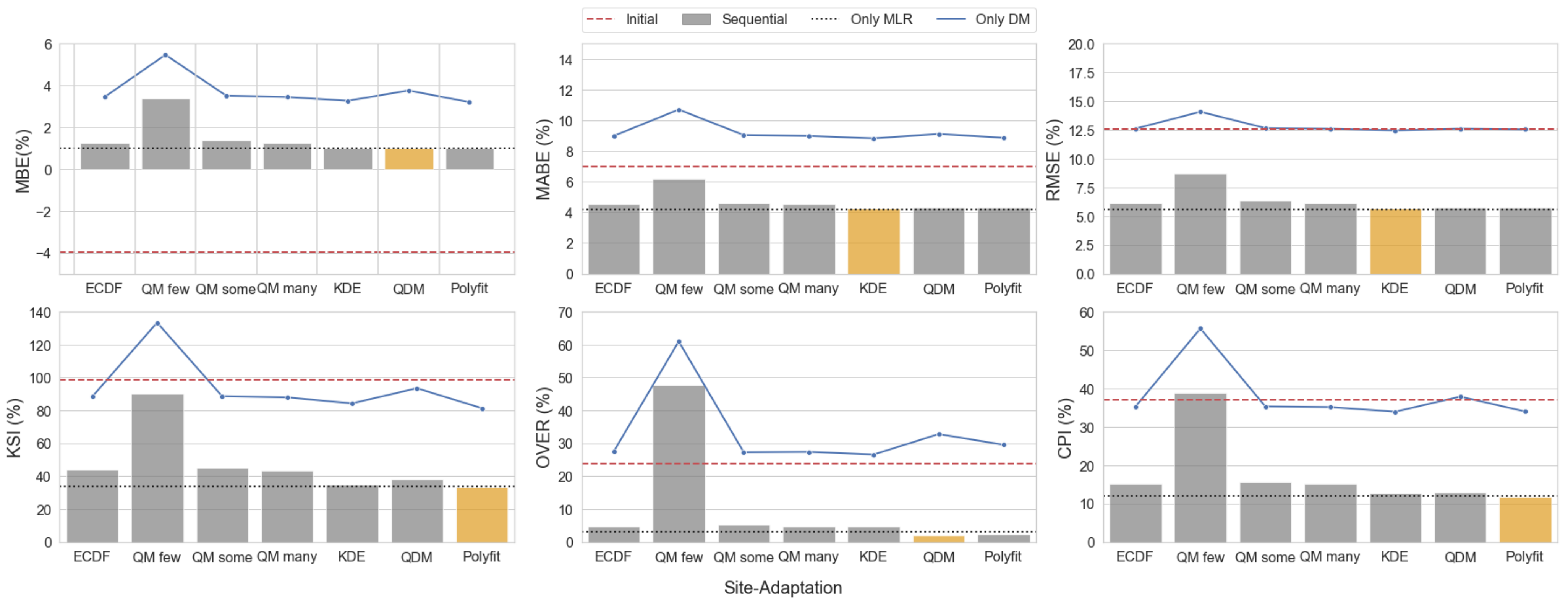
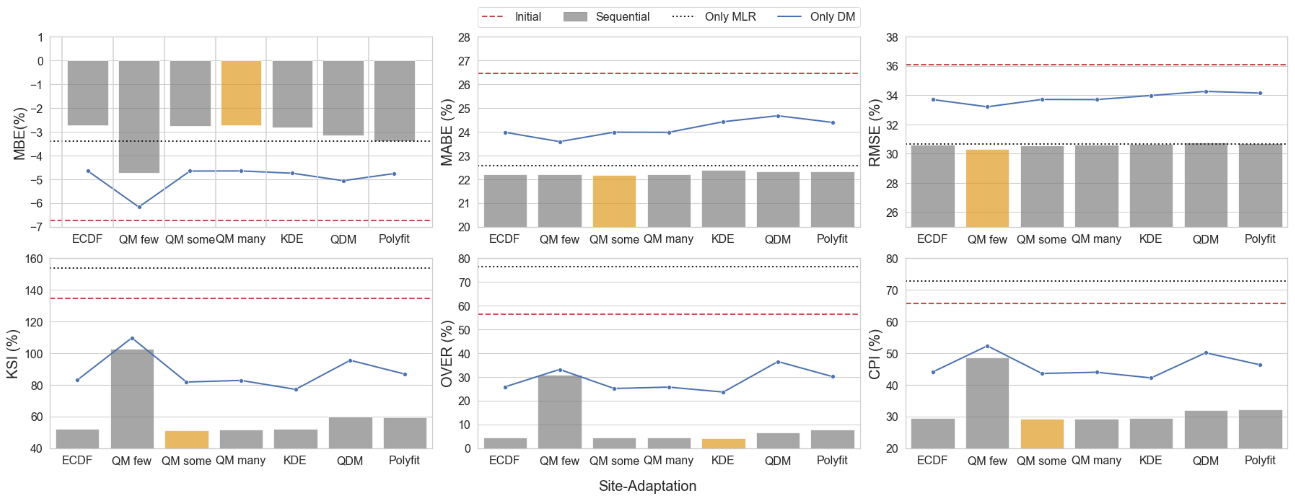
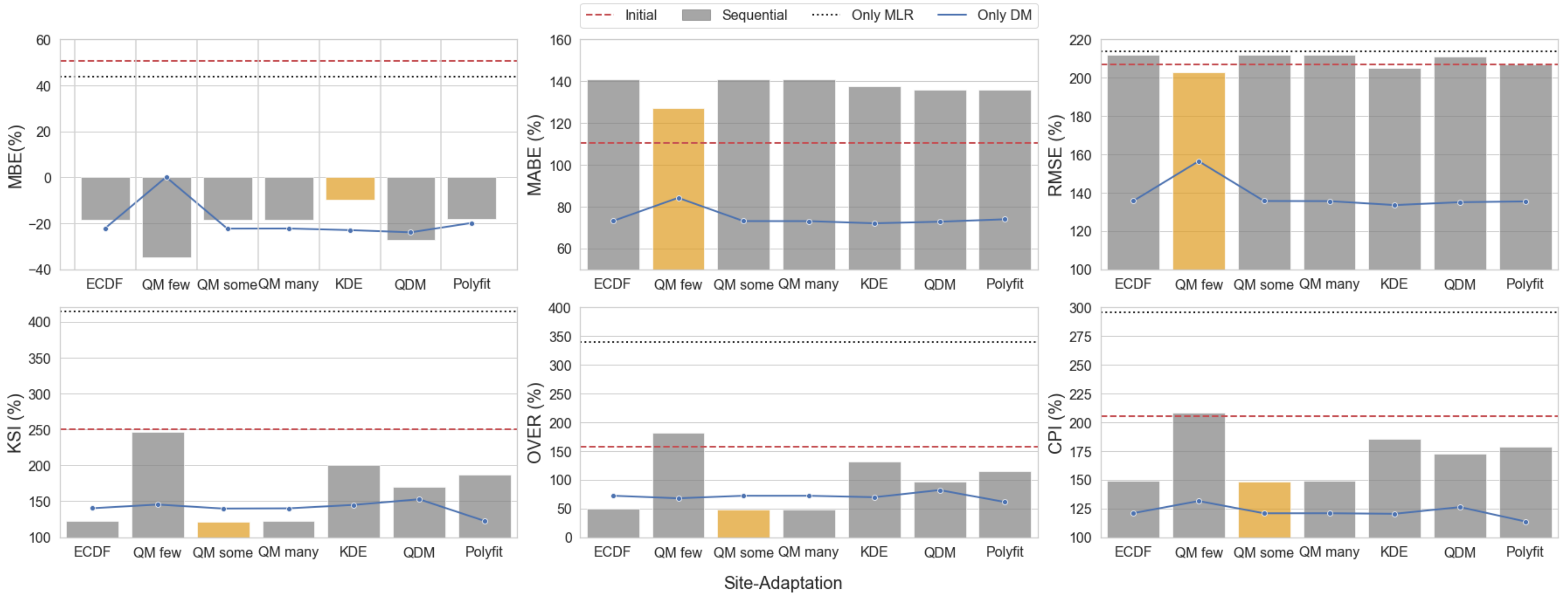
To facilitate the comprehension of sensitivity analysis of distribution mapping techniques, a combination of bar and line plot showing the statistical metrics of each case is illustrated in Figure 5, Figure 6, Figure 7 and Figure 8. The red dashed line, black dotted line, and the blue solid line represent the initial state, results of the MLR method, and individual distribution mapping techniques, respectively; the bar columns represent sequential methods, with the best sequential method (not essentially the best overall method) highlighted in orange.
In the case of GHI, the sequential method procedure improves all individual site-adaptation performances under clear- and cloudy-sky conditions, even when the MLR method results in worse metrics under cloudy-sky conditions. Figure 5 shows the results for GHI under clear-sky conditions. Among the QM techniques that use empirical CDF methods, better results were obtained when the number of quantiles was increased, and the peak performance was achieved by QM many; however, the performance of ECDF became slightly worse (maximum number of quantiles). This might indicate that there is a saturation point for the number of quantiles, i.e., after a certain point, increasing the number of quantiles does not lead to improved site-adaptation performance. In addition to the conventional empirical CDF QM methods, the KDE, QDM, and Polyfit methods exhibited relatively better performances (the best three methods among the sequential methods).
Figure 6 shows the results for GHI under cloudy-sky conditions. Comparing the QM techniques that use the empirical CDF method, peak performance was achieved by QM some, while the performance of QM many and ECDF worsened with small differences; their error metrics were the same up to one decimal point, whereas the distribution similarity metrics were the same to one unit. This finding supports the argument found for the clear-sky condition, i.e., there exists a saturation point of an optimum number of quantiles to be used in the QM method. However, the performance trend between the QM, KDE, QDM, and Polyfit methods differs from that under the clear-sky condition. This complicates the determination of the best method for GHI site adaptation. Overall, compared to individual methods, sequential methods exhibited better site-adaptation performance for GHI.
In the case of DNI, the sequential method resulted in worse metrics in comparison to individual distribution mapping techniques, as described by the overall ranking. Figure 7 and Figure 8 show the results for the clear- and cloudy-sky conditions, respectively. In contrast to the case of GHI, the sequential method was not better than the individual methods in site adaptation for DNI under clear- and cloudy-sky conditions. The individual distribution mapping technique generally performed better in almost all error statistics, particularly MBE, KSI, and OVER. The values of KSI and OVER in the LIN method were similar to those in the initial state but worse in the POLY and MLR methods. Therefore, sequential methods that utilize the MLR method as the first method do not perform well; accordingly, we can conclude that the performance of sequential methods is directly related to the regressive method used in the procedure, which was limited to the MLR method in our study.
In this study, the sequential procedure was worse than the individual method for DNI, whereas the opposite was true for GHI. There are two possible explanations for this behavior. First, this issue may be attributed to the intrinsic difference between GHI and DNI; second, owing to the linear regression problem in the MLR method, the first step of the sequential procedure yielded poor results in the case of DNI.
The UASIBS-KIER model produced estimates for GHI, which were then separated into diffuse and direct components through the Engerer model using the diffuse ratio (kd). Under cloudy-sky conditions, owing to scattering from the clouds, this diffuse ratio could be over 95%, implying that almost all solar irradiance is DHI. Hence, the DNI value was significantly small, if not none, on cloudy-sky days; however, on clear-sky days, the direct component can reach up to 66% [38]. Therefore, the cloud detection model is an important component because false detection can lead to large discrepancies between the actual and modeled data.
Another possible reason is the internal aspect of the MLR method, which demonstrated poor results in the case of DNI, especially in terms of distribution similarity measures (KSI and OVER). In the MLR method, we used the ordinary least squares technique to estimate the coefficients of the regression function, i.e., the estimates depended on the squared error or residuals of each point to the best-fit line. In the scattered plots of observed DNI versus modeled DNI values, owing to the high uncertainty in cloud detection that reflected the determination of DNI (as discussed earlier), some points deviated significantly from the ideal 1:1 line, where the majority of data was located. Therefore, the data points that deviate from the main line would yield a massive squared error or high residuals. These data points could drive the ordinary least squares algorithm to tilt the axis of the fit line to compensate for the high residuals to ensure that the lowest possible total squared error is achieved. This would cause the best-fitted line from linear regression to move away from the line that fits the majority of data (i.e., the fitting line) if there are no high residual data points. Consequently, the predicted values of this model could drift away from the true values, resulting in a poor error and distribution similarity measures. This high residual issue can possibly be addressed by changing the ordinary least squares method to a robust regression model that will weigh down the data points with high residuals or removing the outliers before regression. However, both solutions require meticulous details, which are beyond the scope of this study.
We further analyzed the MLR results for clear- and cloudy-sky conditions for both GHI and DNI by examining the selected best model, its coefficient values, R-squared, and F-statistics. Table 3 summarizes the results of MLR, where var1 to var4 are different for GHI and DNI, as described in Section 3.1. In accordance with the explanation of the MLR method in Section 3.1, it can be observed that the variables used in the model, as well as the intercept and coefficient values, are different for each case. The value of R-squared indicates the capability of the model to explain the changes in the dependent variable, while F-statistics can show whether the groups of variables for our model are statistically significant in explaining the variance of the dependent variable.
Under clear-sky conditions, the choices of independent variables for both GHI and DNI are significant in explaining their respective dependent variables according to the F-statistics. However, the independent variables of DNI and GHI can explain 27.1% and 78.3% of the changes in the dependent variable, respectively. Under cloudy-sky conditions, the choice of independence is also significant for both GHI and DNI according to the F-statistics. The value of R-squared for DNI is also lower than that for GHI, which shows that the DNI and GHI models can explain 34.7% and 58.0% of the changes in the dependent variable, respectively.
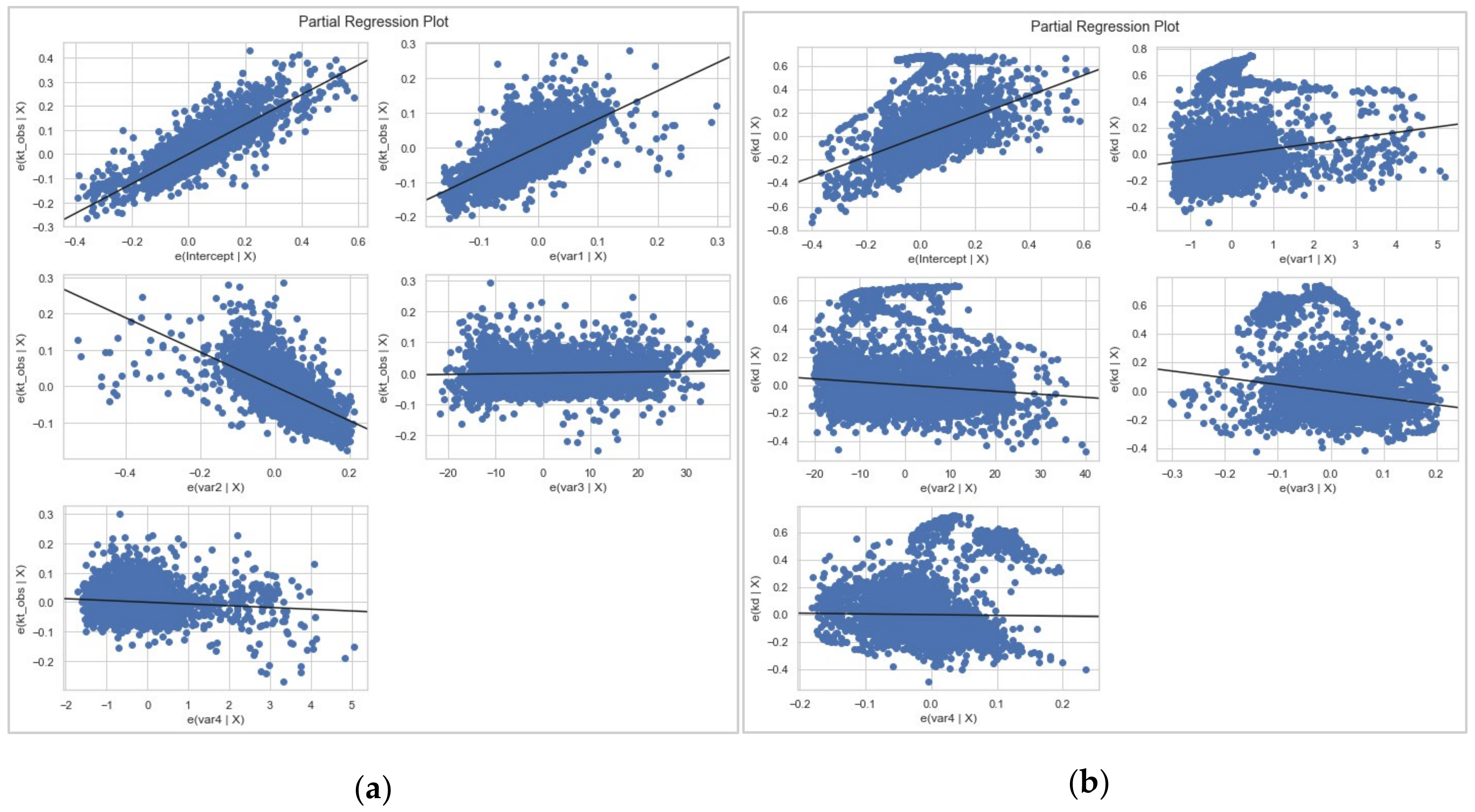
We extended regression analysis by comparing the partial regression plot for each variable in the case of GHI and DNI, as shown in Figure 9. The underlying concept can be traced back to the Frisch−Waugh−Lovell theorem, where the main goal is to reduce the multivariate regression to univariate regression [39,40]. In multivariate regression, individual plots between the response variable versus each predictor variable are not the best way for assessing the effect of each predictor variable on the response variable because it omits the possible correlation among the predictor variables. The partial regression plot helps in determining the correlation between the response variable and i -th predictor variable ( X i ), conditional on other independent variables, and denoted by X ~ i . The x-axis of the partial regression plot is the residual of regressing X i on X ~ i , whereas the y-axis is the residual of regressing the response variable Y on X ~ i .
In the partial regression plot for GHI, relatively strong linear relationships can be observed between the response variable and predictor variables in Figure 9a. In contrast, every partial regression plot in DNI exhibits concerning observations because there are points that lie far from the regression line, which can highly influence the partial relationship between the response variable ( k d ) and predictors. This effect is reflected in the low R-squared value of MLR results for the case of DNI. This issue can be resolved by dropping these points and performing linear regression without them. However, these plots with unusual data points can also be interpreted as being produced due to the selected predictor variables that are not the most accurate at predicting the response variable. Hence, there are data points that do not fit the supposedly linear relationships and are deemed outliers. In the latter case, dropping outliers would be inappropriate because it would be better to find new predictor variables or alternative ways to correlate data, such as binning.
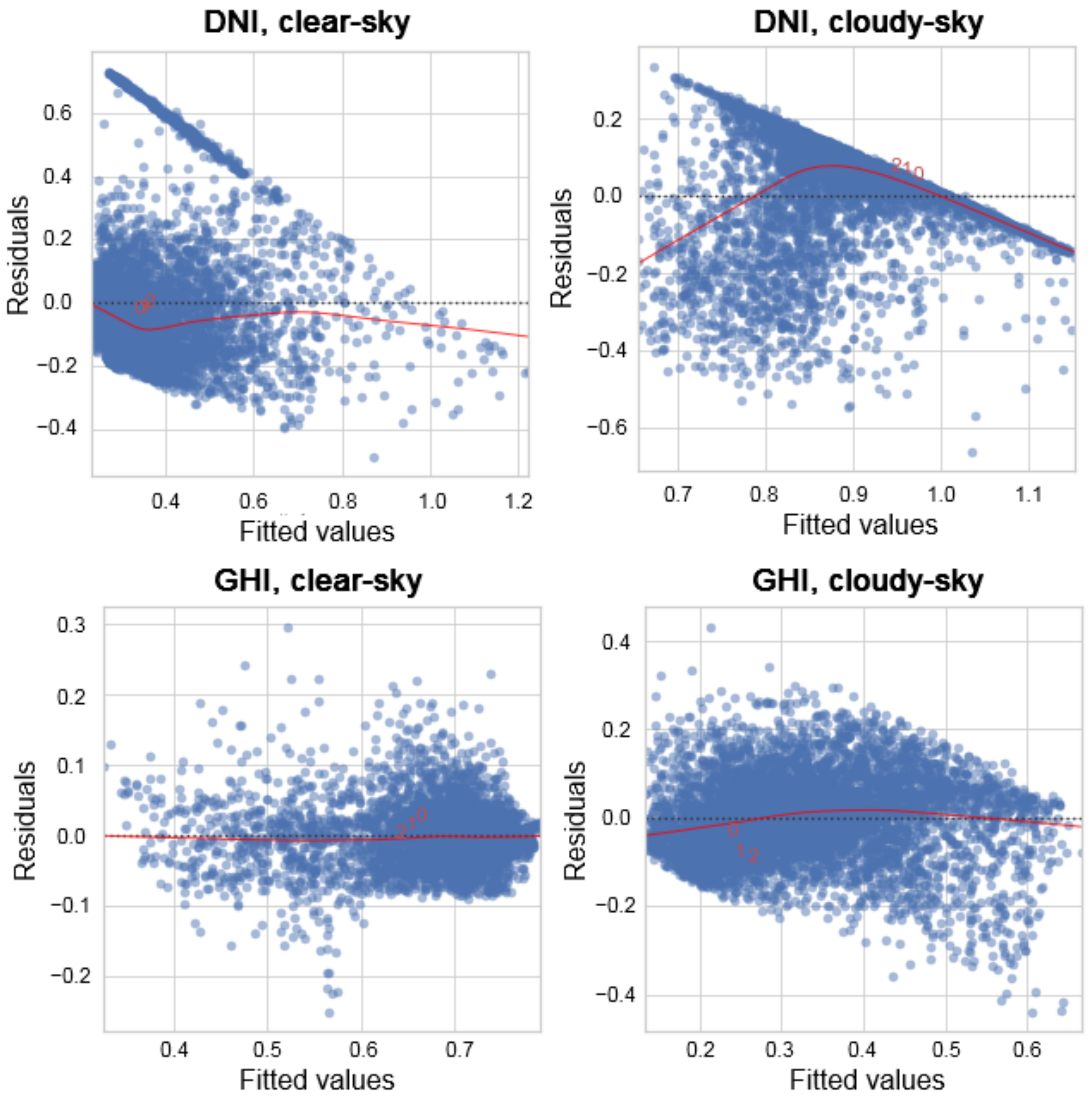
In addition, residual plots (Figure 10) were produced to visually check the nonlinearity of data, from which we can derive what has not yet been accounted for in our model. In the case of GHI, the residual plots exhibited a relatively normal distribution with linearity, as indicated by the roughly horizontal red line. However, in the case of DNI, an abnormal pattern was observed, which may indicate a curvilinear dataset or non-constant variance. Correction for this case may include transforming the response variable to make the variance constant or fitting a more general model instead of a linear model. Further analysis using partial residual plots is required to determine the appropriate transformation.
Combining the analysis for both GHI and DNI under clear- and cloudy-sky conditions in our results, it can be concluded that it is difficult to determine a single site-adaptation method that will significantly improve the accuracy of the global and direct components of solar irradiance estimates under every sky condition. The best site adaptation method differs for different solar irradiance components and sky conditions, and it has not yet been tested on other datasets with different periods or site locations. Therefore, it is suggested to utilize the same collection of site-adaptation methods as a package, followed by the implementation of a ranking algorithm to select the best-corrected dataset. The workflow presented in this study can be utilized to test the performance of site-adaptation methods for more datasets in different time periods or sites to obtain more general results.

5.2. Ranking of Site-Adaptation Methods

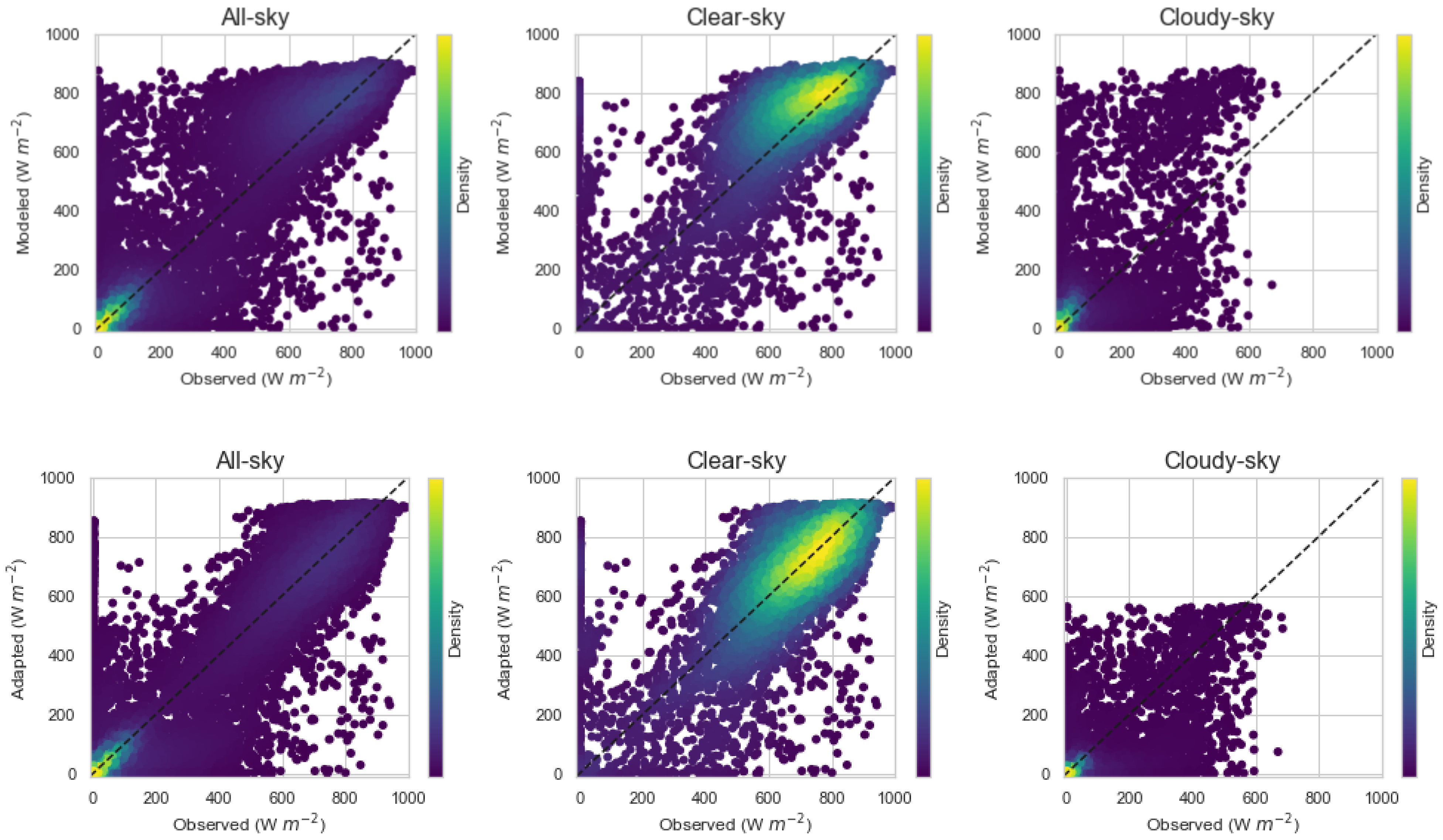
Complete rankings based on each statistical metric value are shown in Table 2 and Tables S1–S5. The best method for each solar irradiance component and sky condition, along with the error metrics is summarized in Table 4. The initial metrics are denoted by “Init.” and metrics after site-adaptation are denoted by “SA”. Moreover, Figure 3 and Figure 4 illustrate the scattered plots of the best site-adapted values for GHI and DNI under each condition, respectively.
It was found that for GHI, sequential methods performed better than individual methods. Under the clear-sky condition, the MLR-Polyfit method exhibited the best performance and it could reduce the MBE, RMSE, and KSI from −3.99% to 0.99%, 12.60% to 5.73%, and 98.67% to 33.04%, respectively. Meanwhile, the MLR-QM some method reduced the MBE, RMSE, and KSI from −6.75% to −2.77%, 36.09% to 30.55%, and 134.33% to 51.27%, respectively, under cloudy-sky conditions.
In contrast, individual methods performed better than sequential methods for DNI site adaptation. Under the cloudy-sky condition, the Polyfit method reduced the MBE, RME, and KSI from 50.59% to −19.88%, 206.80% to 135.36%, and 250.27% to 122.49%, respectively. Under the clear-sky condition, the QDM method exhibited the best performance; however, the reduction in MBE via this method was accompanied by an increase in MABE and RMSE, indicating a change in characteristic from unsymmetrical to symmetrical bias (i.e., the negative and positive bias were in balance), and larger discrepancies were observed at one or more points because the RMSE characteristically puts more weight on the larger error owing to the quadratic factor. As a solution, the second-best ranked method was considered to be the best method for correcting this case, i.e., the Polyfit method, which reduced the MBE, MABE, RMSE, and KSI from 6.67% to 1.27%, 23.67% to 23.65%, 35.99% to 35.11%, and 194.56% to 68.91%, respectively. The overall ranking of the QM many method was the same as that of the Polyfit method, but it yielded worse MABE, RMSE, and OVER. Therefore, the Polyfit method was selected as the best case. This may suggest a requirement to specify a post-ranking evaluation before determining the best technique for future uses.

6. Conclusions

Long-term and reliable solar irradiance data are useful for feasibility studies or site selection in energy projects. For sites where ground observation data are unavailable, solar irradiance can be estimated by satellite-derived models that have large spatiotemporal coverage, but often lack accuracy in comparison to ground observations. The systematic errors in satellite-derived solar irradiance can be corrected by combining short-term ground observation and satellite-modeled data through a process called site-adaptation.
In this study, regressive and distribution mapping site-adaptation methods were performed to correct the global and direct components of solar irradiance (GHI and DNI, respectively) in the UASIBS-KIER model outputs, which is the initial study for South Korea. The GHI and DNI were first separated into clear- and cloudy-sky subsets, and site-adaptation techniques were performed. A sensitivity test of sequential site-adaptation techniques was performed by using the MLR method from regressive families, followed by various distribution mapping techniques. We evaluated the results based on three types of statistical metrics, namely, the error metrics (MBE, MABE, and RMSE), distribution similarity metrics (KSI and OVER), and overall performance (CPI), and produced a ranking based on these values. The results were analyzed for each solar irradiance component and sky condition.
For the GHI, the sequential methods performed better than the individual methods, whereas the opposite was true for DNI. This can be attributed to the intrinsic difference between GHI and DNI or the linear regression problem in the MLR method. For the latter in the case of DNI, it was found that there exist data points with high residuals, low correlation between the response and predictor variables, and the possibility of nonlinear relationships or non-constant variance. Some possible solutions include changing the ordinary least squares method to a robust regression model or a more general model, removing outliers before regression, finding new predictor variables, and transforming the data.
We demonstrated that no site-adaptation method consistently exhibits the best performance for all solar irradiance components. Despite the dominance of the Polyfit method in the case of DNI, the individual metrics and their overall ranking for each method varied. Therefore, the best site-adaptation technique and ranking can be different for different datasets. Accordingly, it may be beneficial to use several site-adaptation techniques in the application of different datasets, as demonstrated in this study, to enable the possibility of maximum site-adaptation correction.
The use of different datasets or producing repeated random sampling by Monte Carlo simulation might be beneficial for evaluating the site-adaptation performance from a probabilistic perspective. Application to different sites may also be beneficial for testing the repeatability and robustness of site-adaptation methods presented here. Moreover, the errors in satellite-derived solar irradiance estimation might be related to difficulties or problems related to cloud condition modeling, which can be a motivation for improving site-adaptation techniques by utilizing cloud parameters such as cloud type, cloud factor, and cloud optical depth. Site-adapted solar irradiance, which is supposed to demonstrate minimized systematic errors, can be further evaluated for application in solar energy simulations. The corrected solar irradiance data through site adaptation may improve the accuracy of solar power generation prediction. Therefore, the calculation of energy production using site-adapted solar irradiance data will be performed in a future study.

Supplementary Materials

The following supporting information can be downloaded at: https://www.mdpi.com/article/10.3390/en15239010/s1. Figure S1: Partial regression plot under cloudy-sky condition for (a) GHI and (b) DNI; Table S1: Statistical metrics and ranking for estimated GHI in clear-sky condition. The rank is provided for each metric (r1-6) and overall rank; Table S2: Same as Table S1 but for estimated GHI in cloudy-sky condition; Table S3: Same as Table S1 but for estimated DNI in all-sky condition; Table S4: Same as Table S1 but for estimated DNI in clear-sky condition; Table S5: Same as Table S1 but for estimated DNI in cloudy-sky condition.

Author Contributions

Conceptualization, C.K.K.; methodology, C.K.K. and E.F.D.; data curation, B.K. and M.O.; software, investigation, visualization, and writing—original draft preparation, E.F.D.; writing—review and editing, C.K.K.; supervision, project administration, and funding acquisition, H.-G.K. All authors have read and agreed to the published version of the manuscript.

Funding

This study was conducted under the framework of the research and development program of the Korea Institute of Energy Research (C2-2410).

Data Availability Statement

The data presented in this study are available on request from the corresponding author.

Acknowledgments

The authors express deep thanks to Chang-Yeol Yun and Jin-Young Kim for their helpful discussions.

Conflicts of Interest

The authors declare no conflict of interest.

References

  1. Choi, Y.; Suh, J.; Kim, S.-M. GIS-Based Solar Radiation Mapping, Site Evaluation, and Potential Assessment: A Review. Appl. Sci. 2019, 9, 1960. [Google Scholar] [CrossRef] [Green Version]
  2. Izadyar, N.; Ong, H.C.; Chong, W.T.; Leong, K.Y. Resource Assessment of the Renewable Energy Potential for a Remote Area: A Review. Renew. Sustain. Energy Rev. 2016, 62, 908–923. [Google Scholar] [CrossRef]
  3. Kim, S.-M.; Oh, M.; Park, H.-D. Analysis and Prioritization of the Floating Photovoltaic System Potential for Reservoirs in Korea. Appl. Sci. 2019, 9, 395. [Google Scholar] [CrossRef] [Green Version]
  4. Yang, D.; Wang, W.; Xia, X. A Concise Overview on Solar Resource Assessment and Forecasting. Adv. Atmos. Sci. 2022, 39, 1239–1251. [Google Scholar] [CrossRef]
  5. Nematollahi, O.; Kim, K.C. A Feasibility Study of Solar Energy in South Korea. Renew. Sustain. Energy Rev. 2017, 77, 566–579. [Google Scholar] [CrossRef]
  6. Kim, C.K.; Kim, H.-G.; Kang, Y.-H.; Yun, C.-Y.; Kim, B.; Kim, J.Y. Solar Resource Potentials and Annual Capacity Factor Based on the Korean Solar Irradiance Datasets Derived by the Satellite Imagery from 1996 to 2019. Remote Sens. 2021, 13, 3422. [Google Scholar] [CrossRef]
  7. Koo, Y.; Oh, M.; Kim, S.-M.; Park, H.-D. Estimation and Mapping of Solar Irradiance for Korea by Using COMS MI Satellite Images and an Artificial Neural Network Model. Energies 2020, 13, 301. [Google Scholar] [CrossRef] [Green Version]
  8. Kim, J.-Y.; Yun, C.-Y.; Kim, C.K.; Kang, Y.-H.; Kim, H.-G.; Lee, S.-N.; Kim, S.-Y. Evaluation of WRF Model-Derived Direct Irradiance for Solar Thermal Resource Assessment over South Korea. AIP Conf. Proc. 2017, 1850, 140013. [Google Scholar] [CrossRef] [Green Version]
  9. Huang, G.; Li, Z.; Li, X.; Liang, S.; Yang, K.; Wang, D.; Zhang, Y. Estimating Surface Solar Irradiance from Satellites: Past, Present, and Future Perspectives. Remote Sens. Environ. 2019, 233, 111371. [Google Scholar] [CrossRef]
  10. Kim, C.K.; Holmgren, W.F.; Stovern, M.; Betterton, E.A. Toward Improved Solar Irradiance Forecasts: Derivation of Downwelling Surface Shortwave Radiation in Arizona from Satellite. Pure Appl. Geophys. 2016, 173, 2535–2553. [Google Scholar] [CrossRef]
  11. Kim, C.K.; Kim, H.-G.; Kang, Y.-H.; Yun, C.-Y. Toward Improved Solar Irradiance Forecasts: Comparison of the Global Horizontal Irradiances Derived from the COMS Satellite Imagery over the Korean Peninsula. Pure Appl. Geophys. 2017, 174, 2773–2792. [Google Scholar] [CrossRef]
  12. Amillo, A.; Huld, T.; Müller, R. A New Database of Global and Direct Solar Radiation Using the Eastern Meteosat Satellite, Models and Validation. Remote Sens. 2014, 6, 8165–8189. [Google Scholar] [CrossRef] [Green Version]
  13. Ineichen, P.; Barroso, C.S.; Geiger, B.; Hollmann, R.; Marsouin, A.; Mueller, R. Satellite Application Facilities Irradiance Products: Hourly Time Step Comparison and Validation over Europe. Int. J. Remote Sens. 2009, 30, 5549–5571. [Google Scholar] [CrossRef]
  14. Riihelä, A.; Kallio, V.; Devraj, S.; Sharma, A.; Lindfors, A. Validation of the SARAH-E Satellite-Based Surface Solar Radiation Estimates over India. Remote Sens. 2018, 10, 392. [Google Scholar] [CrossRef] [Green Version]
  15. Polo, J.; Wilbert, S.; Ruiz-Arias, J.A.; Meyer, R.; Gueymard, C.; Súri, M.; Martín, L.; Mieslinger, T.; Blanc, P.; Grant, I.; et al. Preliminary Survey on Site-Adaptation Techniques for Satellite-Derived and Reanalysis Solar Radiation Datasets. Sol. Energy 2016, 132, 25–37. [Google Scholar] [CrossRef]
  16. Yang, D.; Gueymard, C.A. Probabilistic Post-Processing of Gridded Atmospheric Variables and Its Application to Site Adaptation of Shortwave Solar Radiation. Sol. Energy 2021, 225, 427–443. [Google Scholar] [CrossRef]
  17. Polo, J.; Martín, L.; Vindel, J.M. Correcting Satellite Derived DNI with Systematic and Seasonal Deviations: Application to India. Renew. Energy 2015, 80, 238–243. [Google Scholar] [CrossRef]
  18. Bangarigadu, K.; Hookoom, T.; Ramgolam, Y.K.; Kune, N.F. Analysis of Solar Power and Energy Variability through Site Adaptation of Satellite Data with Quality Controlled Measured Solar Radiation Data. J. Sol. Energy Eng. 2020, 143, 031008. [Google Scholar] [CrossRef]
  19. Cannon, A.J.; Sobie, S.R.; Murdock, T.Q. Bias Correction of GCM Precipitation by Quantile Mapping: How Well Do Methods Preserve Changes in Quantiles and Extremes? J. Clim. 2015, 28, 6938–6959. [Google Scholar] [CrossRef]
  20. Mieslinger, T.; Ament, F.; Chhatbar, K.; Meyer, R. A New Method for Fusion of Measured and Model-Derived Solar Radiation Time-Series. Energy Procedia 2014, 48, 1617–1626. [Google Scholar] [CrossRef]
  21. Schumann, K.; Beyer, H.G.; Meyer, R.; Chhatbar, K. Improving Satellite-Derived Solar Resource Analysis with Parallel Ground-Based Measurements. In Proceedings of the ISES Solar World Congress 2011, Kassel, Germany, 28 August–2 September 2011; pp. 3970–3981. [Google Scholar]
  22. Polo, J.; Fernández-Peruchena, C.; Salamalikis, V.; Mazorra-Aguiar, L.; Turpin, M.; Martín-Pomares, L.; Kazantzidis, A.; Blanc, P.; Remund, J. Benchmarking on Improvement and Site-Adaptation Techniques for Modeled Solar Radiation Datasets. Sol. Energy 2020, 201, 469–479. [Google Scholar] [CrossRef]
  23. Fernández-Peruchena, C.M.; Polo, J.; Martín, L.; Mazorra, L. Site-Adaptation of Modeled Solar Radiation Data: The SiteAdapt Procedure. Remote Sens. 2020, 12, 2127. [Google Scholar] [CrossRef]
  24. McGinnis, S.; Nychka, D.; Mearns, L.O. A New Distribution Mapping Technique for Climate Model Bias Correction. In Machine Learning and Data Mining Approaches to Climate Science; Lakshmanan, V., Gilleland, E., McGovern, A., Tingley, M., Eds.; Springer International Publishing: Cham, Switzerland, 2015; pp. 91–99. ISBN 978-3-319-17219-4. [Google Scholar]
  25. Themeßl, M.J.; Gobiet, A.; Heinrich, G. Empirical-Statistical Downscaling and Error Correction of Regional Climate Models and Its Impact on the Climate Change Signal. Clim. Change 2012, 112, 449–468. [Google Scholar] [CrossRef]
  26. Ramgolam, Y.K.; Bangarigadu, K.; Hookoom, T. A Robust Methodology for Assessing the Effectiveness of Site Adaptation Techniques for Calibration of Solar Radiation Data. J. Sol. Energy Eng. 2020, 143, 31009. [Google Scholar] [CrossRef]
  27. Gueymard, C.A. Clear-Sky Irradiance Predictions for Solar Resource Mapping and Large-Scale Applications: Improved Validation Methodology and Detailed Performance Analysis of 18 Broadband Radiative Models. Sol. Energy 2012, 86, 2145–2169. [Google Scholar] [CrossRef]
  28. Kim, C.K.; Kim, H.-G.; Kang, Y.-H.; Yun, C.-Y.; Lee, Y.G. Intercomparison of Satellite-Derived Solar Irradiance from the GEO-KOMSAT-2A and HIMAWARI-8/9 Satellites by the Evaluation with Ground Observations. Remote Sens. 2020, 12, 2149. [Google Scholar] [CrossRef]
  29. Gueymard, C.A.; Ruiz-Arias, J.A. Extensive Worldwide Validation and Climate Sensitivity Analysis of Direct Irradiance Predictions from 1-Min Global Irradiance. Sol. Energy 2016, 128, 1–30. [Google Scholar] [CrossRef]
  30. Cebecauer, T.; Suri, M. Site-Adaptation of Satellite-Based DNI and GHI Time Series: Overview and SolarGIS Approach. AIP Conf. Proc. 2016, 1734, 150002. [Google Scholar] [CrossRef] [Green Version]
  31. Kasten, F.; Young, A.T. Revised Optical Air Mass Tables and Approximation Formula. Appl. Opt. 1989, 28, 4735–4738. [Google Scholar] [CrossRef] [PubMed]
  32. Kasten, F. The Linke Turbidity Factor Based on Improved Values of the Integral Rayleigh Optical Thickness. Sol. Energy 1996, 56, 239–244. [Google Scholar] [CrossRef]
  33. Perez, R.; Ineichen, P.; Seals, R.; Zelenka, A. Making Full Use of the Clearness Index for Parameterizing Hourly Insolation Conditions. Sol. Energy 1990, 45, 111–114. [Google Scholar] [CrossRef] [Green Version]
  34. Yang, D.; Kleissl, J.; Gueymard, C.A.; Pedro, H.T.C.; Coimbra, C.F.M. History and Trends in Solar Irradiance and PV Power Forecasting: A Preliminary Assessment and Review Using Text Mining. Sol. Energy 2018, 168, 60–101. [Google Scholar] [CrossRef]
  35. Espinar, B.; Ramírez, L.; Drews, A.; Beyer, H.G.; Zarzalejo, L.F.; Polo, J.; Martín, L. Analysis of Different Comparison Parameters Applied to Solar Radiation Data from Satellite and German Radiometric Stations. Sol. Energy 2009, 83, 118–125. [Google Scholar] [CrossRef]
  36. Lorenzo, A.T.; Holmgren, W.F.; Cronin, A.D. Irradiance Forecasts Based on an Irradiance Monitoring Network, Cloud Motion, and Spatial Averaging. Sol. Energy 2015, 122, 1158–1169. [Google Scholar] [CrossRef] [Green Version]
  37. Kim, C.K.; Kim, H.-G.; Kang, Y.-H.; Yun, C.-Y.; Lee, S.-N. Evaluation of Global Horizontal Irradiance Derived from CLAVR-x Model and COMS Imagery over the Korean Peninsula. New Renew. Energy 2016, 12, 13–20. [Google Scholar] [CrossRef]
  38. Ogunjobi, K.O.; Kim, Y.J.; He, Z. Influence of the Total Atmospheric Optical Depth and Cloud Cover on Solar Irradiance Components. Atmos. Res. 2004, 70, 209–227. [Google Scholar] [CrossRef]
  39. Frisch, R.; Waugh, F.V. Partial Time Regressions as Compared with Individual Trends. Econometrica 1933, 1, 387–401. [Google Scholar] [CrossRef] [Green Version]
  40. Lovell, M.C. Seasonal Adjustment of Economic Time Series and Multiple Regression Analysis. J. Am. Stat. Assoc. 1963, 58, 993–1010. [Google Scholar] [CrossRef]
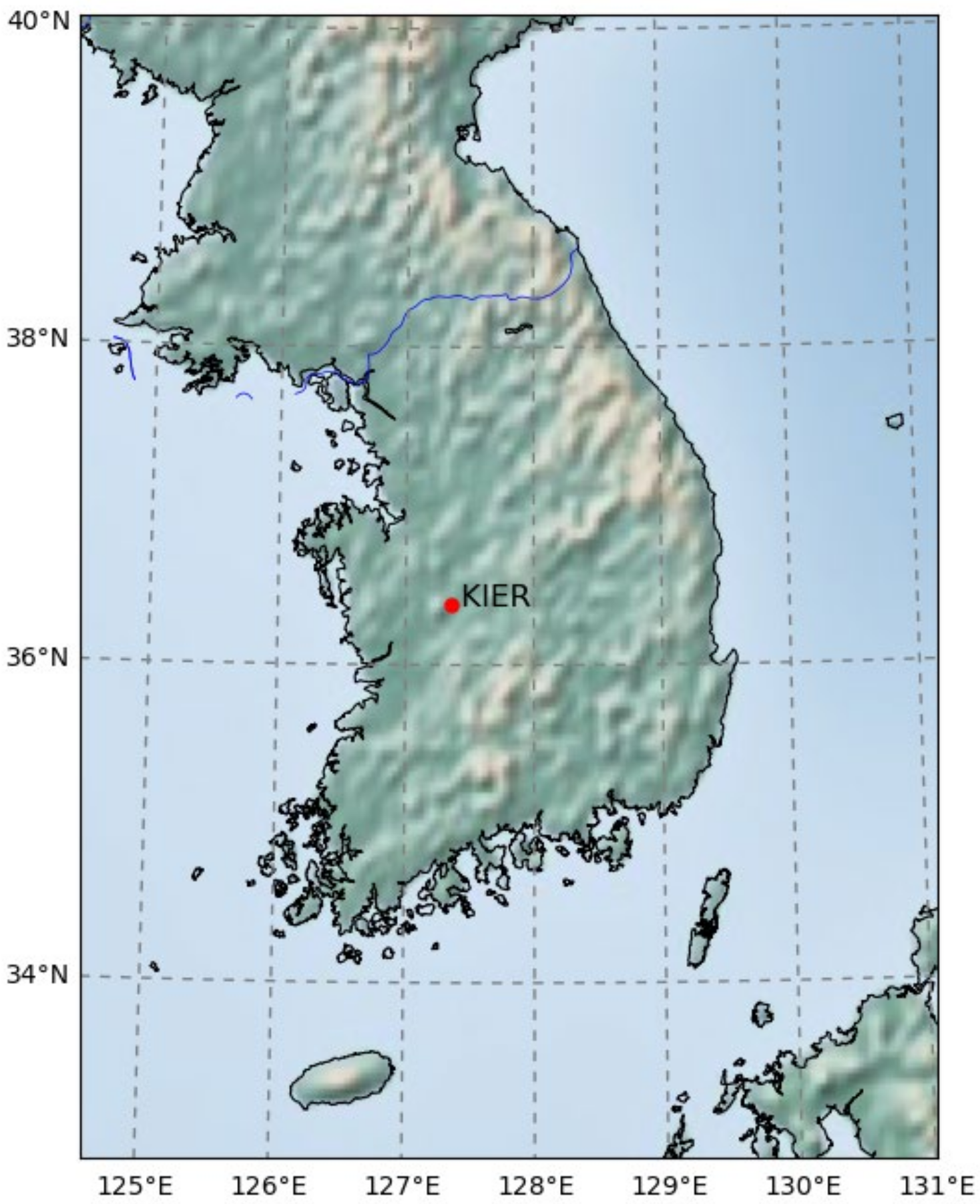
Figure 1. Map of the study site; the red dot indicates the location of ground observation (36.384° N, 127.359° E, 72 m).
Energies 15 09010 g001
Figure 2. Visual representation of regressive (upper panels) and distribution mapping (lower panels) techniques of site-adaptation.
Energies 15 09010 g002
Figure 3. Scatter plots of GHI between satellite estimates and ground observation in the initial state (top) and after site adaptation using the best technique (bottom). The perfect correlation line is indicated by the black dashed line.
Energies 15 09010 g003aEnergies 15 09010 g003b
Figure 4. Same as Figure 3, but for DNI.
Energies 15 09010 g004
Figure 5. Comparison between sequential methods, MLR, and individual distribution mapping techniques for the site adaptation of GHI in clear-sky conditions. The orange bar indicate the best performing sequential method.
Energies 15 09010 g005
Figure 6. Comparison between sequential methods, MLR, and individual distribution mapping techniques for the site adaptation of GHI in cloudy-sky conditions. The orange bar indicate the best performing sequential method.
Energies 15 09010 g006
Figure 7. Same as Figure 5 but for DNI in the clear-sky condition.
Energies 15 09010 g007
Figure 8. Same as Figure 6 but for DNI in the cloudy-sky conditions.
Energies 15 09010 g008
Figure 9. Partial regression plot under clear-sky conditions for (a) GHI and (b) DNI. The plots are scatter plots of residuals from the regression of Y on X ~ i on the y-axis against residuals from the regression of X i on X ~ i on the x-axis. The ordinary least squared fitting line is drawn in black, which indicates the coefficient of X i in the full multiple regression. Figure S1 shows the partial regression plot under cloudy-sky condition.
Energies 15 09010 g009
Figure 10. Residual plots for DNI and GHI cases, which show scatter plots between residuals and the fitted values from MLR. The red smooth curve indicates the fitting of the data.
Energies 15 09010 g010
Table 1. Site-adaptation methods used in this study.
NameFamilyReference
Linear regressionRegressive[18,30]
Polynomial regressionRegressive[20]
Multilinear regressionRegressive[22,23]
Quantile mapping (incl. ECDF Mapping, Kernel Density Estimation (KDE))Distribution mapping[19,24]
Quantile delta mappingDistribution mapping[19]
Polynomial fit of ECDFDistribution mapping[21]
Table 2. Statistical metrics and ranking for estimated GHI in an all-sky condition. The rank is provided for each metric (r1–6) and its overall rank.
MethodMBE (%)r1MABE (%)r2RMSE (%)r3KSI (%)r4OVER (%)r5CPI (%)r6Overall Rank
Initial−5.041814.36921.817136.621763.681760.981717
LIN−3.521715.261721.8918168.931881.871873.651818
POLY−1.091614.691220.29953.4848.96725.7678
MLR−0.671411.18416.461100.291431.31541.131411
ECDF0.37814.671120.791186.821013.581035.51010
QM few1.041515.591821.3916103.711529.011443.871516
QM some0.41914.711320.821286.55912.88835.2789
QM many0.37714.671020.791086.38813.32935.3297
KDE0.22314.741420.831387.381114.711135.931112
QDM0.411015.021621.031596.821324.721340.91315
Polyfit0.18114.761520.941496.071218.871239.211213
MLR-ECDF−0.25411.23616.6654.0161.62422.2155
MLR-QM few0.28612.27817.448109.271633.781644.481614
MLR-QM some−0.21211.28716.64754.371.43322.2566
MLR-QM many−0.25511.23516.59553.5651.64522.143
MLR-KDE−0.451111.15216.47249.2711220.811
MLR-QDM−0.591211.15116.56452.8931.9621.9834
MLR-Polyfit−0.671311.15316.54351.5320.5121.2822
Table 3. Summary of MLR site-adaptation results for GHI and DNI under clear- and cloudy-sky conditions.
GHIDNI
Clear-SkyCloudy-SkyClear-SkyCloudy-Sky
Intercept0.61650.02010.86541.1743
Var10.81001.24950.0430-
Var2−0.4718−0.4536−0.0021−0.0027
Var30.00020.0016−0.5110−0.1718
Var4−0.00600.0310-−0.1975
R-squared0.7830.5800.2710.347
F-statistics41921997575.71025
Table 4. Best ranked method for each solar irradiance component and sky condition.
CaseBest MethodMBE (%)MABE (%)RMSE (%)KSI (%)OVER (%)CPI (%)
Init.SAInit.SAInit.SAInit.SAInit.SAInit.SA
GHI, allMLR-KDE−5.0−0.414.411.121.816.47136.649.363.7161.020.8
GHI, clearMLR-Polyfit−4.01.07.04.312.65.7398.733.0523.842.2536.911.7
GHI, cloudyMLR-QM some−6.7−2.826.522.236.130.55134.451.2756.264.365.729.2
DNI, allPolyfit13.5−2.037.231.562.852.7292.672.61203.66.7155.546.2
DNI, clearPolyfit6.71.323.723.636.035.1194.668.9125.67.4798.0436.6
DNI, cloudyPolyfit50.6−19.9110.373.9206.8135.4250.3122.5157.160.98205.2113.5
Publisher’s Note: MDPI stays neutral with regard to jurisdictional claims in published maps and institutional affiliations.