Prediction of Remaining Useful Life of Lithium Batteries Based on WOA-VMD and LSTM

Abstract

The remaining useful life (RUL) of a lithium-ion battery is directly related to the safety and reliability of the electric system powered by a lithium-ion battery. Accurate prediction of RUL can ensure timely replacement and maintenance of the batteries of the power supply system, and avoid potential safety hazards in the lithium-ion battery power supply system. In order to solve the problem that the prediction accuracy of the RUL of lithium-ion batteries is reduced due to the local capacity recovery phenomenon in the process of the capacity degradation of lithium-ion batteries, a prediction model based on the combination of the whale optimization algorithm (WOA)-variational mode decomposition (VMD) and short-term memory neural network (LSTM) was proposed. First, WOA was used to optimize the VMD parameters, so that the WOA-VMD could fully decompose the capacity signal of the lithium-ion battery and separate the dual component with global attenuation trend and a series of fluctuating components representing the capacity recovery from the capacity signal of the lithium-ion battery. Then, LSTML was used to predict the dual component and fluctuation components, so that LSTM could avoid the interference of the capacity recovery to the prediction. Finally, the RUL prediction results were obtained by stacking and reconstructing the component prediction results. The experimental results show that WOA-VMD-LSTM can effectively improve the prediction accuracy of the RUL of lithium-ion batteries. The average cycle error was one cycle, the average RMSE was less than 0.69%, and the average MAPE was less than 0.43%.

1. Introduction

Lithium-ion batteries are widely used in new energy electric vehicles, power electronics, aerospace, and other fields. Accurately predicting the RUL of a lithium-ion battery can ensure the timely maintenance and replacement of the lithium-ion battery and avoid safety accidents caused by the lithium-ion battery reaching the end of its life [1,2,3,4]. At present, the lithium-ion battery RUL prediction is mainly divided into methods based on physical-mathematical models and data-driven models [5,6]. Data-driven methods can be subdivided into methods based on shallow models and methods based on deep learning models.

The predictive methods based on the physical-mathematical model establish dynamic models by exploring the physicochemical reactions and internal structure of the batteries and achieve RUL prediction by selecting model parameters by using filtering algorithms such as particle filtering [7,8,9] and untraced Kalman filtering [10,11,12]. However, the internal reaction mechanism of the batteries is too complex, and it is difficult to establish an accurate degradation model.

The data-driven prognostics depend on the historical data model and mine the degradation information via various data analysis methods [12,13]. Data-driven methods based on shallow models usually use support vector regression (SVR) [14,15], support vector machines (SVM) [16], extreme learning machine (ELM) [17], related vector machine (RVM) [18,19], Gaussian process regression (GPR) [2,6], and so on. Fang et al. [20] extracted battery health factors, established the relationship between health factors and battery capacity using RVM, and built a health factor prediction model based on ELM. Particle swarm optimization (PSO) has been used to optimize the parameters of RVM and ELM models. Finally, the prediction results of health indicators are added to the RVM model. The experimental results showed that the PSO-ELM-RVM model could effectively predict the RUL of lithium-ion batteries. Yan et al. [21] proposed artificial bee colony (ABC) and genetic algorithm (GA) to optimize the prediction method of SVR core parameters, respectively, to achieve RUL prediction. Patil et al. [16] established a RUL classification and regression model based on key features by using SVM. The classification model provides a rough estimation. If the battery is close to the end of its life, SVR is used to predict RUL. Through key feature extraction and multi-level methods, RUL prediction is not only realized, but the prediction time is also reduced. Pang et al. [2] proposed a new method for the RUL prediction of lithium-ion batteries by integrating incremental capacity analysis (ICA) and GPR. The peak value of the IC curve and the area under the peak value of the IC curve were extracted as health factors, and a RUL prediction model of lithium-ion batteries based on ICA and GPR was established, which realized the RUL prediction of lithium-ion batteries. However, the prediction method proposed in the above literature still has the problem of a low RUL prediction accuracy of lithium-ion batteries.

In recent years, due to the better learning ability of deep learning models in complex system modeling, data-driven methods based on deep learning models have become a hot research field in battery health management. Zhou et al. [22] used empirical mode decomposition to process the capacity attenuation signal of lithium-ion batteries. Subsequently, LSTM was used as the prediction model. The experimental results showed that EMD effectively removed the noise signal and improved the prediction accuracy. Li et al. [23] used EMD to decompose the battery capacity signal into two components: low frequency and high frequency. Elman and LSTM are used to predict low-frequency components and high components, respectively, and the prediction results were reconstructed to obtain the RUL prediction results. However, EMD decomposition is prone to mode aliasing and end-point effects. Chen et al. [24] adopted ensemble empirical mode decomposition (EEMD) to preprocess the collected health factors to reduce the impact of capacity regeneration and noise. Then, phase space reconstruction (PSR) was introduced to realize the selection of the optimal input components, and a genetic algorithm (GA) was used to determine the SVR super parameters to achieve RUL prediction, however, the signal processed by EEMD had residual white noise, and the noise after reconstruction could not be ignored, which affects the accuracy of RUL prediction. Li et al. [25] used complementary ensemble empirical mode decomposition (CEEMD) to decompose the original capacity data into two local fluctuation components with different time scales and one component with long-term memory characteristics. Then, GPR was used to predict two local fluctuation components, and LSTM was used to predict the long-term memory feature components. Finally, the GPR and LSTM prediction results were accumulated and reconstructed to achieve the RUL prediction. However, the disadvantage of CEEMD is that there are differences in the number of components generated during EMD decomposition, which makes it difficult to align components when the final set is averaged or leads to errors in the set average. Lyu et al. [26] obtained trend signals and capacity regeneration signals from the capacity degradation sequence by the VMD algorithm. Then, the trend signal and the capacity regeneration signal were predicted using the particle filter model and the autoregressive integral sliding average model, respectively, and the prediction results of the two signals were superimposed on the capacity degradation prediction. Finally, RUL predictions were made based on the degradation prediction results and failure thresholds. However, because VMD does not sufficiently decompose the degradation signal of the lithium battery capacity, the prediction accuracy is reduced.

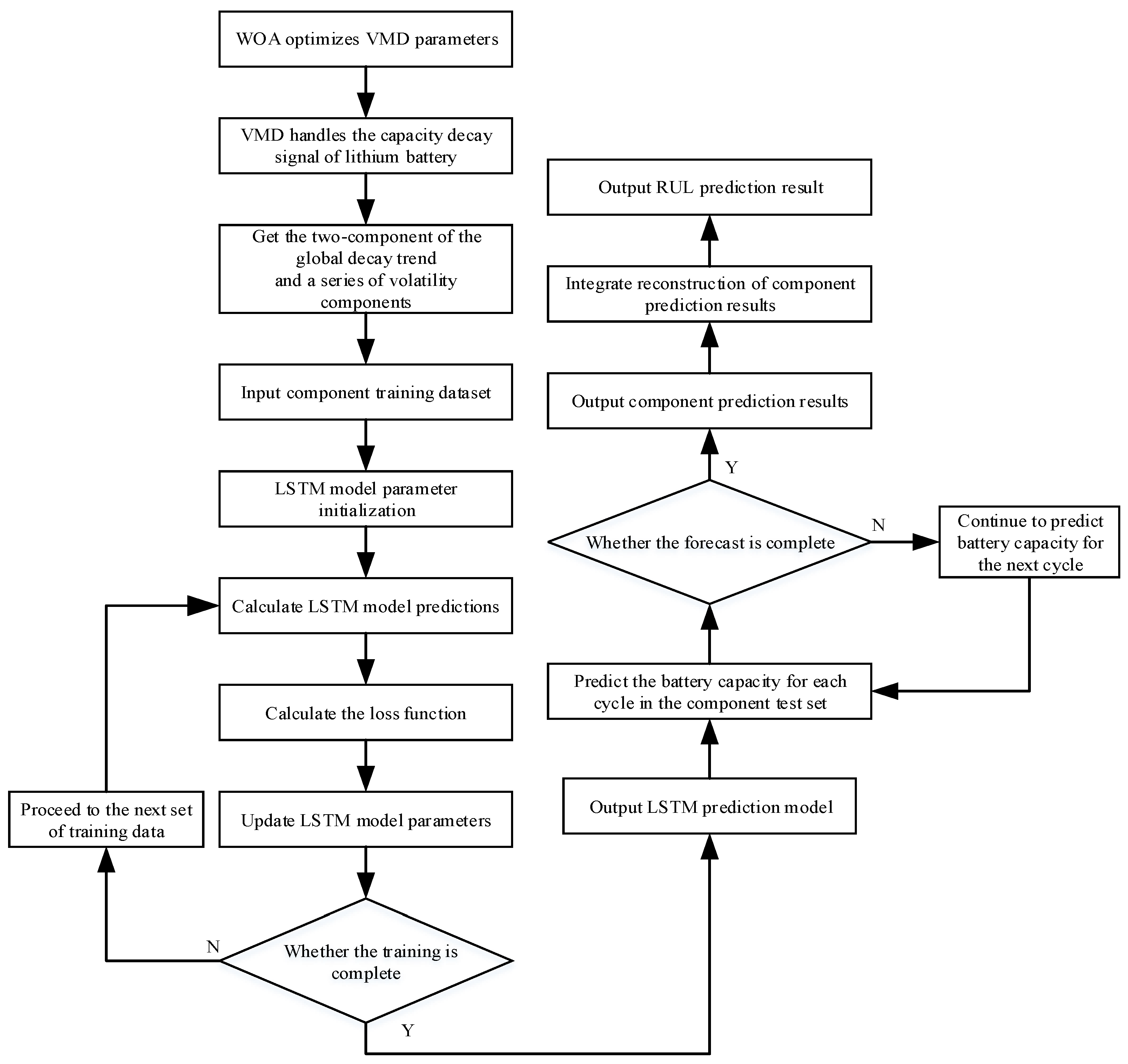
Based on the above analysis, the prediction model composed of the signal decomposition algorithm and deep learning model has obvious advantages in prediction performance, and selecting the appropriate signal decomposition algorithm and deep learning model can effectively improve the prediction accuracy of the RUL. Because VMD can effectively avoid mode aliasing, the endpoint effect, and other problems and has good anti-noise ability and high decomposition efficiency, this paper selected VMD to process the capacity attenuation signal of the lithium battery considering that the parameter modal component K and penalty factor α of VMD affect the decomposition effect of the lithium battery capacity decay signal [27]. 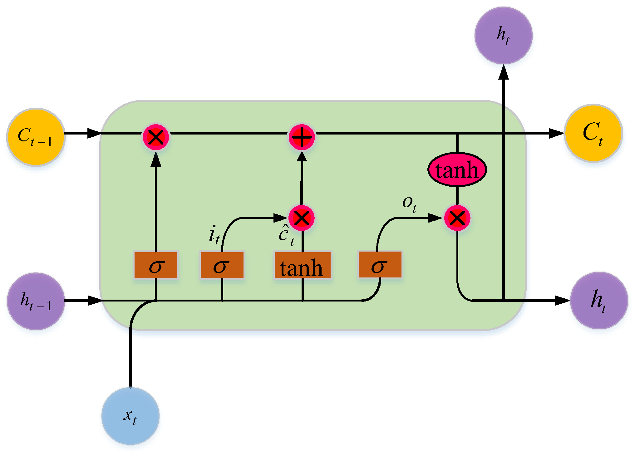The whale optimization algorithm (WOA) with a simple mechanism, few parameters, and strong optimization ability was used to optimize the VMD parameters [28]. Therefore, WOA-VMD can separate the dual component representing the global attenuation trend and a series of fluctuation components representing the capacity recovery from the lithium-ion battery capacity signal, effectively reducing the reconstruction error of the capacity signal. The adopted LSTM can obtain long-term relevant features from the corresponding time series data, which can effectively avoid the problems of gradient disappearance and gradient explosion in the long-sequence training process [29]. LSTM is used to predict the dual component and fluctuation components decomposed by WOA-VMD, and the component prediction results are superposed and reconstructed to obtain the RUL prediction results of lithium-ion batteries.

In summary, the WOA-VMD-LSTM model proposed in this paper can separate the dual component representing the global attenuation trend and the fluctuation component representing the capacity recovery from the lithium-ion battery capacity signal. In the prediction phase of LSTM, WOA-VMD enables LSTM to effectively avoid the interference of capacity recovery to RUL prediction. The experimental results show that WOA-VMD-LSTM can significantly improve the prediction accuracy of RUL.

2. WOA-VMD Model Establishment

2.1. WOA Algorithm

WOA is a bionic intelligent optimization algorithm inspired by the hunting behavior of humpback whales [30]. The humpback whales’ special way of feeding is known as bubble net predation. WOA simulates the approach of searching for prey and the hunting mechanism of humpback whales, which mainly includes three important stages: hunting for prey, prey with a bubble net, and searching for prey [31]. This special predation method gives the WOA algorithm the advantage of a simple mechanism, a few parameters, and strong optimization ability.

The algorithm execution process is as follows:

(1) Initializing the whale position parameter, the position of the nth whale is:

$$X_n=r\cdot \left(ub-lb\right)+lb$$

(1)

Formula (1): r is a random variable of [0, 1]; the value range of X_n is [lb, ub]; lb is the minimum value of the prey range; and ub is the maximum value of the prey range.

(2) Whales have a 50% chance of choosing to round up their prey or prey with bubble nets. When ∣A∣ < 1, the expression corresponding to the whale’s hunting mechanism is shown in Formula (2):

$$\left\{\begin{array}{l}A=2a\cdot r_1-a\\ C=2\cdot r_2\\ a=2-2\left(T/T_{\max }\right)\\ D=\left|C\cdot X^{*}\left(T\right)-X\left(T\right)\right|\\ X\left(T+1\right)=X^{*}\left(T\right)-A\cdot D\begin{array}{cc}& p<0.5\end{array}\end{array}\right.$$

(2)

Formula (2): $r_1,\begin{array}{c}\end{array}{r}_2,\begin{array}{c}\end{array}p$ are all random numbers in [0, 1]; $T$ is the current number of iterations; $T_{\max }$ is the maximum number of iterations; $D$ is the distance between whales and their prey; $a$ linearly reduces from 2 to 0; $X\left(T\right)$ is the current whale position variable; $X^{*}\left(T\right)$ is the current whale best position variable; A and C are the coefficient variable of coefficients that control the way the whale swims [30]. The expression of the bubble net predation model is shown in Formula (3):

$$\left\{\begin{array}{l}X\left(T+1\right)=D^{\prime }\cdot e^{bl}\cdot \cos \left(2\pi l\right)+X^{*}\left(T\right)\begin{array}{cc}& p\ge 0.5\end{array}\\ D^{\prime }=\left|X^{*}\left(T\right)-X\left(T\right)\right|\end{array}\right.$$

(3)

Formula (3): $D^{\prime }$ simulates the distance between whales and prey; b is a constant defining the shape of the spiral; and l is a random number between (−1, 1) [31].

When ∣A∣ ≥ 1, whales randomly wander and hunt, and the position update is shown in Formula (4), where $X_{rand}$ is the randomly selected whale position variable.

$$\left\{\begin{array}{l}X\left(T+1\right)=X_{rand}-A\cdot D\\ D=\left|C\cdot X_{rand}-X\left(T\right)\right|\end{array}\right.$$

(4)

2.2. Variational Mode Decomposition

VMD is an adaptive, quasi-orthogonal, and completely non-recursive signal processing model. Its central idea is to convert the signal decomposition process into a process of finding the optimal solution to an unconstrained variational problem, and it is often used in the processing of non-stationary signals [32]. The VMD principle is to solve the variational problem. In this algorithm, the intrinsic mode function (IMF) is defined as a bandwidth-limited AM-FM function. The function of the VMD algorithm is to construct and solve the constrained variable. The problem is to decompose the original signal into a specified number of IMF components. The corresponding constrained variational model solves the equation as follows:

$$\left\{\begin{array}{c}\underset{\left\{u_k\right\}\cdot \left\{{\omega }_k\right\}}{\min }\left\{{\displaystyle \sum _{k=1}^k{‖{\partial }_t\left[\left(\delta (t)+\frac{j}{\pi t}\right)*u_k(t)\right]e^{-j\omega t}‖}_2^2}\right\}\\ \mathrm{s}.\mathrm{t}.{\displaystyle \sum _k{u}_k(t)=f}\end{array}\right.$$

(5)

Formula (5): $\left\{u_k\right\}$ and are the set of all modes and corresponding center frequencies, respectively; $\delta (t)$ is the Dirac function; K is the number of modes; f is the original signal; $\left(\delta (t)+\frac{j}{\pi t}\right)*u_k(t)$ is the spectrum of after Hilbert transform; * is the convolution operation, and ${\partial }_t$ is the gradient operation.

To solve Formula (5), the Lagrange multiplication operator λ is introduced to transform the constrained variational problem into an unconstrained variational problem, and the augmented Lagrange expression is obtained as:

$$\begin{array}{l}L\left(\left\{u_k\right\},\left\{{\omega }_k\right\},\lambda \right)=\\ \alpha {{\displaystyle \sum _k‖{\partial }_t\left[\left(\delta \left(t\right)+\frac{j}{\pi t}\right)*u_k\left(t\right)\right]e^{-j{\omega }_{k}t}‖}}_2^2+\\ {‖f\left(t\right)-{\displaystyle \sum _k{u}_k\left(t\right)}‖}_2^2+〈\lambda \left(t\right),f\left(t\right)-{\displaystyle \sum _k{u}_k\left(t\right)}〉\end{array}$$

(6)

Formula (6): α is the penalty factor. The original minimization problem is transformed into a saddle point problem with augmented Lagrangian functions using the alternating direction multiplier method.

The specific process of the VMD algorithm is as follows:

(1) According to Formula (7), initialize ${\widehat{u}}_k^1$, ${\omega }_k^1$, ${\lambda }^1$ and n to 0, and select the appropriate number of modes K and penalty factor α.

(2) Iteratively update ${\widehat{u}}_k^1$, ${\omega }_k^1$, ${\lambda }^1$ according to Formula (7)

$$\left\{\begin{array}{l}{\widehat{\lambda }}^{n+1}\left(\omega \right)\leftarrow \widehat{\lambda }\left(\omega \right)+\tau \left(\widehat{f}\left(\omega \right)-{\displaystyle \sum _k{\widehat{u}}_k^{n+1}\left(\omega \right)}\right)\\ {\widehat{u}}_k^{n+1}=\frac{\widehat{f}\left(\omega \right)-{\displaystyle \sum _{i\ne k}{\widehat{u}}_i\left(\omega \right)+\frac{\widehat{\lambda }\left(\omega \right)}{2}}}{1+2\alpha {\left(\omega -{\omega }_k\right)}^2}\\ {\omega }_k^{n+1}=\frac{{\displaystyle {\int }_0^{\infty }\omega {\left|{\widehat{u}}_k\left(\omega \right)\right|}^2\mathrm{d}\omega }}{{\displaystyle {\int }_0^{\infty }{\left|{\widehat{u}}_k\left(\omega \right)\right|}^2\mathrm{d}\omega }}\end{array}\right.$$

(7)

(3) Judging whether the termination conditions are met:

$${\displaystyle \sum _k{‖{\widehat{u}}_k^{n+1}-{\widehat{u}}_k^n‖}_2^2/{‖{\widehat{u}}_k^n‖}_2^2}<\epsilon$$

(8)

Formula (8): $\epsilon$ is the judgment accuracy ($\epsilon >0$). If not satisfied, return to step (2); if satisfied, output K modal components.

2.3. Using WOA to Optimize VMD Parameters

The parameters of the VMD (the number of modes K and the penalty factor α) are optimized by using the WOA algorithm. The value of K will affect the decomposition of the original signal in the time domain. If the value of K is too large, it will lead to excessive decomposition, resulting in some invalid false components. If the value of K is too small, the decomposition of the original signal will be insufficient [33], while the size of α will affect the changing trend of the component signal in the time domain, so it is necessary to determine the optimal combination [K, α] to achieve sufficient decomposition of the signal by VMD. In this paper, the WOA algorithm was used to optimize the VMD parameters, and the minimum value of the envelope entropy was used as the fitness function. Envelope entropy represents a measure of the dynamic information of the original signal [34]. The higher the entropy value, the less information the component contains. In contrast, the smaller the entropy value, the more feature information [35].

The envelope entropy Y of the lithium battery capacity decay signal l(i) (i = 1, 2, 3···, N) can be expressed by Equation (9), where l(i) is the envelope signal of the K component signals decomposed by VMD after Hilbert demodulation; $\epsilon \left(i\right)$ is the probability distribution sequence obtained by calculating the normalization of l(i); N is the number of sampling points; and the entropy value of the calculated probability distribution sequence is the envelope entropy Y.

$$\left\{\begin{array}{l}Y=-{\displaystyle \sum _{i=1}^N\epsilon \left(i\right)\lg \epsilon \left(i\right)}\\ \epsilon \left(i\right)=\frac{l\left(i\right)}{{\displaystyle \sum _{i=1}^{N}l\left(i\right)}}\end{array}\right.$$

(9)

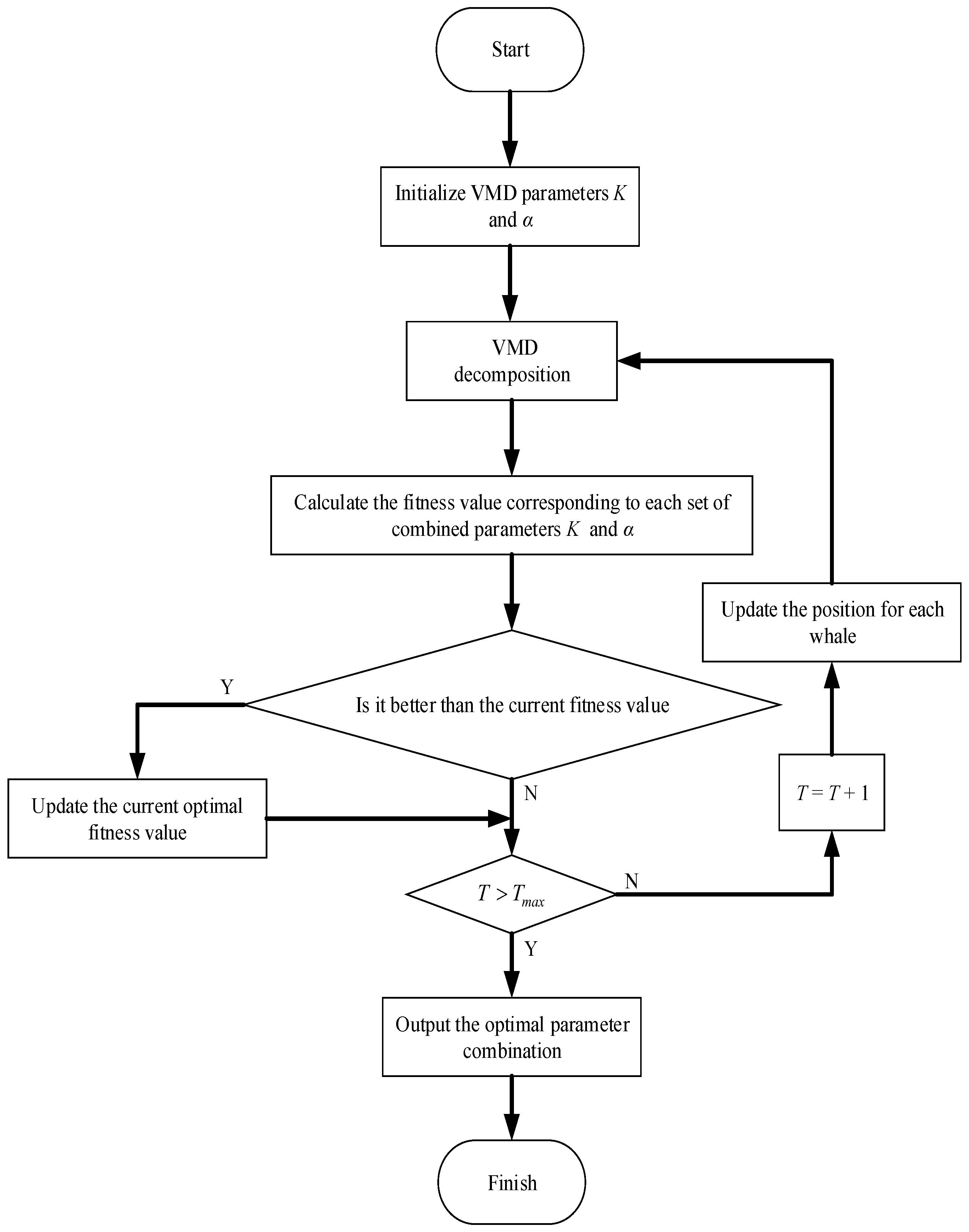
The flowchart of optimizing the VMD parameters using WOA is shown in Figure 1. The specific steps are as follows:

(1) WOA initialization parameters [K, α] set the parameter value range to avoid the range setting being too small, resulting in less feature information in the modal components.

(2) Use VMD to decompose the capacity decay signal of the lithium-ion battery to obtain several IMF components.

(3) Calculate the fitness function value of the corresponding position of each [K, α] and update the best fitness function value when the fitness function value is greater than the current value.

(4) Determine if the iteration is complete. If $T<T_{\max }$, then update the whale’s position variable. Otherwise, the iteration terminates and the optimal parameters [K, α] are saved.

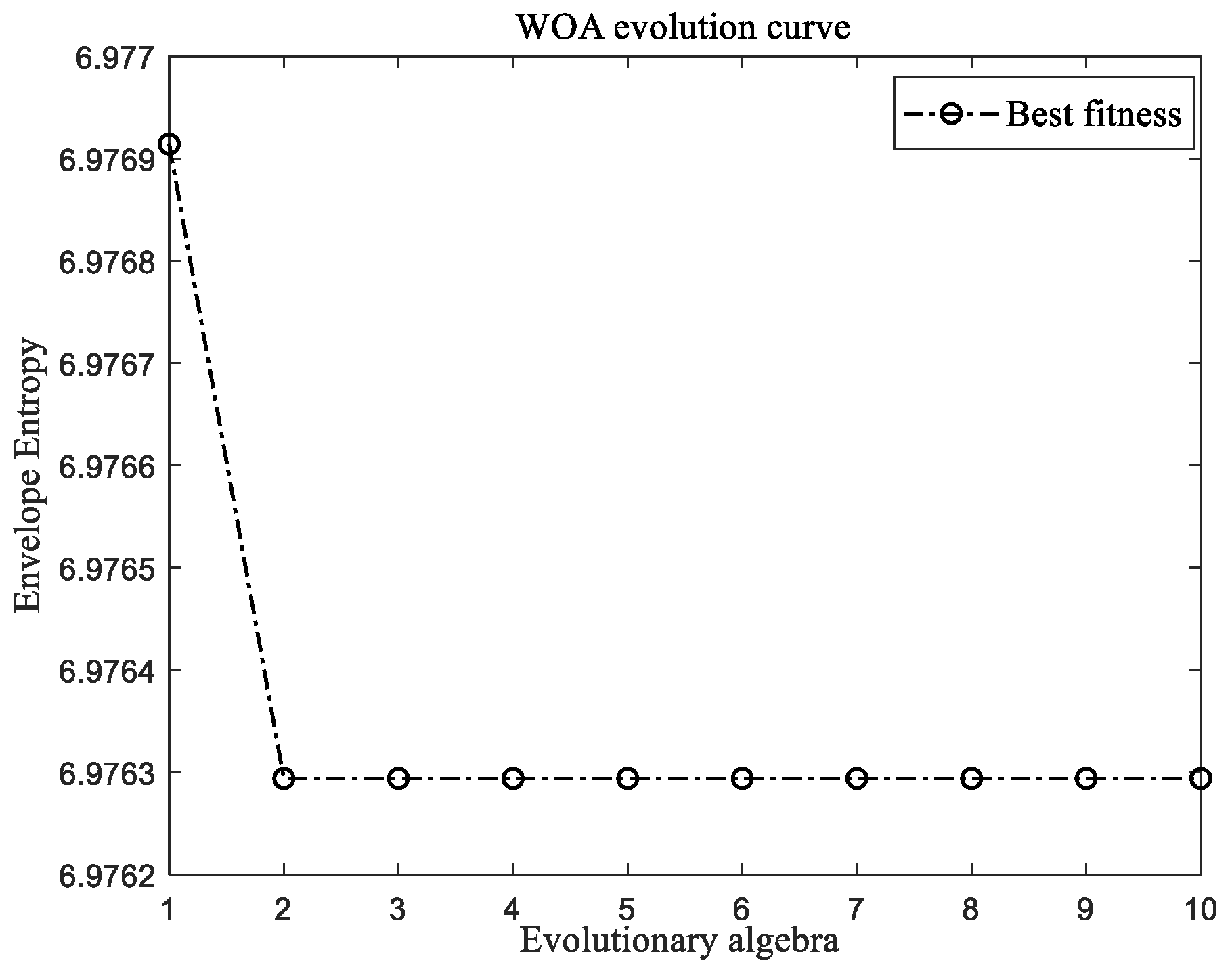
Taking the B5 battery as an example, its fitness changes are shown in Figure 2. It can be seen from Figure 2 that after the WOA evolved twice, the optimal fitness function value was obtained, and the optimization efficiency of the algorithm was obvious.

The optimal parameters of VMD for the B5, B6, B7, and B18 batteries are shown in

Table 1. Optimal parameter of VMD.

Battery	Number of Modes K	Penalty Factor α
B5	6	400
B6	6	480
B7	6	490
B18	5	366

.

3. Predictive Model Building

3.1. Basic Theory of LSTM

The LSTM model can achieve the efficient utilization of long-range information. In addition to some linear interactions, LSTM models add state vectors, and neurons control the stored information through the “gate” structure [36]. The LSTM model has three gates, namely the forget gate, input gate, and output gate [37]. These gates are composed of a sigmoid nonlinear activation function and point multiplication operation. The model structure is shown in Figure 3.

Where $x_{{}^t}$ is the input value of the input layer at this moment and the output value $C_{{}^{t-1}}$ of the hidden layer at the previous moment [38]. The state update steps of the model during training are as follows:

(1) Update the forgetting gate value: $W_f$ is the forgetting gate weight; $b_f$ is the forgetting gate bias; the expression of $f_t$ is shown in Formula (10); $h_{t-1}$ is the data of the hidden layer at moment t − 1:

$$f_t=\sigma \left(W_{xf}{x}_t+W_{hf}{h}_{t-1}+b_f\right)$$

(10)

(2) Linearly transform input $x_t$ at the current moment and input $h_{t-1}$ at the previous moment to obtain a new input ${\widehat{c}}_t$:

$${\widehat{c}}_t=\tanh \left(W_{xc}{x}_t+W_{hc}{h}_{t-1}+b_c\right)$$

(11)

(3) Update the input gate value $i_t$, the input gate controls the current input $x_t$, $i_t$ will store the information of $x_t$ to a limited extent, and the expression of $i_t$ is:

$$i_t=\sigma \left(W_{xi}{x}_t+W_{hi}{h}_{t-1}+b_i\right)$$

(12)

(4) Update the current state vector $c_t$:

$$C_t=f_t{C}_{t-1}+i_t\tanh \left(W_{xc}{x}_t+W_{hc}{h}_{t-1}+b_c\right)$$

(13)

(5) Calculate the output gate, and output the state vector $o_t$ of the hidden layer with limit through the activation function:

$$o_t=\sigma (W_{xo}{x}_t+W_{ho}{h}_{t-1}+b_o)$$

(14)

(6) Memory unit output:

$$h_t=o_t\tanh \left(C_t\right)$$

(15)

Because the existence of “gates” and shared parameters make each neural unit have high stability, it can effectively handle long-distance predictions.

3.2. Prediction Realization Process of LSTM

This paper proposed a lithium-ion battery RUL prediction model based on the combination of WOA-VMD and LSTM. First, the VMD parameters are optimized by WOA, so that the VMD can fully decompose the lithium-ion batteries’ capacity decay signal, and decompose the dual component with the global decay trend, and the fluctuation component representing the local capacity recovery phenomenon from the original signal. The components are divided into a certain proportion of training sets and test sets. After the training stage is completed, the component data are input into the LSTM model in the prediction stage to realize the component prediction, and then the component prediction results are integrated and reconstructed to realize the lithium-ion batteries’ RUL prediction. The overall method flow is shown in Figure 4, and its specific steps are:

(1) Use the WOA algorithm to optimize the VMD parameters [K, α] to obtain the optimal parameters [K, α].

(2) Use VMD under the optimal parameters to fully decompose the lithium-ion batteries’ capacity decay signal, a dual component with a global decay trend, and a series of fluctuation components representing the capacity recovery phenomenon are obtained.

(3) Divide the decomposed components into a certain proportion of training datasets to train the LSTM network, and use the test datasets to test the prediction results.

(4) Finally, the results of the component prediction are integrated and reconstructed to obtain the RUL prediction result.

4. Experimental Verification and Analysis

4.1. Lithium Battery Experimental Data Introduction and Analysis

The experimental data in this paper came from a public dataset provided by NASA PCoE. One set of 18,650 type lithium-ion batteries (B5, B6, B7, B18) were selected for the charge and discharge data collected under the same working conditions, and the rated capacity of the battery was 2 Ah [39]. The standard charging method was adopted, and the maximum cut-off voltage was 4.2 V. Initially, the constant current charging was performed with a current of 1.5 A. When the charging voltage of the battery reached 4.2 V, it switched to constant voltage charging. 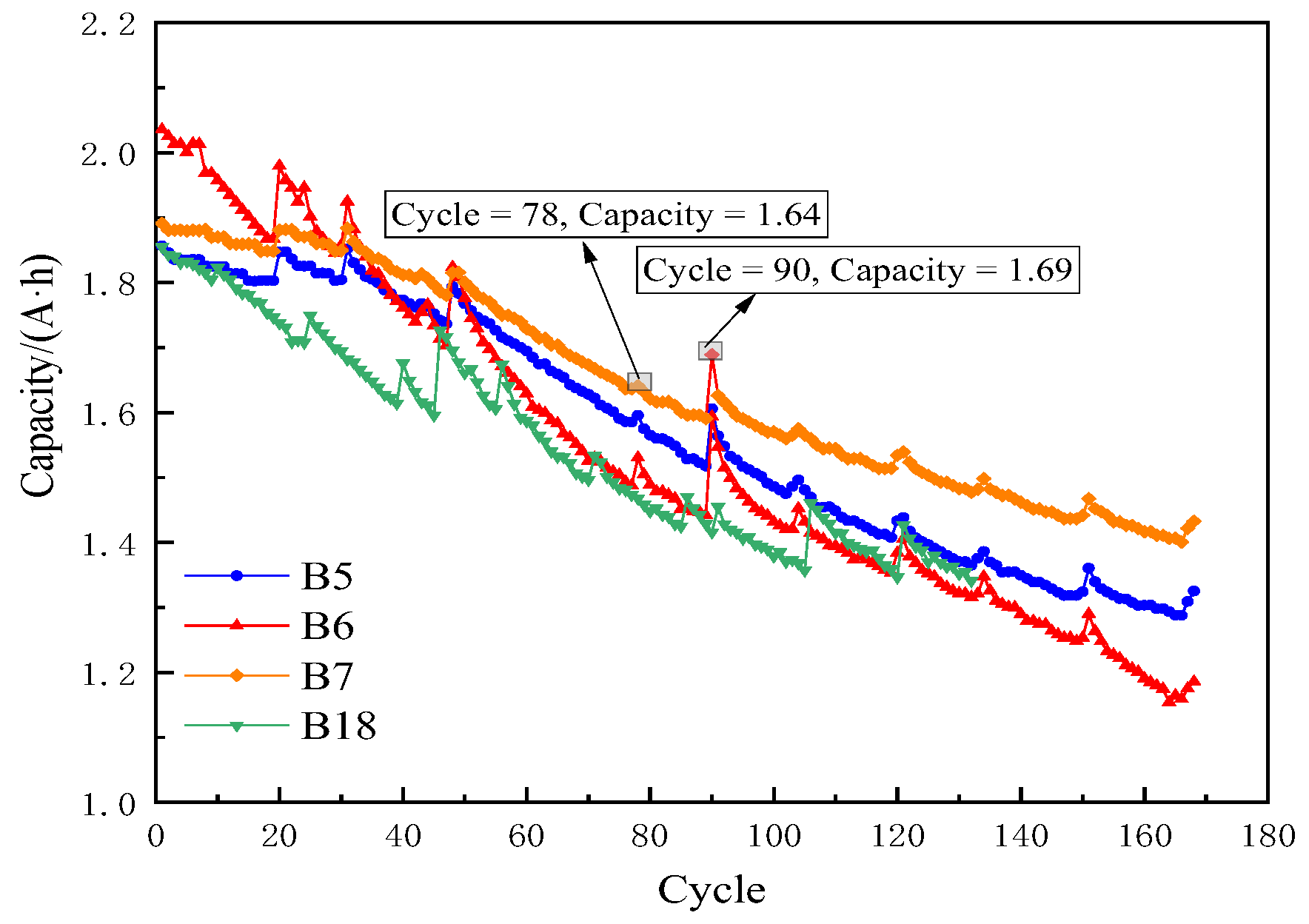When the charging current dropped to 20 mA, the charging ended, and finally discharged with a constant current of 2 A, and took the corresponding capacity changes when the voltages of the B5, B6, B7, and B18 batteries dropped to 2.7 V, 2.5 V, 2.2 V, and 2.5 V, respectively, as the discharge capacity of each cycle [40]. The capacity decay curve of the lithium-ion batteries is shown in Figure 5. It can be seen from Figure 5 that with the increase in the lithium-ion battery cycle period, the overall change in the capacity continues to decrease, but there was a phenomenon of capacity increase in a local area, which is the phenomenon of capacity recovery. In Figure 5, part of the capacity recovery phenomenon is marked. It is generally believed that when the capacity decays to 70% of the original capacity, the battery life reaches the end of life (end of life, EOL) [41]. Therefore, the failure threshold of the B5, B6 and B18 batteries selected in this paper was 1.4 Ah, however, the capacity of the B7 battery did not decrease to 1.4 Ah, so the failure threshold of the B7 battery was set to 1.45 Ah.

4.2. Definition of RUL and Evaluation Criteria for Forecasting Methods

The difference between the number of cycles when the capacity of the lithium-ion batteries was reduced to the failure threshold and the predicted starting point was defined as the RUL of the battery. Assuming that $T_{START}$ is the starting point of prediction, and $T_{EOL}$ is the cycle period when the battery reaches the failure threshold, the real RUL of the battery can be defined as:

$$T_{RUL}=\left|T_{EOL}-T_{START}\right|$$

(16)

The predicted RUL for the battery is:

$$T_{PRUL}=\left|T_{PEOL}-T_{START}\right|$$

(17)

In Formula (17), $T_{PEOL}$ is the number of cycles experienced when the battery reaches the failure threshold in the predicted case.

The accuracy of the prediction method is measured by four common indicators: absolute error (AE), mean absolute error (MAE), root mean square error (RMSE) and mean absolute percentage error (MAPE).

The formula for calculating the four error indicators is as follows:

$$AE=\left|T_{RUL} - T_{PRUL}\right|$$

(18)

$$MAE=\frac{1}{N}{\displaystyle \sum _{i=1}^N\left|C_R\left(i\right)-C_P\left(i\right)\right|}$$

(19)

$$RMSE=\sqrt{\frac{1}{N}{\displaystyle \sum _{i=1}^N{\left|C_R\left(i\right)-C_P\left(i\right)\right|}^2}}$$

(20)

$$MAPE=\frac{1}{N}{\displaystyle \sum _{i=1}^N\frac{\left|C_R\left(i\right)-C_p\left(i\right)\right|}{C_R\left(i\right)}}\times 100\%$$

(21)

In Formula (19) to Formula (21), $C_R\left(i\right)$ is the true value of the battery capacity, $C_P\left(i\right)$ is the battery capacity prediction, and N is the predicted number of cycles.

4.3. WOA-VMD Analysis and Prediction of Components

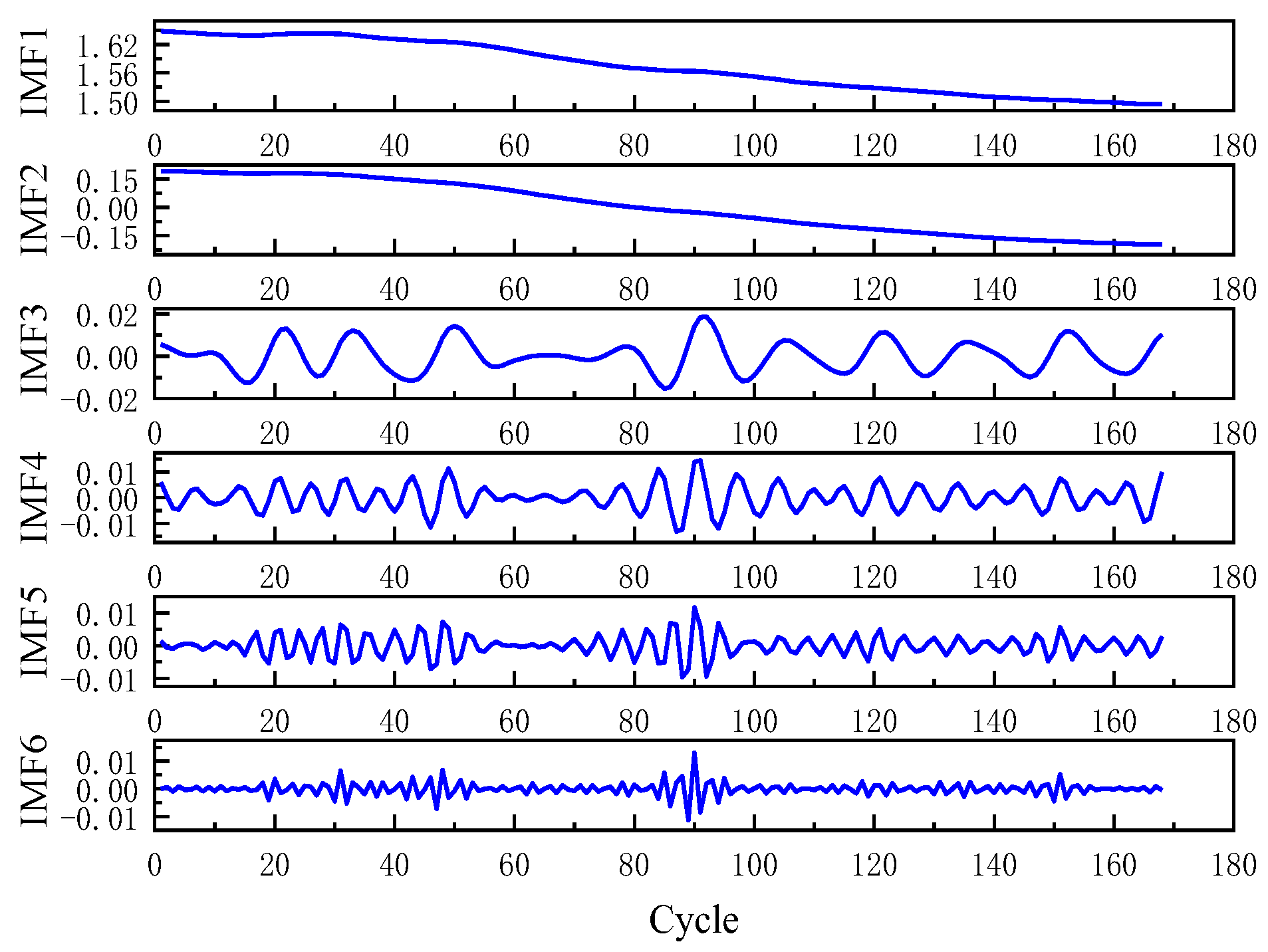
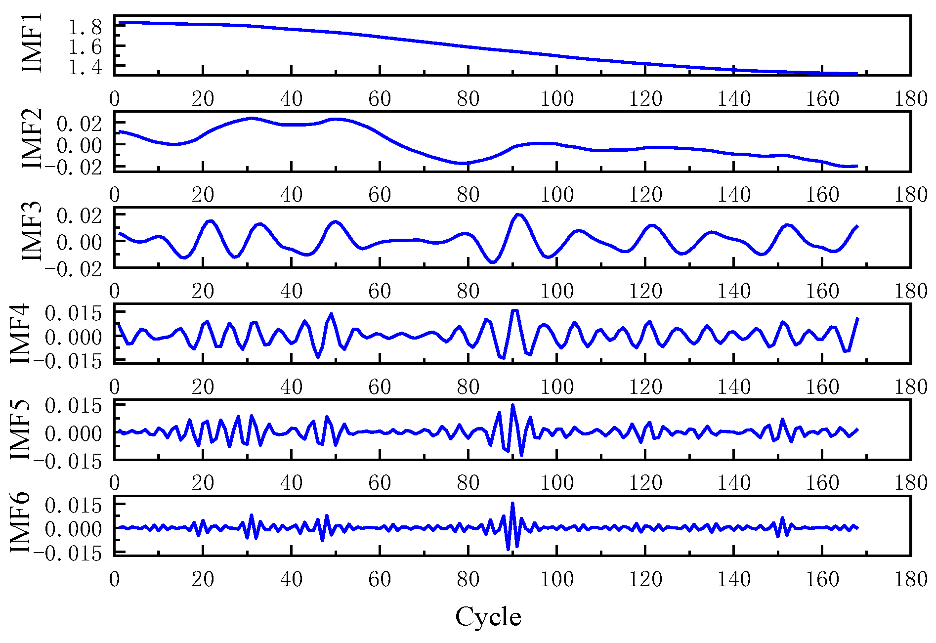
The WOA-VMD was used to decompose the battery capacity decay signal. Taking B5 as an example, the optimized VMD parameters K and α were 6 and 400, respectively, and the decomposed modal components are shown in Figure 6, among them, IMF1 and IMF2 represent the dual components of the lithium battery capacity decay signal with a global decay trend, and the remaining components can be regarded as the fluctuation components that represent the local capacity recovery phenomenon.

To verify the influence of α on the component signal, K was set to 6, and α was set to 800 and 100, respectively, and the decomposition conditions are shown in Figure 7 and Figure 8, respectively.

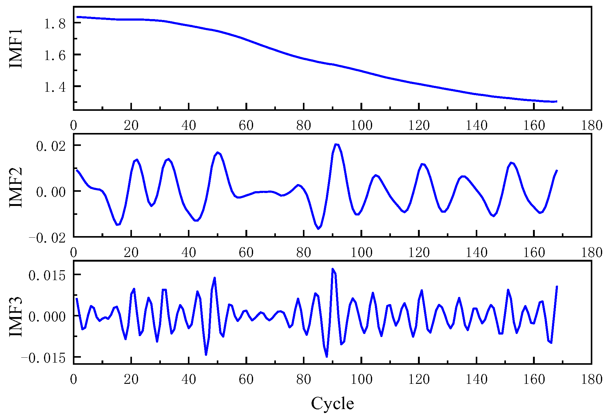
It can be observed from IMF1 and IMF2 in Figure 6, Figure 7 and Figure 8 that when the K values were the same, the size of α will affect the change trend of the component signal. Considering the characteristics of global attenuation, capacity recovery, and random fluctuation in the process of battery degradation, the K value of VMD decomposition was set to 3, and the α value was set to 400 to verify the influence of the K value on the component signals. The decomposition effect is shown in Figure 9.

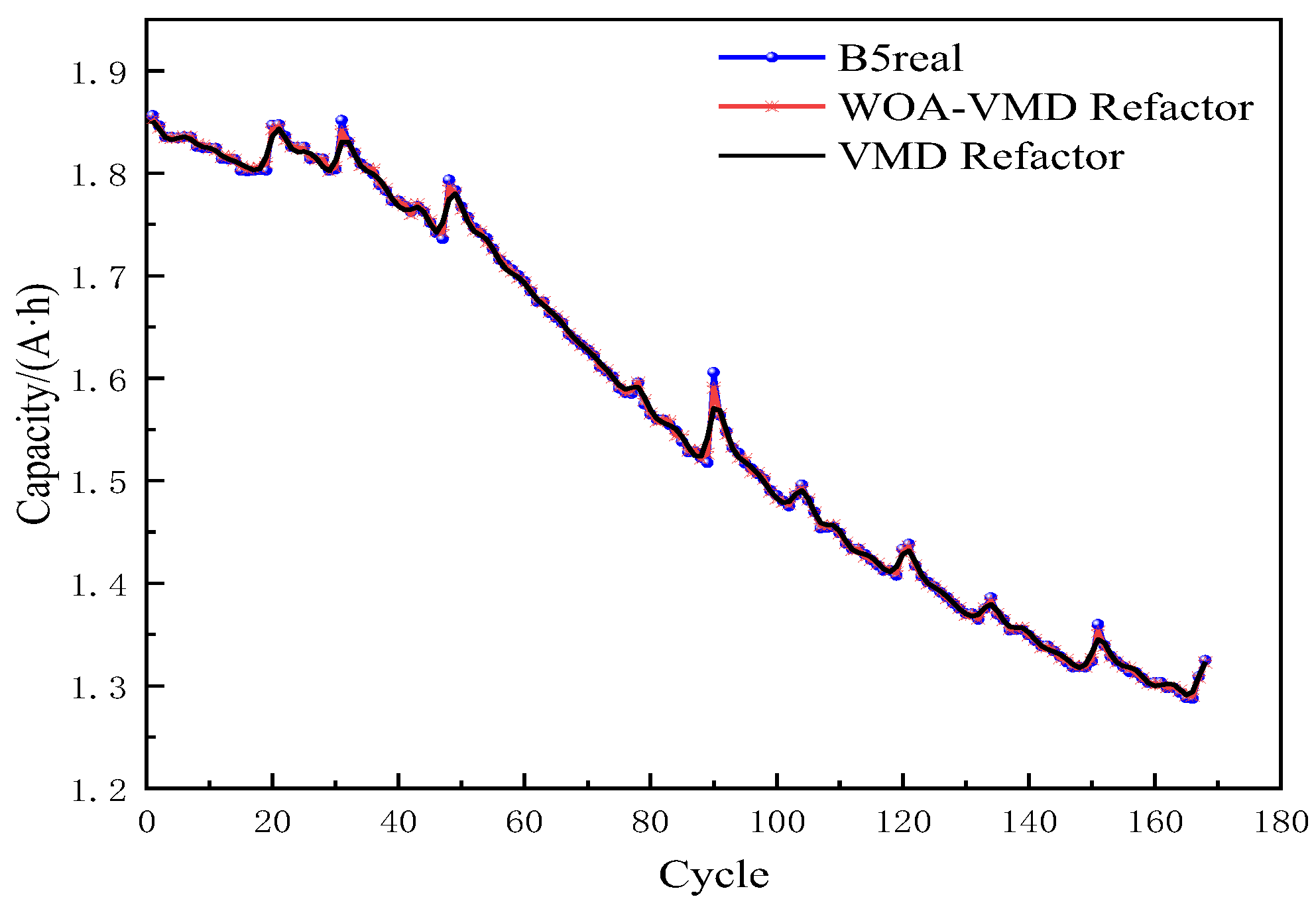
By comparing Figure 6 and Figure 9, it can be seen that when α at the same K = 3, the VMD could only decompose a single IMF1 component with a global decay trend. The WOA-VMD refactoring signal and the VMD refactoring signal are now reconstructed (at this time, the VMD parameter K = 3, α = 400) in contrast to the original signal, as shown in Figure 10. As can be seen from Figure 10, the WOA-VMD reconstructed signal was closer to the original signal, and the WOA-VMD fit better in local areas where capacity rebound occurred.

To further illustrate that WOA-VMD could fully decompose the capacity decay signal of lithium battery, we calculated the Pearson correlation coefficient between the trend component of Figure 6, Figure 7 and Figure 8 and the B5 battery capacity, respectively, and the results are shown in

Table 2. Correlation coefficient between the component signal and capacity.

Figure	IMF	B5
Figure 6	IMF1	0.99806
	IMF2	0.99779
Figure 7	IMF1	0.90298
	IMF2	0.99744
Figure 8	IMF1	0.99686
	IMF2	0.77803
Figure 9	IMF1	0.99775

.

From the magnitude of the correlation coefficient in Table 2, it can be seen that the IMF1 and IMF2 fully decomposed by WOA-VMD had the highest correlation coefficient with the capacity information, which could better express the characteristics of the global decay trend of lithium-ion batteries.

Taking the B5 battery as an example, the first 70 sets of capacity data of the component were used as the training set, and the capacity prediction value after the 70th set was used as the output of the LSTM model and compared with the test set; the component prediction results are shown in Figure 11. It can be seen from Figure 11 that the LSTM model maintained a high degree of fitting in each component prediction.

From the above analysis, it can be seen that the two most significant features of a lithium-ion battery are that the capacity signal has the characteristics of a global attenuation trend and local capacity recovery. How to fully extract the characteristics of the global attenuation trend is the key to improving the prediction accuracy of RUL. First of all, WOA-VMD is used to fully decompose the capacity signal of lithium-ion batteries to obtain the dual component with a global attenuation trend. Compared with a single component, the correlation coefficient between the dual component and capacity signal is higher, which can better express the characteristics of the global attenuation trend of a lithium-ion battery; in addition, the error of the WOA-VMD component signal when reconstituting the original signal was smaller.

4.4. Comparison and Analysis of Forecast Results

To verify the superiority of the method in this paper, four comparison methods were designed, as shown in

Table 3. Description of the methods.

Method	Describe
M1	WOA-VMD-LSTM
M2	LSTM
M3	EMD-LSTM
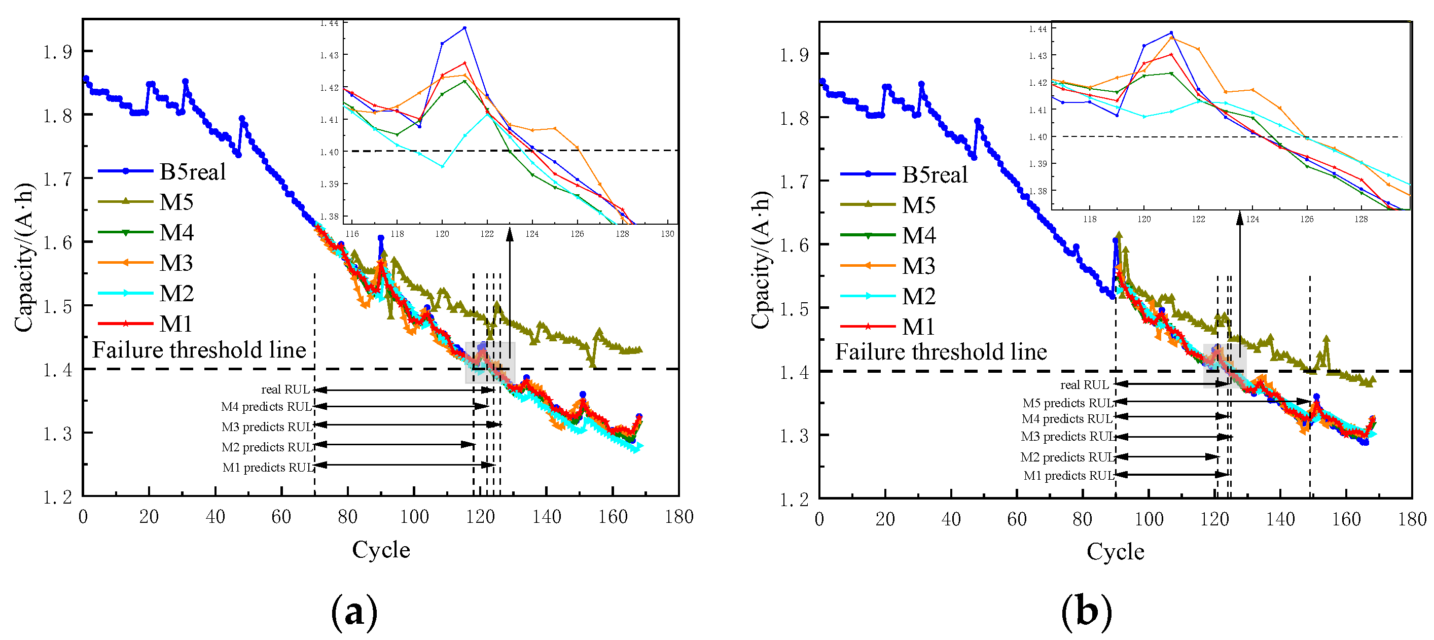
M4	VMD-LSTM
M5	ELM

, and different prediction starting points were set to verify the stability of the method. The prediction starting points of B5, B6, and B7 were 70 and 90. The number of B18 battery data samples was small, and the prediction starting points were set to 55 and 70.

M1 is the method proposed in this paper, M2 is a single LSTM prediction method, M3 is a combination of EMD-LSTM, M4 is VMD-LSTM (parameter K = 3 of VMD, α = 400), and M5 is the ELM prediction method. The superiority of LSTM in the time-series data was highlighted by comparing M2 with M5. By comparing M3, M4, and M2, the combined prediction model significantly improved the prediction accuracy. The combination prediction model of VMD decomposition and LSTM under optimal parameters can further improve the prediction accuracy by comparing M1 with M3 and M4.

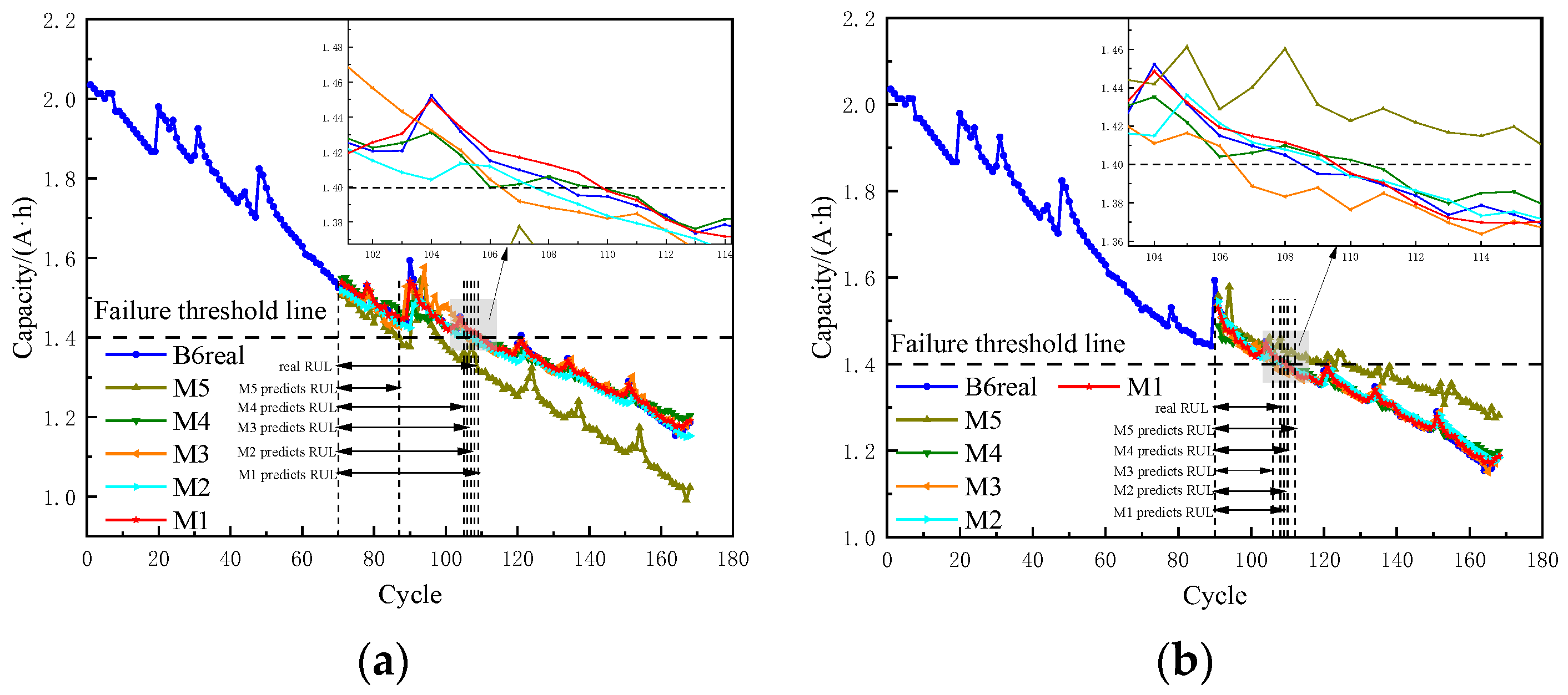
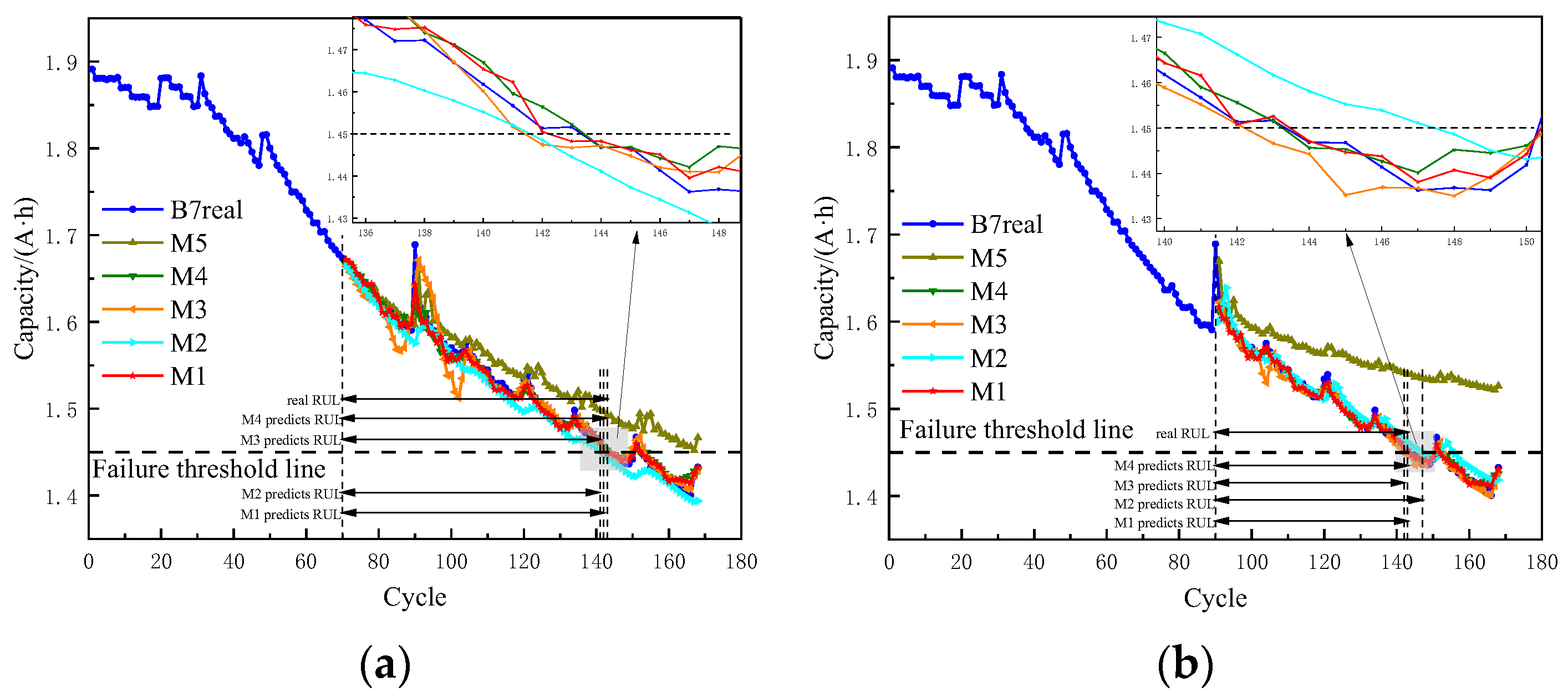
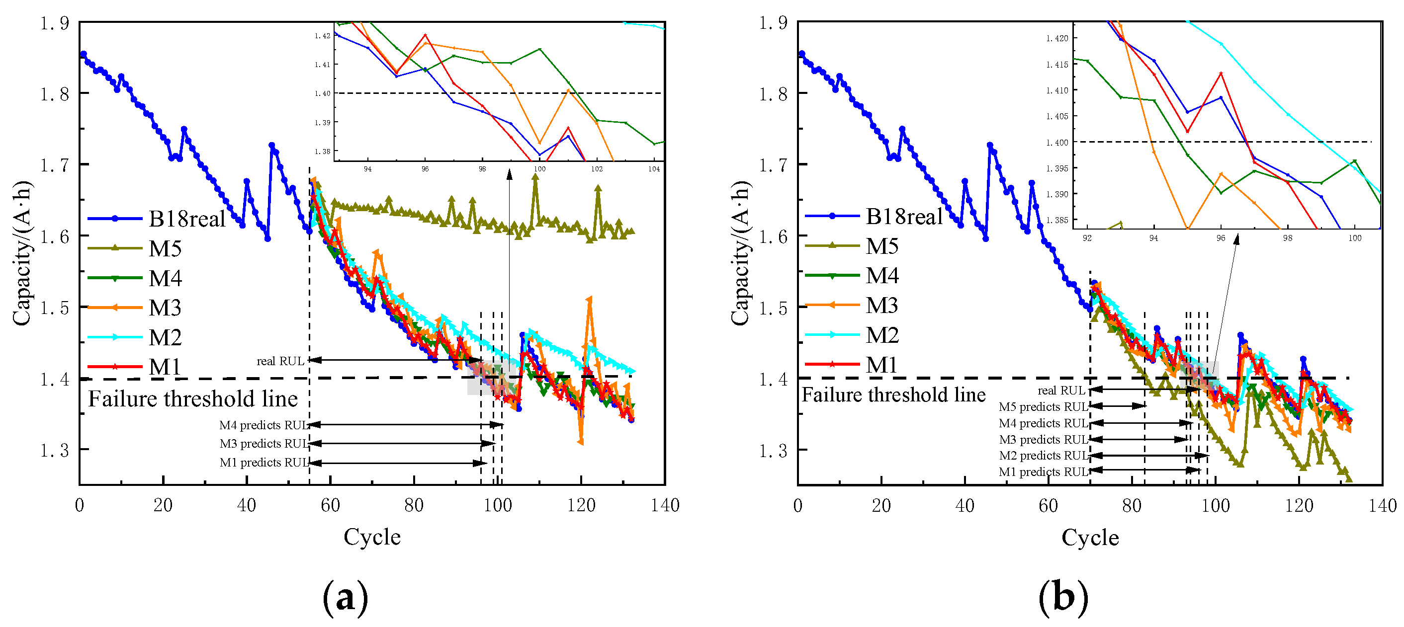
Figure 12, Figure 13, Figure 14 and Figure 15 show the prediction results of B5, B6, B7, and B18 at different starting points. Since the B7 battery did not reach the failure threshold of 1.4 A·h, the failure threshold of the B7 battery was set to 1.45 A·h. Part of the prediction curves of M2 and M5 did not reach the failure threshold, and the AE value could not be calculated, so the corresponding part of Table 3 is represented by ‘−’.

A comparison of the evaluation indicators under different methods is shown in

Table 4. A comparison of the evaluation indicators.

Battery	Start	Method	AE	MAE (%)	RMSE (%)	MAPE (%)
B5	70	M1	0	0.53	0.74	0.37
		M2	6	1.03	1.65	0.73
		M3	2	1.04	1.45	0.72
		M4	0	0.69	1.03	0.48
		M5	-	7.04	8.24	5.14
	90	M1	0	0.48	0.58	0.34
		M2	3	0.96	1.21	0.69
		M3	1	0.85	1.08	0.61
		M4	0	0.56	0.74	0.40
		M5	25	6.22	6.68	4.56
B6	70	M1	1	0.68	0.93	0.50
		M2	1	1.28	2.42	0.92
		M3	2	1.49	2.21	1.07
		M4	3	1.53	2.21	1.12
		M5	11	8.86	9.85	6.73
	90	M1	1	0.50	0.66	0.38
		M2	1	1.11	1.44	0.87
		M3	2	0.86	1.11	0.64
		M4	2	1.36	1.83	1.03
		M5	14	6.25	7.18	4.90
B7	70	M1	1	0.52	0.75	0.34
		M2	2	1.19	1.83	0.78
		M3	2	1.07	1.66	0.68
		M4	0	0.64	1.00	0.42
		M5	-	2.70	3.22	1.82
	90	M1	0	0.38	0.47	0.25
		M2	4	1.01	1.23	0.68
		M3	1	0.51	0.80	0.34
		M4	0	0.45	0.61	0.30
		M5	-	6.43	7.18	4.39
B18	55	M1	1	0.85	0.75	0.58
		M2	-	4.02	4.41	2.82
		M3	3	2.19	2.61	1.52
		M4	5	2.10	2.39	1.45
		M5	-	1.71	1.85	12.03
	70	M1	0	0.53	0.72	0.36
		M2	2	1.95	2.39	1.37
		M3	3	1.63	2.14	1.16
		M4	2	1.56	2.23	1.10
		M5	13	5.95	6.82	4.23

.

To further illustrate the superiority of the proposed method, the results of this method were compared with those of the existing literature, as shown in

Table 5. A comparison of the prediction performance with the existing results.

Method	B5		B6		B7		B18
	RMSE	AE	RMSE	AE	RMSE	AE	RMSE	AE
Proposed method	0.0048	0	0.0051	1	0.0036	0	0.0055	0
PSR-GASVR-EC [23]	0.0191	0	0.0081	1	0.0101	1	0.0051	0
ALF-PF-LSTM [6]	0.0116	1	0.0161	2	0.0110	0	-	-
VPA [25]	0.2562	-	0.2367	-	0.6267	-	0.6575	-

. The predicted starting point of the B5, B6, and B7 batteries was 100, and that of the B18 battery was 80. At the same time, the influence of training sets of different sizes on the prediction performance of the model is shown in

Table 6. Comparison of the prediction performance with different amounts of training data.

Start	B5			B6			B7			B18
	RMSE	MAPE	AE	RMSE	MAPE	AE	RMSE	MAPE	AE	RMSE	MAPE	AE
60	0.96%	0.59%	2	1.02%	0.54%	0	0.82%	0.42%	2	0.86%	0.47%	1
70	0.74%	0.37%	0	0.93%	0.50%	1	0.75%	0.34%	1	0.72%	0.36%	0
80	0.64%	0.36%	1	0.81%	0.46%	1	0.68%	0.32%	1	0.51%	0.30%	1
90	0.58%	0.34%	0	0.66%	0.38%	1	0.47%	0.25%	0	-	-	-
100	0.48%	0.30%	0	0.51%	0.30%	1	0.36%	0.19%	0	-	-	-

.

By comparing the predicted results with the evaluation indicators, the results can be summarized as follows.

(1) From Figure 12, Figure 13, Figure 14 and Figure 15 and Table 4, it was shown that the prediction results of the methods presented in this paper were significantly better than those of LSTM, ELM, EMD-LSTM, and VMD-LSTM. The prediction curve of M1 was closer to the original signal in different groups and different starting points, and the prediction effect was stable, even below the failure threshold.

(2) From Table 6, we can see that the prediction accuracy will be different under different prediction starting points. The more backward the starting point, the more training periods there are, and the lower the prediction error. In the prediction of four batteries, the maximum AE of the proposed method was only 2 when there were few training set samples. Under the test of all training sets, the maximum RMSE was 1.02%, the minimum RMSE was 0.36%, and the average RMSE was less than 0.69%. The maximum MAPE was 0.59%, the minimum MAPE was 0.19%, and the average MAPE was less than 0.43%.

(3) It can be seen from Figure 12, Figure 13, Figure 14 and Figure 15 and Table 4 that the deep learning model LSTM had a better prediction effect than the shallow model ELM. Further analysis of the prediction results of M2 and M3 showed that EMD decomposes the capacity signal to avoid the impact of capacity rebound on M2, making M3 better than M2. Comparing M3, M4, and M1, it was found that the method proposed in this paper (M1) avoids the interference of EMD mode aliasing, the VMD super parameter influence, and the capacity rebound phenomenon on prediction, making the prediction effect of M1 significantly improved. At the same time, according to Table 5, the method in this paper had obvious advantages in prediction accuracy.

5. Discussion

The WOA-VMD-LSTM model proposed in this paper can separate the dual component representing the global attenuation trend and the fluctuation component representing the capacity recovery from the lithium-ion battery capacity signal. In the prediction phase of LSTM, WOA-VMD enables LSTM to effectively avoid the interference of capacity recovery to the RUL prediction. The experimental results showed that WOA-VMD-LSTM could significantly improve the prediction accuracy of the RUL. The innovation of this method is that WOA-VMD is used to fully decompose the capacity signal of the lithium-ion battery, and the dual component with a global attenuation trend is obtained. Compared with the single component, the correlation coefficient between the dual component and the capacity signal is higher, which can better express the characteristics of the global attenuation trend of a lithium-ion battery. Moreover, the component signal of WOA-VMD has less error when reconstituting the original signal.

In Table 5, the ALF-PF-LSTM model uses adaptive Levy flight to optimize the PF and LSTM networks. However, when using ALF to optimize PF, the capacity rebound phenomenon and noise of the lithium-ion battery capacity signal are eliminated, which reduces the prediction accuracy. This is because the capacity rebound phenomenon is the most prominent feature information in the lithium-ion battery capacity signal. The advantage of this method is that it reduces the complexity of prediction and can achieve better prediction results without too many training samples, but the prediction accuracy is reduced. The VPA model in Table 5 first uses VMD to decompose the capacity signal, decomposing a component signal of attenuation trend and two component signals representing the capacity regeneration phenomenon, respectively, using PF and Auto Regenerative Integrated Moving Average Model to predict the attenuation trend signal and capacity regeneration signal, and reconstruct the prediction results of each component to obtain the RUL prediction results. The VPA model has some similarities with the method in this paper. First, we both use VMD to decompose the capacity signal, but the WOA-VMD in this paper decomposes the capacity signal more fully, so the method in this paper can achieve a better prediction effect in the subsequent prediction. The main advantage of the VPA model is its better generalization ability. The PF and ARIMA prediction models are respectively used to predict the components of two different trends. However, this paper only used LSTM as a prediction model to predict the components of different trends. The generalization ability of the model is not strong enough, and it may not be applicable to the datasets of lithium-ion batteries of other types. The PSR-GASVR-EC model in Table 5 extracts a health factor that can represent the capacity signal from the historical data of the lithium-ion battery, uses EEMD to decompose the health factor to obtain multiple sequence signals, and PSR to select the best input sequence. Then, genetic algorithm is used to optimize the kernel function of SVR, and the optimal input sequence is used as the input of GA-SVR to obtain the preliminary prediction results. Finally, error compensation is used to stack the preliminary prediction results to obtain the RUL prediction results. Traditional lithium-ion battery capacity value acquisition requires the use of precision instruments to go deep into the battery for measurement. Although an accurate capacity value can be obtained, it also destroys the internal structure of the battery. Therefore, it is more valuable to extract a health factor that can represent the capacity signal from the historical data of lithium-ion batteries in practical applications. However, PSR-GASVR-EC model uses EEMD to decompose the capacity signal and discards high-frequency components to reduce the prediction difficulty, resulting in a lower prediction accuracy of RUL. Ding et al. [27] used the Cuckoo algorithm to optimize the VMD parameters to achieve the decomposition of the component signals, and then used the GRU model to predict the component signals. Finally, the RUL prediction results were obtained by superimposing and reconstructing the component prediction results. This CS-VMD-GRU method has many similarities to the WOA-VMD-LSTM method in this paper, but the prediction accuracy in this paper was significantly higher than the former. For example, the average RMSE of this paper when using a 35% sample size as the training set was only 0.69%, while the average RMSE of CS-VMD-GRU when using the 70% sample size as the training set was 0.86%. This is because CS-VMD-GRU pays more attention to the generalization ability of the model and ignores the prediction accuracy of the model. CS-VMD-GRU has been used to carry out experiments with 18650 type batteries and CS-32 type batteries, respectively, to verify the stability of the model. Therefore, the model can be well applied to other types of batteries.

However, the method proposed in this paper also had some limitations. For example, this paper only used NASA 18650 batteries for the experiments, and did not consider whether this method was applicable to other types of batteries. At the same time, by only using the LSTM prediction algorithm, the generalization ability of signals with different trends was not strong enough. Therefore, future research will consider the generalization ability and stability of the model under different types of batteries (such as CS2 batteries at the University of Maryland). The authors will also consider using the historical degradation data of lithium-ion batteries to extract the health factors to predict the RUL.

6. Conclusions

This paper presents a prediction model for the remaining useful life of lithium-ion batteries based on a combination of whale algorithm optimization variational mode decomposition and long-term and short-term memory neural networks. Through the lithium battery dataset published by NASA, it was verified that the proposed method can effectively improve the prediction accuracy of RUL, and the following conclusions were drawn:

(1) The capacity attenuation signal of the lithium-ion battery belongs to time-series data, and the LSTM model can effectively realize long distance time-series prediction. At the same time, compared with the shallow layer model ELM, the depth model LSTM had a better prediction effect than ELM. The maximum AE of LSTM was 6, while the minimum AE of ELM was 11. The average RMSE of LSTM and ELM was 2.07% and 6.37%, respectively.

(2) The two most significant characteristics of the lithium-ion battery were that the capacity signal had a global attenuation trend and a local capacity recovery phenomenon, of which the capacity recovery phenomenon was the main reason for the reduced prediction accuracy of the RUL of a lithium battery. How to sufficiently separate the fluctuation component that represents the global attenuation trend component signal and the capacity rebound phenomenon is the key to improve the prediction accuracy of the RUL. By using WOA to optimize the VMD super parameters, the WOA-VMD fully decomposes the capacity signal of the lithium-ion battery, obtaining a dual component with a global attenuation trend and a series of fluctuation components representing the increase in the local capacity. Compared with the single component with a global attenuation trend decomposed by VMD, the correlation coefficient between the dual component decomposed by WOA-VMD and the capacity signal was higher, which can better express the characteristics of the global attenuation trend of the lithium-ion battery.

(3) The LSTM model was used to predict the dual component with a global attenuation trend decomposed by WOA-VMD and a series of fluctuation components representing the local capacity recovery, and the prediction results of each component were superimposed to form the final RUL prediction results. The experimental results showed that the AE was 2, the minimum value was 0, and the average value was 1 in the four types of batteries. The maximum RMSE was 1.02%, the minimum RMSE was 0.36, and the average RMSE was less than 0.69%. The maximum MAPE was 0.59%, the minimum MAPE was 0.19%, and the average MAPE was less than 0.43%. Therefore, WOA-VMD-LSTM can effectively improve the prediction accuracy of thee RUL of lithium-ion batteries.