A Level Set-Based Actuator Disc Model for Turbine Realignment in Wind Farm Simulation: Meshing, Convergence and Applications

Abstract

We present a novel meshing and simulation approach for wind farms, featuring realignment and mesh adaptation. The turbines are modeled with actuator discs, which are discretized by means of an adaptation process to represent a level set function. The level-set-based simulation framework is combined with an adaptation cycle to capture both the solution and the actuator discs. In addition, we devise a turbine realignment process which takes into account the actual flow in the actuator disc configuration. Several results are presented to highlight the features of the approach. First, the adaptive simulation approach is validated, fulfilling the theoretical convergence rates and improving the accuracy of the boundary tight representations. Second, the adaptive simulation process is applied to a full wind farm configuration featuring 219 turbines, illustrating that is it well devised for complex wind farm configurations. Third, the turbine reorientation process is validated in a one turbine scenario. Finally, the realignment simulation framework is applied in a wind farm featuring 115 turbines. The presented results outline the significance of the proposed work, enabling turbine realignment and mesh adaptation to perform accurate simulations of complex wind farm configurations.

1. Introduction

Numerical modeling has become a key ingredient for wind resource assessment in the last decade. Both the computational power increase and the developments in the Computational Fluid Dynamics (CFD) techniques, have allowed to step to the simulation of complex wind farms featuring hundreds of turbines [1,2]. Full-rotor configurations are still costly for full wind farm simulations, and simplified models such as actuator discs [3,4] are commonly used. Actuator disc models [4,5,6,7,8,9,10] provide a steady-state solution and are widely used in research and industry given its compromise between accuracy and computational cost. Several studies have shown that, at distances exceeding two rotor diameters downwind from the disc, the actuator disc approach gives accurate velocity and turbulence kinetic energy results for both single rotor and large wind farms [6,10,11,12,13,14,15].

The actuator disc model [4,5,6,7,8,9,10] treats wind turbines as a sink of momentum by imposing a uniform force that depends on the thrust coefficient and disc-averaged inflow velocity [4,5]. Thus, in contrast to full rotor configurations, actuator disc models are not geometric obstacles that interact with the wind. However, modeling the actuator discs in the pre-process geometry and meshing stages is the standard approach, generating a mesh for simulation that is boundary tight with the actuator disc. In this standard pipeline [1,2,13,14,16,17,18], the discretization of the actuator disc model is casted to the selected mesher and the mesh provided to the solver already has the information regarding the involved actuator discs.

The step forward in simulating full wind farm configurations has posed new challenges to obtain high-fidelity simulations. One of these challenges is to properly align the turbine models with the actual wind flow. Modeling the actuator discs at the preprocessing step (as a CAD geometry or triangle mesh—STL or PLC representations) implies that the orientation of the turbines is set a priori, based on an estimation of the flow at the target location, generally set as the inflow wind direction to simulate. However, in onshore locations the effect of the topography, which alters the wind direction causing a turbine misalignment with the wind, is commonly ignored when designing the computational geometry. Then, a certain misalignment of the turbines with the flow is accepted while bounded by an acceptable error threshold. This misalignment is not exclusive of onshore wind farms. Even in offshore locations, upwind turbines affect the direction of the wind downstream, and this effect is not known until the simulation is performed.

The bibliography regarding the generation of meshes for wind farm simulations with actuator discs constrains to generating the mesh at the preprocessing step. In particular, several works [4,6,8,9,10] build on structured meshes that have higher resolution areas around turbines. Given the structured nature of these hexahedral meshes, the higher resolution areas have to be extended in a cross-like manner across the domain. This inconvenience is circumvented in [19,20,21] by using a background structured hexahedral mesh to discretize the domain and a local non-conformal mesh for each actuator disc, interpolating between both meshes in the non-conformal interfaces. From a different perspective, in [1,18] we propose a third option based on generating conformal hybrid meshes, where a hexahedral mesh adapted to each turbine configuration is embedded conformally on a background hexahedral mesh using tetrahedra and pyramids.

Since all the previous approaches generate the actuator disc mesh a priori, none of them deal with the misalignment between the flow and the turbines. Although it can be accepted in simple configurations, some complex topographies present large misalignments between the inflow condition and the actual direction downstream. It could be possible to perform a full precursor simulation of the scenario without turbines to measure the actual wind on the scenario and then design the geometry model taking into account the measured wind. However, this process can hardly be automated and requires designing a tuned geometry for each target direction. In addition, the effect of the turbines in the wind direction would still not be taken into account in the actuator disc configuration. Alternatively, the misalignment could be corrected by means of an ALE process [22,23] or by performing a mesh moving process coupled with the geometry (based on mesh adaptation [24,25] and optimization [26,27,28,29]) to ensure that a valid mesh conformal with the discs is obtained. If in addition we desire to perform adaptation to the solution derived from this change of configuration, linking the mesh and the geometry is mandatory. The complexity of this linking is high, since the solver must be coupled with a geometry kernel capable of dealing with the geometry changes and performing the necessary geometry queries for the correction process. Moving away from these issues inherited from using the standard wind farm simulation pipelines, herein a different approach is proposed.

Considering the actuator disc discretization at the geometry pre-process step [1,2,13,14,16,17,18] is performed mainly to separate the meshing pre-process from the simulation procedure. However, we must highlight that the actuator disc introduces a sink in the equations but it is not a geometric entity. Thus, we propose to define the actuator disc as a level set function that induces an interface function [30] that has to be captured accurately, since it determines the region introducing the sink in the equations. By means of the interface function, we devise a metric [31,32,33,34,35] that allows determining the optimal mesh to capture such field. This metric can be determined by either choosing a maximum allowed error [31,32,36], or by choosing the desired number of degrees of freedom [25,33,34,35]. Herein, the second approach is followed, to ensure that a mesh is generated featuring a user-prescribed number of degrees of freedom to ensure that the simulation can be performed.

To discretize the actuator disc using adaptation, this work moves away from two standards when simulating wind farms modeling the turbines as actuator discs. First, instead of generating quadrilaterals and hexahedra, the standard element type in wind farm simulation [1,2,13,14,16,17,18,19,37,38,39], simplicial meshes (triangles and tetrahedra) are generated, more common in applications such as urban-scale wind simulation, pollution transport or mesoscale wind field adjustment [40,41,42]. Quadrilaterals and hexahedra are usually used to exploit their alignment with a main flow direction. However, they are rigid regarding size transitions and topological modifications and they prevent performing mesh adaptation. In contrast, adaptation with simplicial elements is mature and solved in general [25,31,32,33,34,35,36]. The second difference to standard approaches is that herein the mesh is not forced to match the disc boundary. In contrast, we demand that the mesh discretizes accurately the model, reproducing the interface metric with the desired number of degrees of freedom [33,34,35].

These two steps away from standard references enable two main advantages. First, adaptation to the solution can be straightforwardly incorporated. By adding the capacity to adapt the mesh to a metric, the interface metric can be combined with a metric derived from our target solution is considered. Thus, the resulting metric accurately reproduces both fields, and so the generated mesh does. Second, the level-set representation of the geometry can be modified during the simulation to take into account the actual flow configuration. Thus, the proposed process enables us to devise a turbine realignment process to orientate the turbines during the simulation.

To present and validate the proposed contributions, the paper is organized as follows. First, in Section 2, the target problem, the CFD model and the novel workflow are presented. Second, in Section 3, the level set modeling of the actuator discs in a wind farm is presented. Third, in Section 4, the proposed model is validated, discretizing the actuator discs according to the level set representation. Next, in Section 5, the two novel adaptive simulation frameworks enabled by our actuator disc modeling are detailed. In Section 6, several examples and validation tests are presented and in Section 7, final remarks and future improvements derived from our work are outlined.

2. Wind Farm CFD Model and Outline of the Simulation Framework

The objective of this work is to detail a framework for wind farm simulation enabling mesh adaptation and turbine realignment. Our long term goal is to couple these ideas with complex topographic scenarios and full wind farm configurations. As a first step, in this work our objective is to validate the level-set-based simulation approach in a simplified 2D wind farm model, presented in Section 2.1. Herein, the scope is to detail the meshing and adaptation tools necessary to pose this adaptive simulation framework, which is outlined in Section 2.2.

2.1. Wind Farm CFD Model

We consider a simplified 2D wind farm model, modeling the flow at hub height, featuring the steady incompressible Navier–Stokes equations equipped with an actuator disc model:

$$\begin{array}{cccc}\hfill -\nu {\nabla }^2\mathbf{u}+(\mathbf{u}·\nabla )\mathbf{u}+\nabla p& =& {\displaystyle \sum _{i=1}^{n_t}\frac{C_t^i}{2{\mathsf{\Delta }}_i}{\left(u_{ref}^i\right)}^2{\mathbf{n}}_{\mathbf{i}}{\chi }_i}\hfill & \mathrm{in}\mathsf{\Omega }\hfill \\ \hfill \nabla ·\mathbf{u}& =& 0\hfill & \mathrm{in}\mathsf{\Omega }\hfill \end{array}$$

(1)

with $\mathsf{\Omega }$ being our target wind farm domain, and where the unknowns are the velocity field $\mathbf{u}=(u_x,u_y)$ and the pressure p. The kinematic viscosity field $\nu$ is known. The source term of the first equation models the force exerted on the actuator discs. In this term, $n_t$ is the number of turbines of the wind farm, and $C_t^i$, ${\mathsf{\Delta }}_i$, $u_{ref}^i$ and ${\mathbf{n}}_{\mathbf{i}}$ are the thrust coefficient, width, reference velocity and normal vector corresponding to the ith actuator disc. The term ${\chi }_i$ is an indicator function of the ith actuator disc region, denoted herein as ${\mathsf{\Omega }}_i$, with value equal to one in ${\mathsf{\Omega }}_i$ and value zero outside the disc:

$${\chi }_i\left({\mathbf{x}}_{}\right):=\{\begin{array}{ll}1\hfill & {\mathbf{x}}_{}\in {\mathsf{\Omega }}_i\\ 0\hfill & {\mathbf{x}}_{}\in \mathsf{\Omega }\backslash {\mathsf{\Omega }}_i\end{array}$$

The actuator disc model [4,5,6,7,8,9,10] treats wind turbines as a sink of momentum by imposing a uniform force that depends on the thrust coefficient and disc-averaged inflow velocity [4,5]. It provides accurate velocity and turbulence kinetic energy results for both single rotor and large wind farms beyond two diameters downstream [6,11,13,14,15].

In Figure 1a, the solution of our model in a two wind turbine configuration is illustrated. It features two turbines with a diameter of 60 m, located at four diameters, one from each other. As it can be observed, the exact behavior of the flow when more than one turbine is present can not be guessed before simulating, preventing the a priori generation of a mesh that reproduces the flow without over-resolving it. Figure 1b presents the solution of our model in a section of a complex wind farm (Sisante, Spain) composed of 115 turbines (diameter of 77 m). The corresponding actuator discs have been oriented according to the inflow condition. Additionally to the solution, the flow streamlines are illustrated, where it can be observed a shift of the wind direction due to the effect of the turbines. In particular, the maximum angle deviation between the actual flow and the a priori disc configuration determined by the inflow condition is 14 degrees. Thus, in this work, two concepts are implemented to improve the accuracy of the wind farm simulation with actuator discs: adapting the mesh to the actual flow solution, making an efficient use of the generated degrees of freedom, and updating the initial actuator disc configuration to conform to the actual flow, taking into account additional effects such as the interaction of upstream turbines (or the topography in 3D).

2.2. Outline of the Simulation Framework

The simulation workflow proposed in this work is summarized in Figure 2. Given an initial mesh of the domain and the input wind farm data (namely turbine location and model specifications), the proposed framework starts by defining the interface function. The interface function presents high gradients on the boundary of the actuator discs. Based on this function, an interface metric is computed and the initial mesh is adapted according to this metric. The resulting mesh already accounts for the actuator discs, discretizing them with the desired number of degrees of freedom.

Next, the adaptation cycle starts, framed with a red box in Figure 2. Until the mesh is converged, iteratively, the solution of the CFD model is computed, a new metric is defined and then the mesh is adapted to the metric. The new target metric is defined in terms of both the interface metric, and a solution-based one (herein, derived from the velocity magnitude). Thus, at each iteration, the mesh is adapted to capture the flow features, while preserving the actuator disc representation provided by the interface function. This process is continued until the mesh is sufficiently converged.

Once the mesh is converged, it may happen that the previous disc configuration for the wind farm is not aligned with the actual flow. Thus, the interface function is updated by means of defining the actuator disc normals according to the flow solution at the disc region. At this point, the convergence of the actuator disc configuration is checked. If the configuration is analogous to the previous one, the process has finalized. Otherwise, the CFD model is solved taking into account the new configuration and the adaptation process is started again.

The realignment process is framed with a blue box in Figure 2. If the user desires to simulate a fixed turbine configuration, the realignment process can be obviated and the interface function is not recomputed in terms of the actual flow. Thus, if desired, the simulation process can feature only the adaptation cycle.

3. Level Set and Mesh Adaptation for Actuator Disc Modeling of a Wind Farm

In this section, the adaptive level set meshing process for actuator discs is detailed. First, in Section 3.1, the actuator disc modeling via a level set approach is proposed and next, in Section 3.2, the process to generate a mesh adapted to the actuator disc model is presented. Finally, Section 3.3 details an analysis of the interface parameter to select the optimal value for the rest of the paper, and validates the convergence to the actuator disc geometry.

3.1. Level Set Representation of an Actuator Disc Model of a Wind Farm

Let $\mathsf{\Omega }$ be the target domain to be simulated, covering the wind farm region of interest. Let ${\mathsf{\Omega }}_i\subset \mathsf{\Omega }$, $i=1,\dots ,n_t$ denote the region defined by the actuator disc of each one of the $n_t$ turbines of a given wind farm. In our 2D model, ${\mathsf{\Omega }}_i$ corresponds to a section at the hub height of the 3D actuator disc model. In particular, each actuator disc region ${\mathsf{\Omega }}_i$ is centered in the turbine hub position ${\mathbf{c}}_{\mathbf{i}}\in {\mathbb{R}}^2$, and is defined as a stretched rectangular region of length equal to the diameter of the turbine $D_i\in {\mathbb{R}}^{+}$ and width ${\mathsf{\Delta }}_i\in {\mathbb{R}}^{+}$, $i=1,\dots ,n_t$. It is oriented according to a normal ${\mathbf{n}}_{\mathbf{i}}\in {\mathbb{R}}^2$, usually defined opposite to the wind direction at the disc. Following the analysis of the actuator disc model performed in Cabezon et al. [6], the thickness of the actuator disc is set to a $6\%$ of its diameter. The actuator disc model of the wind farm is defined by means of the level set function:

$$\begin{array}{cccc}\hfill \delta :& \mathsf{\Omega }& ⟶& {\mathbb{R}}^{}\\ \hfill & {\mathbf{x}}_{}& ⟼& {\displaystyle \delta \left({\mathbf{x}}_{}\right)=\underset{i=1,\dots ,n_t}{min}{d}_{}({\mathbf{x}}_{},{\mathsf{\Omega }}_i),}\end{array}$$

(2)

where $d_{}({\mathbf{x}}_{},{\mathsf{\Omega }}_i)$ is the distance of the point ${\mathbf{x}}_{}$ to the actuator disc ${\mathsf{\Omega }}_i$.

Next, following the ideas in [30], the hyperbolic tangent to the distance function, Equation (2), is used as a smooth approximation of the Heaviside function, which has the maxima of the second derivative near the interface. In particular, our interface function is defined as:

$$\begin{array}{cccc}\hfill f:& \mathsf{\Omega }& ⟶& {\mathbb{R}}^{}\\ \hfill & {\mathbf{x}}_{}& ⟼& tanh\left(\frac{\delta \left({\mathbf{x}}_{}\right)}{E}\right),\end{array}$$

(3)

where the parameter $E\in {\mathbb{R}}^{+}$ enables to control the sharpness of the gradient of the interface function. Due to the geometric description of the actuator disc model (disc in 3D, rectangle section in 2D), the distance of a point to a given disc can be computed analytically, and no numerical approximations need to be computed.

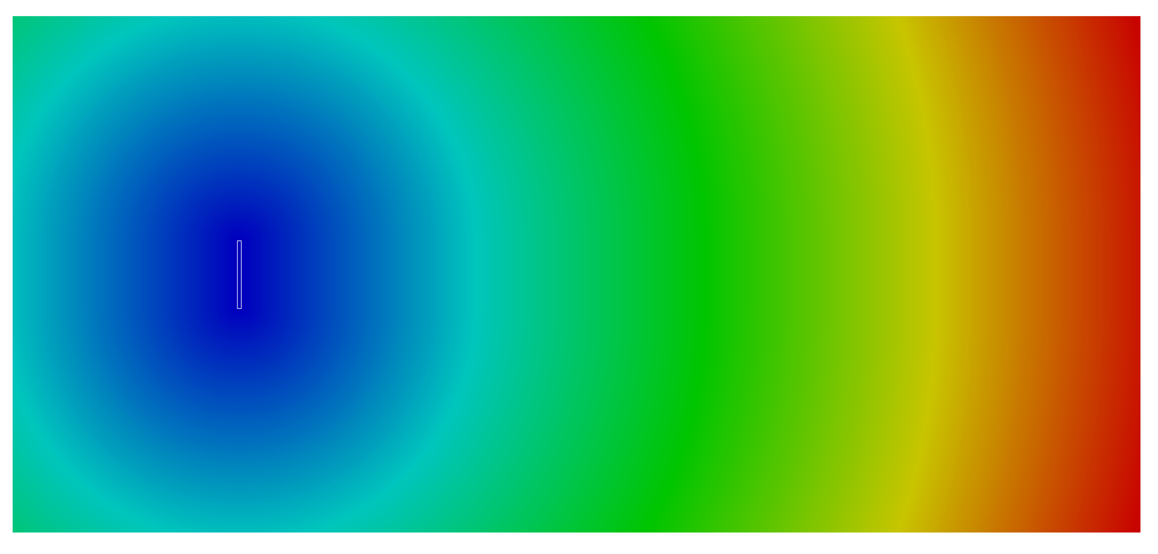
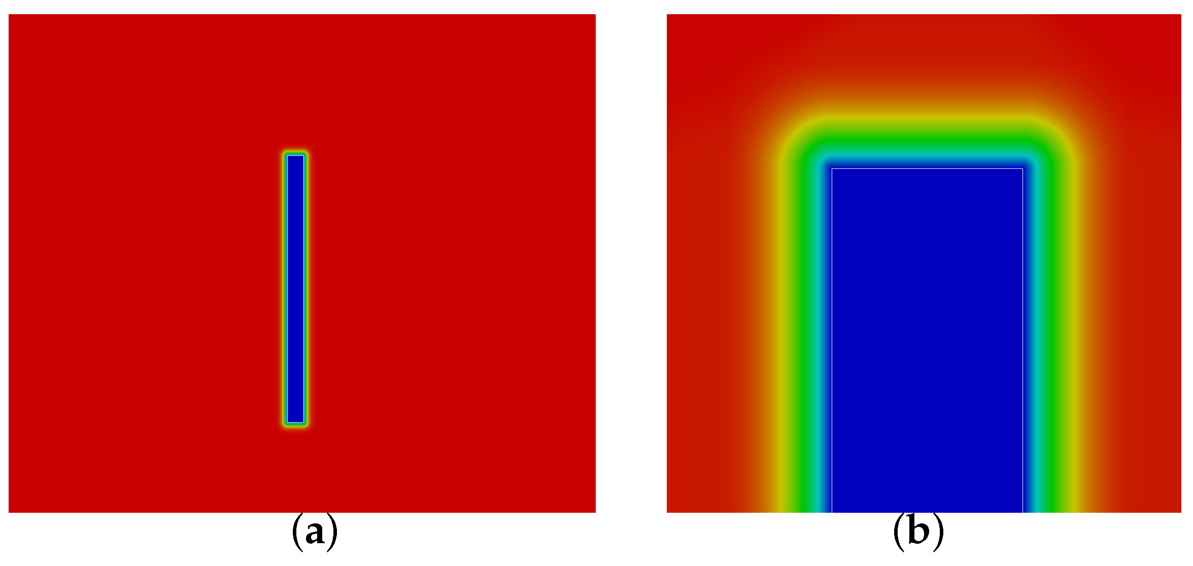
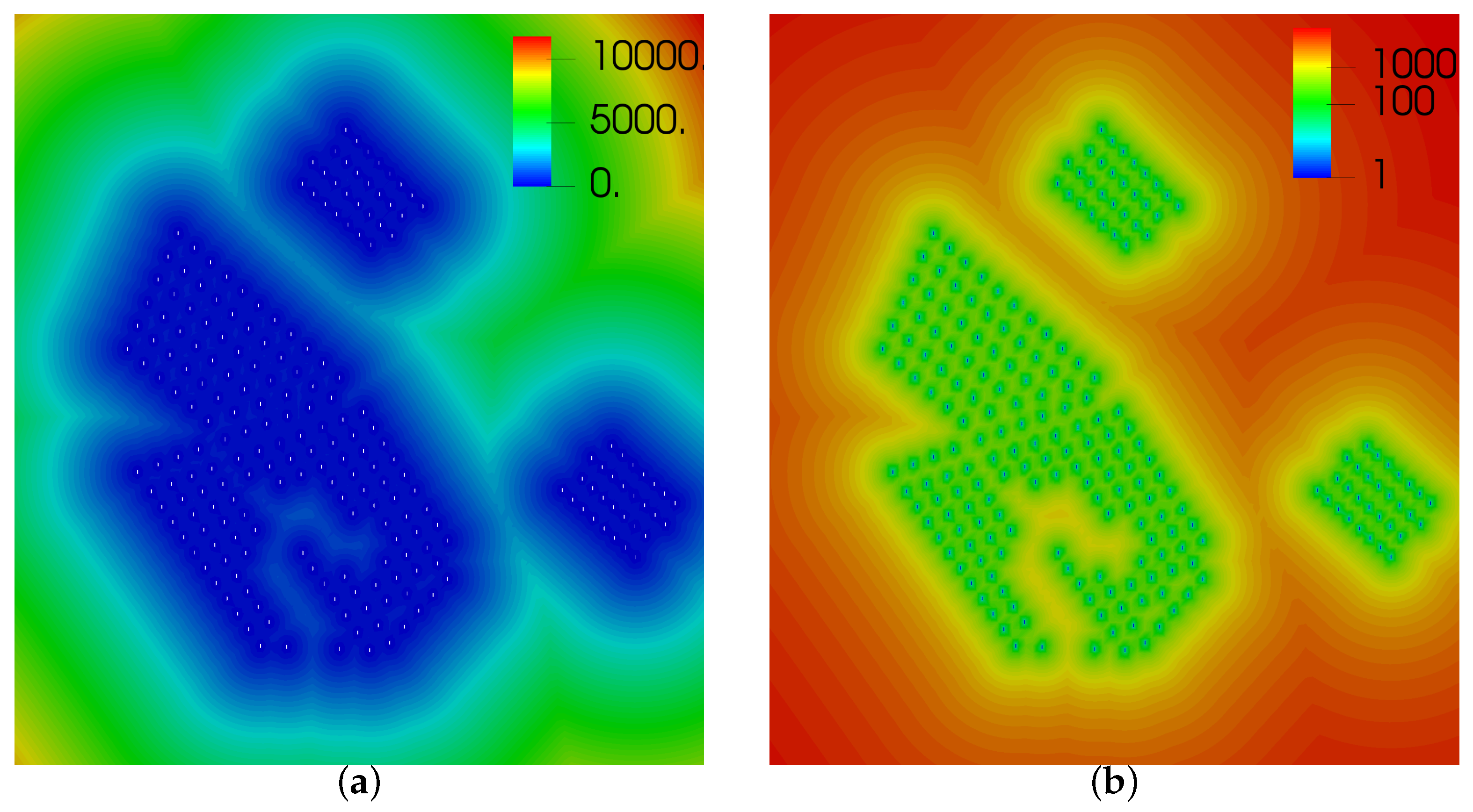
Figure 3 illustrates the level set function—see Equation (2)—for a single turbine test case, corresponding to the distance for each point of the domain to the actuator disc. Figure 4 illustrates the corresponding interface function ($E=1$)—see Equation (3). In addition, Figure 5a shows the level set function for the case of four neighboring wind farms on the North Sea composed by a total of 219 turbines. Figure 5b shows the level set function in logarithmic scale for this wind farm, which illustrates the scales of the problem, ranging from 0 to 12km. 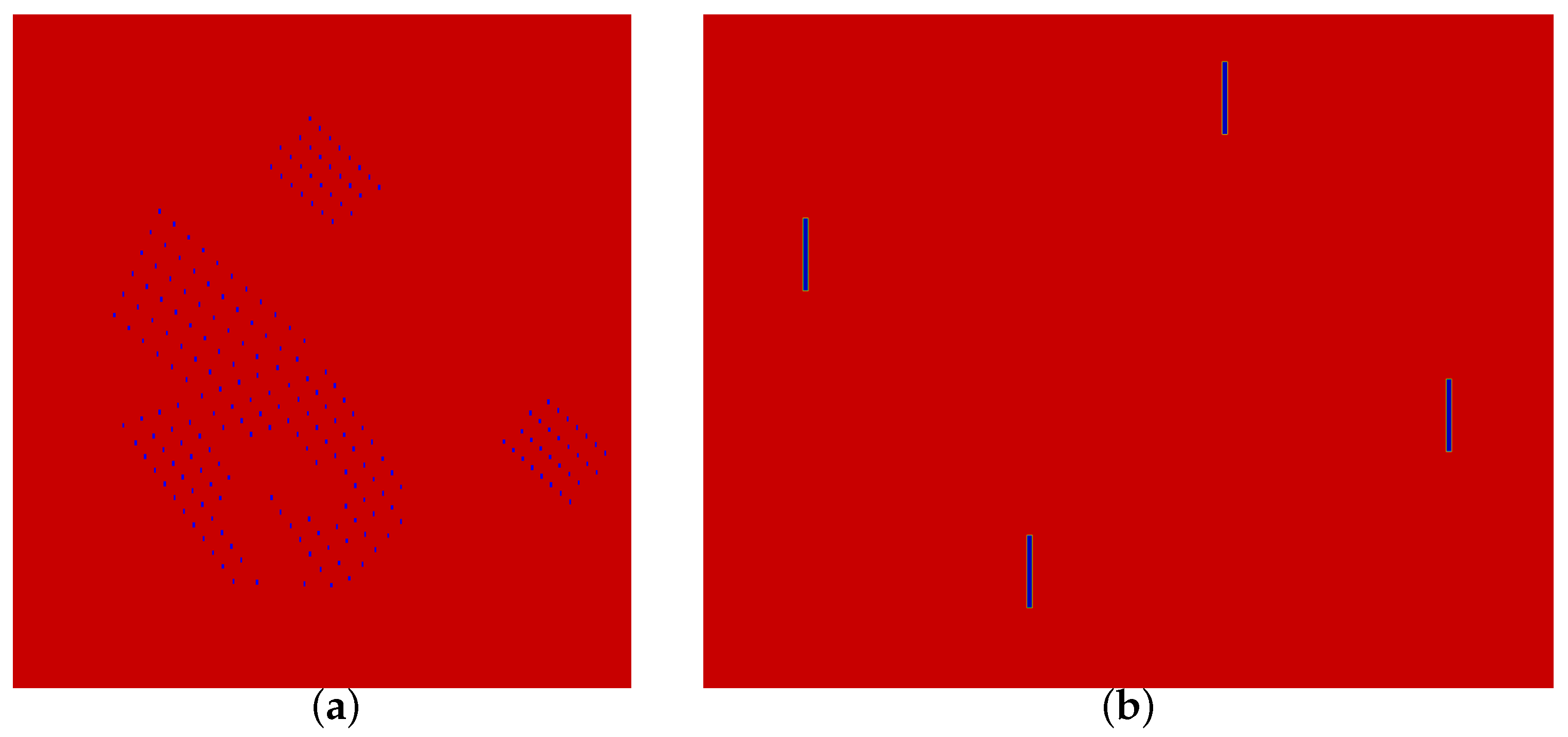The interface function ($E=1$) for the North Sea case is illustrated in Figure 6a, whereas Figure 6b shows a closeup to four turbines. Close to each of the 219 turbines, the interface function behaves analogously to Figure 4.

In Figure 4 and Figure 6, it can be observed that the interface function is almost constant inside and outside the discs, and features a high-variation close to the discs. As detailed in [30], the transition region where the variation of the interface function is produced is determined by the parameter E. Thus, adapting the mesh to capture this interface provides a disc discretization precise up to the desired discretization size, whereas the rest of the domain can be discretized with a larger mesh size. Next, Section 3.2 presents the adaptive process to generate a mesh adapted to this level set actuator disc representation. Using this boundary representation and the adaptive meshing process, finally in Section 3.3, the optimal value of the E parameter is devised, and the convergence of the generated meshes to the exact actuator disc region is validated.

3.2. Actuator Disc Discretization Using a Metric-Driven Adaptation Process

In this section, our approach to generate a mesh adapted to a given turbine configuration is presented. This mesh for simulation is based on an adaptation process to capture the interface function presented in Equation (3). The mesh is devised to discretize with the desired mesh size the level set geometry representation. In Section 5, this mesh constitutes the starting point of an adaptive cycle to capture both the geometry and current flow solution.

Following the ideas presented in [31,32,34], from the Hessian ${\mathcal{H}}_f$ of the interface function at a given point, the interface metric is defined as:

$${\mathcal{M}}_{\mathbf{f}}={\mathbf{V}}_{\mathbf{f}}{\mathbf{D}}_{\mathbf{f}}{\mathbf{V}}_{\mathbf{f}}^t,$$

(4)

where ${\mathbf{V}}_{\mathbf{f}}$ is the matrix composed by the eigenvectors of ${\mathcal{H}}_f$, and ${\mathbf{D}}_{\mathbf{f}}$ a diagonal matrix with the absolute value of its eigenvalues. From ${\mathcal{M}}_{\mathbf{f}}$ a new metric that can be discretized with approximately N nodes can be defined [34,35]:

$${\mathcal{M}}_f^N:={\left(\frac{N}{\mathcal{C}\left({\mathcal{M}}_{\mathbf{f}}\right)}\right)}^{\frac{2}{d}}{\mathcal{M}}_{\mathbf{f}},$$

(5)

which is denoted herein as target interface metric, and where $\mathcal{C}\left({\mathcal{M}}_{\mathbf{f}}\right)$ is the metric complexity:

$$\mathcal{C}\left(\mathcal{M}\right):={\int }_{\mathsf{\Omega }}\sqrt{det\mathcal{M}\left({\mathbf{x}}_{}\right)}d{\mathbf{x}}_{}.$$

(6)

In addition to having control over the number of nodes of the mesh compliant with our metric, herein we also aim to control the minimum ($h_{min}$) and maximum ($h_{max}$) mesh size. To achieve this, according to [32], we impose a lower and upper bound of the eigenvalues of the resulting metric. The minimum metric eigenvalue is bounded by $h_{max}^{-2}$, and the maximum eigenvalue by $h_{min}^{-2}$. In addition, in this work, for simplicity we aim to obtain isotropic meshes by means of defining a diagonal eigenvalue matrix ${\mathbf{D}}_{\mathbf{f}}$ in Equation (4) featuring the minimum of the two positive eigenvalues.

Given a target metric, lengths and areas are measured according to it. Ideally, all the entities of a mesh should have unit measure according to the desired metric. However, in general due to the topological constraints this can not be achieved. Thus, this condition is relaxed [25] and a quasi-unitary mesh is desired, that is, a mesh with edges lengths in the range $\left[\frac{1}{\sqrt{2}},\sqrt{2}\right]$. To obtain a quasi-unitary mesh from a given mesh, a set of topological and optimization operations has to be performed—see [25,30,32,33,43,44] for a review of adaptive meshing strategies. In this work, the mesh topology adaptation is cast to the software BAMG [44].

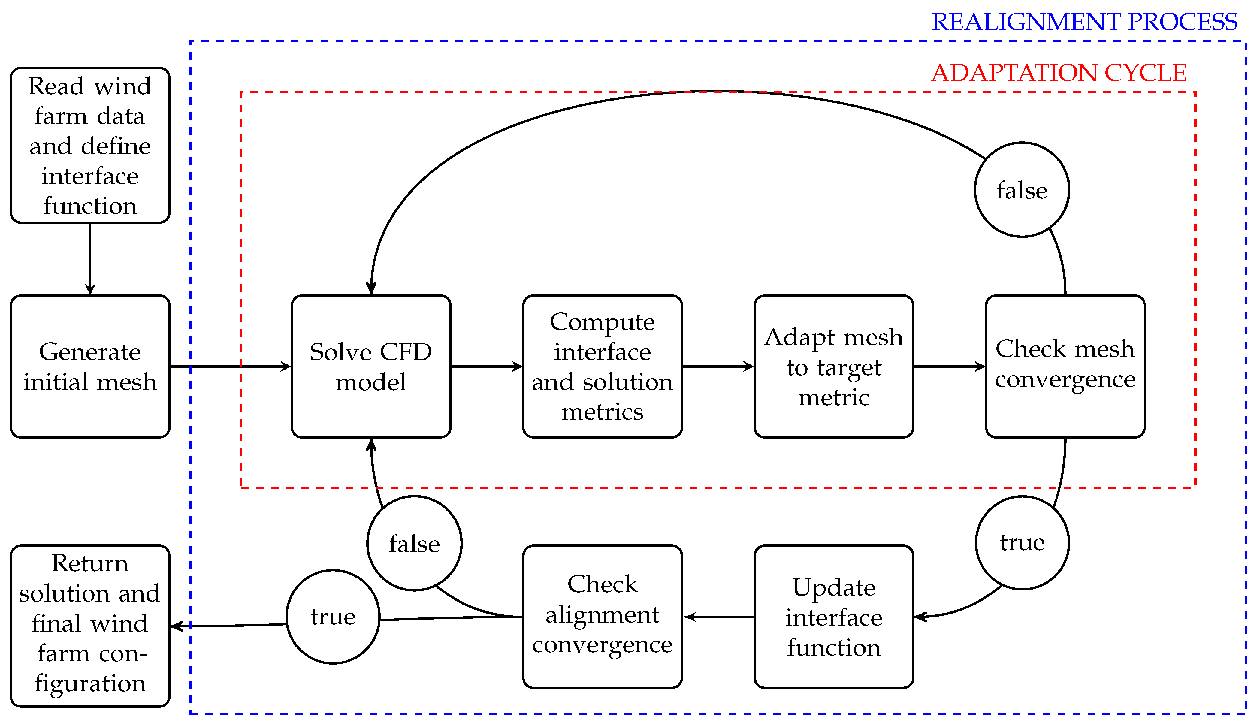
Taking into account the desired target metric, Algorithm 1 details the proposed adaptivity process to generate an initial mesh adapted to the actuator disc model of a given wind farm. The starting point of the actuator disc meshing process features an initial mesh that captures the location of the turbines. To achieve this, in Line 3 a mesh featuring the boundary of the target domain $\mathsf{\Omega }$ is generated, which includes the corners and hub center of the actuator discs ${\left\{{\mathsf{\Omega }}_i\right\}}_{i=1}^{n_t}$. A uniform background mesh of a fine size can also be generated, although the cost and required number of degrees of freedom is increased. Given the initial mesh, where a point in each actuator disc must be ensured to detect the interface function of the discs, the adaptation process (Line 5) to capture the level set geometry is started. To achieve this, the Hessian of the interface function on the mesh nodes is evaluated, from which the target metric is computed, Line 7, according to Equations (4) and (5). Recall that the metric is modified to comply with the desired complexity, and to respect the desired minimum and maximum mesh sizes.

Algorithm 1 Generation of the a mesh adapted to the actuator disc representation of a wind farm.

Input: Target domain $\mathsf{\Omega }$, Actuator discs ${\left\{{\mathsf{\Omega }}_i\right\}}_{i=1}^{n_t}$ Number of desired nodes N, Maximum edge length $h_{max}$, Minimum edge length $h_{min}$ Output: Mesh adapted to discs M 1: function GenerateDiscMesh($\mathsf{\Omega }$, ${\left\{{\mathsf{\Omega }}_i\right\}}_{i=1}^{n_t}$, N, $h_{max}$, $h_{min}$) 2:  $i\leftarrow 0$ 3:  $M_0$← GenerateInitialMesh( $\mathsf{\Omega }$, ${\left\{{\mathsf{\Omega }}_i\right\}}_{i=1}^{n_t}$) 4:  isConverged ← false 5:  while not isConverged do 6:    f← SetInterfaceFunction( $\mathsf{\Omega }$, ${\left\{{\mathsf{\Omega }}_i\right\}}_{i=1}^{n_t}$ ) 7:    ${\mathcal{M}}_{\mathbf{f}}^i\leftarrow$ ComputeMetric( f, N, $h_{max}$, $h_{min}$ ) 8:    $M_{i+1}$←AdaptMeshToMetric( $M_i$, ${\mathcal{M}}_{\mathbf{f}}^i$ ) 9:    isConverged ← ($M_i\simeq M_{i+1}$&$i<i{t}_{max}$) 10:   $i\leftarrow i+1$ 11:  end while 12:  $M\leftarrow M_i$ 13:  return M 14: end function

Once the desired metric is obtained, the mesh is adapted to comply with it, Line 8. The adaptation process finalizes when the new generated mesh has not undergone sufficient mesh modification with respect to the previous one. In particular, the adaptation is stopped, Line 9, when less than $1\%$ of elements and nodes are modified. To ensure the finalization, a maximum of $i{t}_{max}$ iterations is allowed. Herein the maximum allowed is 100, although for all the tested cases the process finalizes in at most five iterations (case in Figure 5).

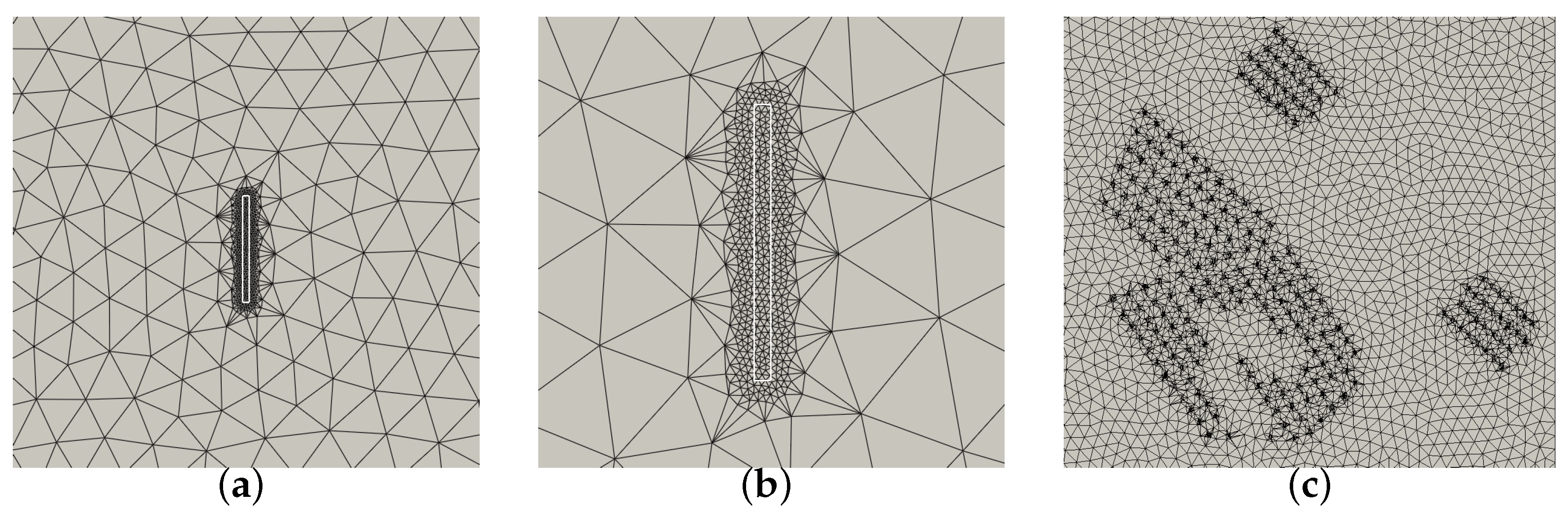
Figure 7a illustrates the mesh generated for a single onshore turbine featuring a diameter of 60 m. The minimum and the maximum mesh size are 1 m and 25 m, respectively. The target number of nodes is 5000, but the generated mesh features 2224. Figure 7c illustrates the case of four neighboring wind farms located on the North sea, featuring 219 turbines with a diameter of 120 m. For illustration purposes, the minimum and the maximum mesh size are 7 and 500 m, respectively. The target number of nodes are 100 K, but the generated mesh features 78 K. In both cases, the obtained number of nodes is lower than the target one. This is due to the fact that in these cases, to attain the number of target nodes, the mesh size should be lower than the required one. Thus, to avoid obtaining a mesh size lower than desired, the minimum mesh size demanded by the metric is limited.

In practice, the meshes generated using this interface function provide a good starting point for the adaptive simulation cycle presented in Section 5. They have the sufficient accuracy to discretize the actuator discs, but they are coarse in the rest of the domain (according to the desired maximum size) to avoid having a high computation cost before being adapted to the actual flow configuration—see details in Section 5.

3.3. Selection of the Interface Parameter and Convergence to the Disc

In the interface function, Equation (3), the parameter E controls the width and sharpness of the interface [30]. Analyzing Equation (3), this parameter divides the distance function before applying the hyperbolic tangent. Thus, herein we can interpret it as a parameter relative to the width of the interface. Due to the behavior of the hyperbolic tangent, E is approximately half the width of the interface.

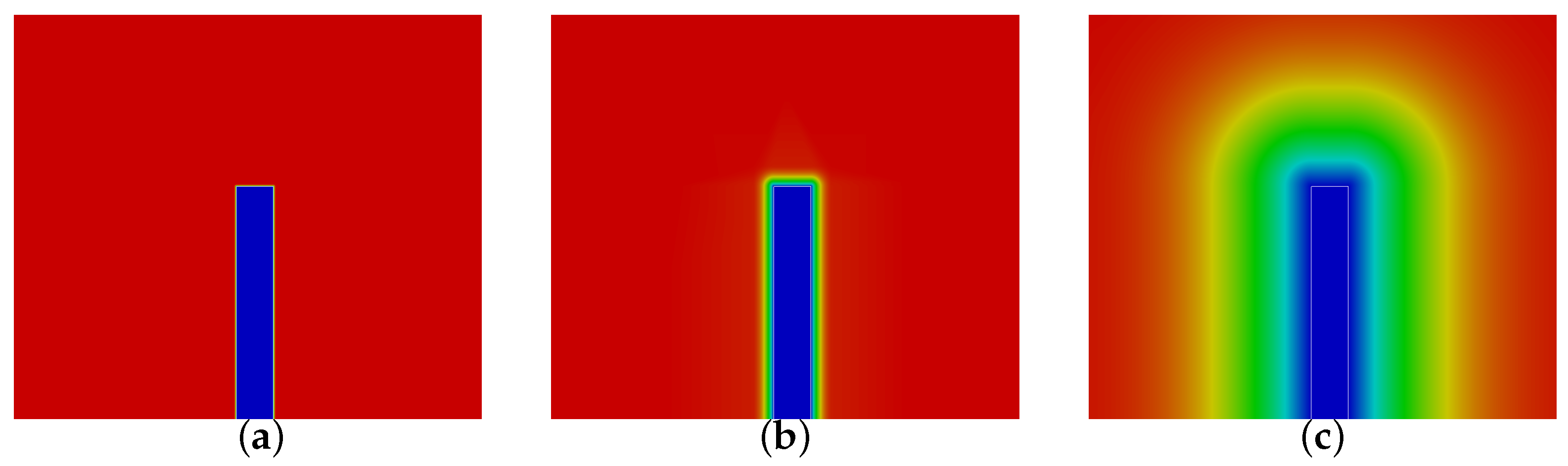
In [30], only values of E greater than or equal to one are considered. However, our analysis takes into account positive values lower than one to check all feasible values for the interface definition of the actuator discs. Figure 8 illustrates values 0.1, 1 and 10 of parameter E of the interface function. Analyzing the three illustrated values, $E=0.1$ provides a sharp interface, which is enlarged for $E=1$ and further extended for $E=10$. It can be observed that values lower than one sharpen the interface, whereas greater values enlarge it.

By strictly observing the interface, our choice among these three would be $E=1$. Measuring the interface, it can be observed that it has a width of 2 m, which is approximately half the disc width. This interface length is of the order of the mesh size that would be reasonable to discretize the disc, and thus it could be captured with the desired mesh size. In contrast, on the one side, the interface of $E=0.1$ is of $0.2$ m, which is significantly small compared to the target mesh size and to the large scales (kilometers) of the problem to be solved. On the other side, the interface for $E=10$ has 20 m, which will extend the region of refinement excessively away from the disc. One of the desired features of the initial mesh is that it does not over-refine the domain. In contrast, the target is to obtain an initial mesh that is valid for simulation, discretizing the actuator disc and that will later be refined according to the actual flow requirements.

Following, the choice of the parameter is further analyzed, taking into account the accuracy on the actuator disc region induced by different values of the parameter, and also the required degrees of freedom to represent it. To achieve this, a sequence of meshes for $E=[0.1,20]$ are generated for the scenarios in Figure 7a (case featuring one turbine) and Figure 7c (case featuring 219 turbines). Fixing the same maximum ($h_{max}=1D_{}$) and minimum ($h_{min}=0.5{\mathsf{\Delta }}_{}$) mesh size, the relative error of the disc area is computed. 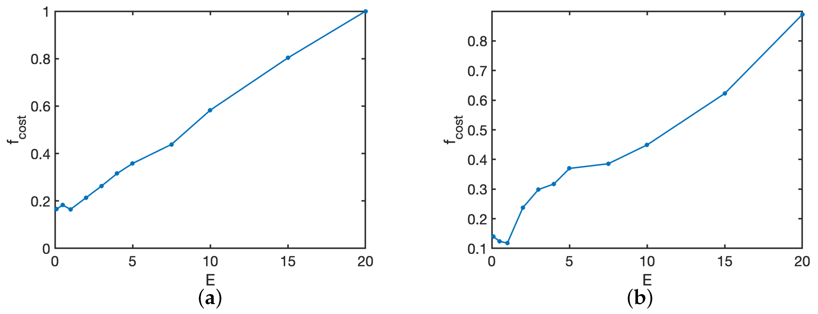Figure 9 illustrates a target cost function to determine a reasonable value of E for the two different tested cases. In particular, the target cost function $f_{cost}$ is defined as the product of the relative error (normalized by the maximum error) by the number of generated nodes (normalized by the maximum number of nodes). For a fixed mesh size, the objective of the designed cost function is to avoid any value of E that gives a bad region approximation, but to favor the lowest element count for values providing a similar accuracy.

For the two configurations in Figure 9, $E=1$ delivers the minimum cost, presenting the best balance between accuracy and computational cost. Thus, for the rest of the work E is set as 1. This analysis may be different if highly anisotropic meshes where desired, since this parameter also changes the anisotropic ratio normal to the disc boundaries; however, anisotropic meshes are out of the scope of this paper.

We remark that the mesh is not forced to exactly match the boundary of the actuator disc model. Thus, a criterion has to be set to determine the elements that belong to the disc. Herein, the elements with the center of mass on the disc determine the actuator disc region where the sink is imposed. Since the actuator disc is not a geometry but a model, we have actively made the choice to approximate the actuator disc region, taking into account the quadratic convergence of the mesh to the function.

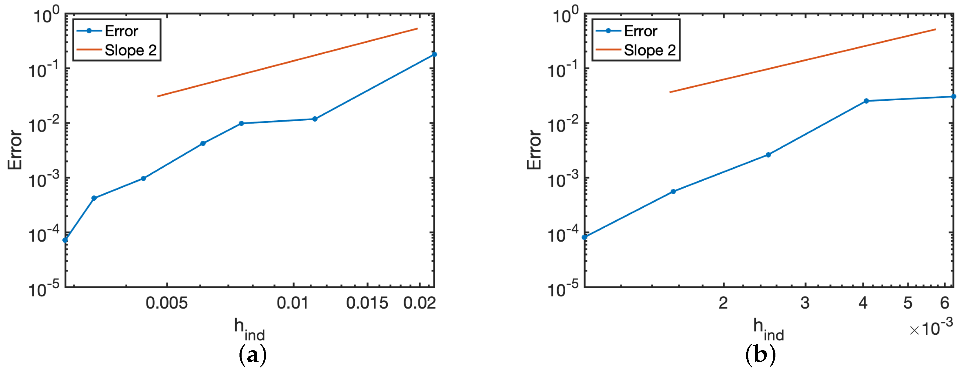
To test the convergence to the actuator disc regions, successively refined meshes are generated, computing the error of the area of the actuator discs for each generated mesh. Figure 10 illustrates a convergence plot of the mesh to the two considered test cases. According to [45], $N^{-1/d}$ is used as an indicator of the mesh size for locally refined meshes, N being the number of nodes of the mesh and d its dimension ($d=2$ for triangles, $d=3$ for tetrahedra). It can be observed that the area convergence of the mesh refinement process outperforms (slope 3.5 for one turbine, 3.4 for the North Sea case) the expected quadratic convergence for a given field. This is so since the area is a quantity of interest resulting from an integral on the mesh. However, it is of valuable for our problem, since this area corresponds to the region where the sink in our equations is imposed.

Taking into account the convergence and accuracy of the mesh to the actuator disc region, we proceed the rest of the work with the proposed definition of the actuator disc elements; however, other choices could be possible. The integration on the interface elements could be enriched to capture their contribution to the source term. Alternatively, projecting the boundaries to the disc is straight-forward in 2D, but demands of mesh repair, projection and optimization tools in 3D, increasing the complexity and overall computational cost—these approaches are out of the scope of the paper. Herein, as previously commented, we restrict to targeting the actuator disc as a function to be discretized and cast the convergence to the disc to the standard convergence properties of the FEM (or equivalently FVM).

4. Convergence Analysis of Standard and Level-Set-Based Approaches

The objective of this section is to validate the level set meshing approach for wind farm simulation. The advantages of this approach have been motivated through the paper, namely: capacity to couple the simulation with an adaptive process, and simplicity to update the geometry according to the flow. However, a possible disadvantage could be that the proposed approach is not boundary tight and, in contrast, the actuator discs are discretized by means of mesh adaptation according to a desired tolerance or mesh size.

In standard wind farm simulation featuring actuator discs [1,5,6,18], the geometry is defined by both the topography and the discs. The actuator discs are not geometric entities (they are not boundaries of the domain) and in contrast introduce a sink in the equations. The objective of this work is to replace considering the disc at the geometry step and consider it as a level set. This section also validates the CFD model for the standard boundary tight case, to have a solution (conformal with the discs), which can be used as reference for the level-set based approach. It must be highlighted that the generation of 3D conformal disc meshes featuring real topographies is a complex problem [1,2,46,47]. In addition, this complexity is increased to perform adaptation, since the solver must be coupled with a geometry kernel to deal with the interaction between mesh and geometry.

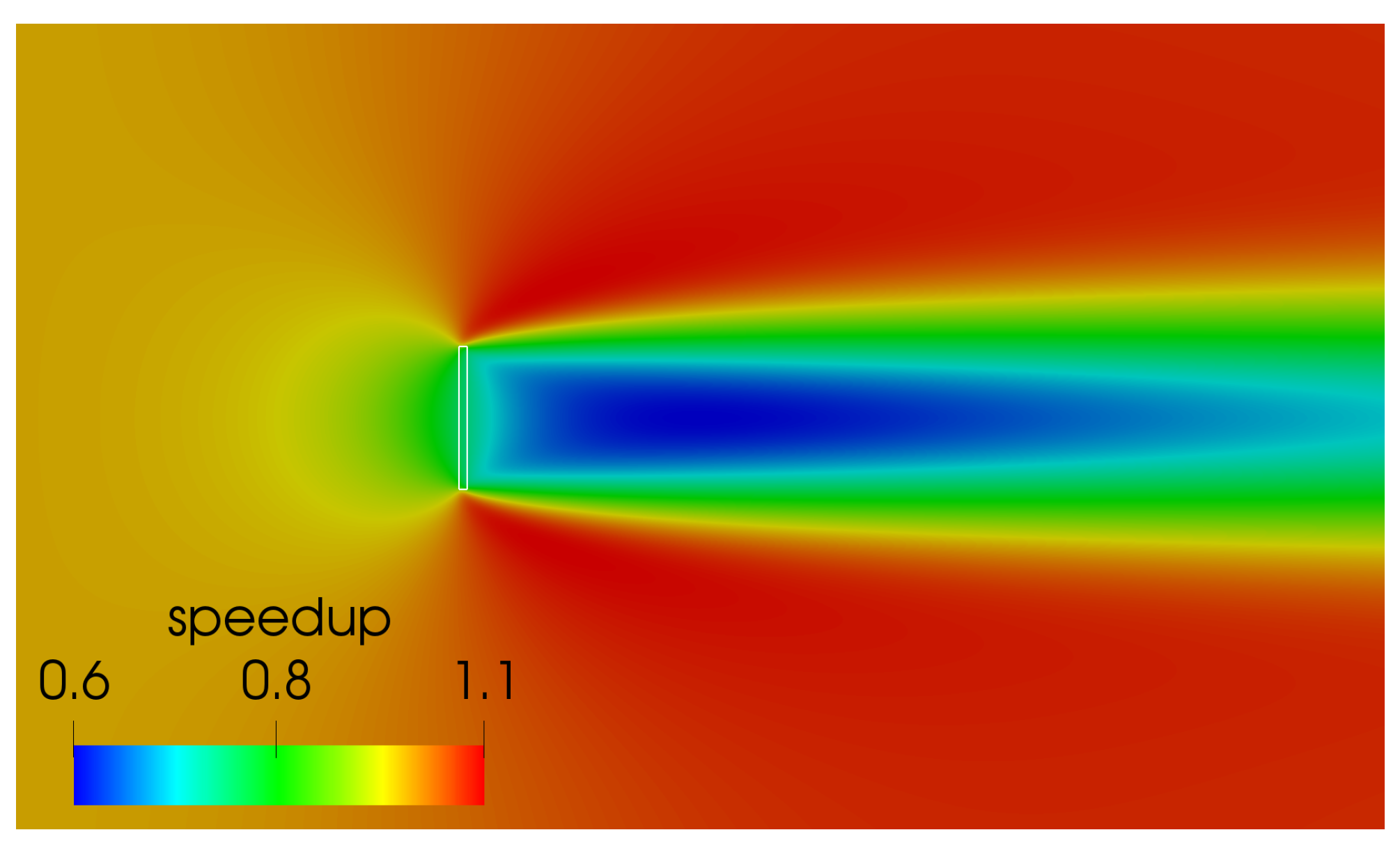
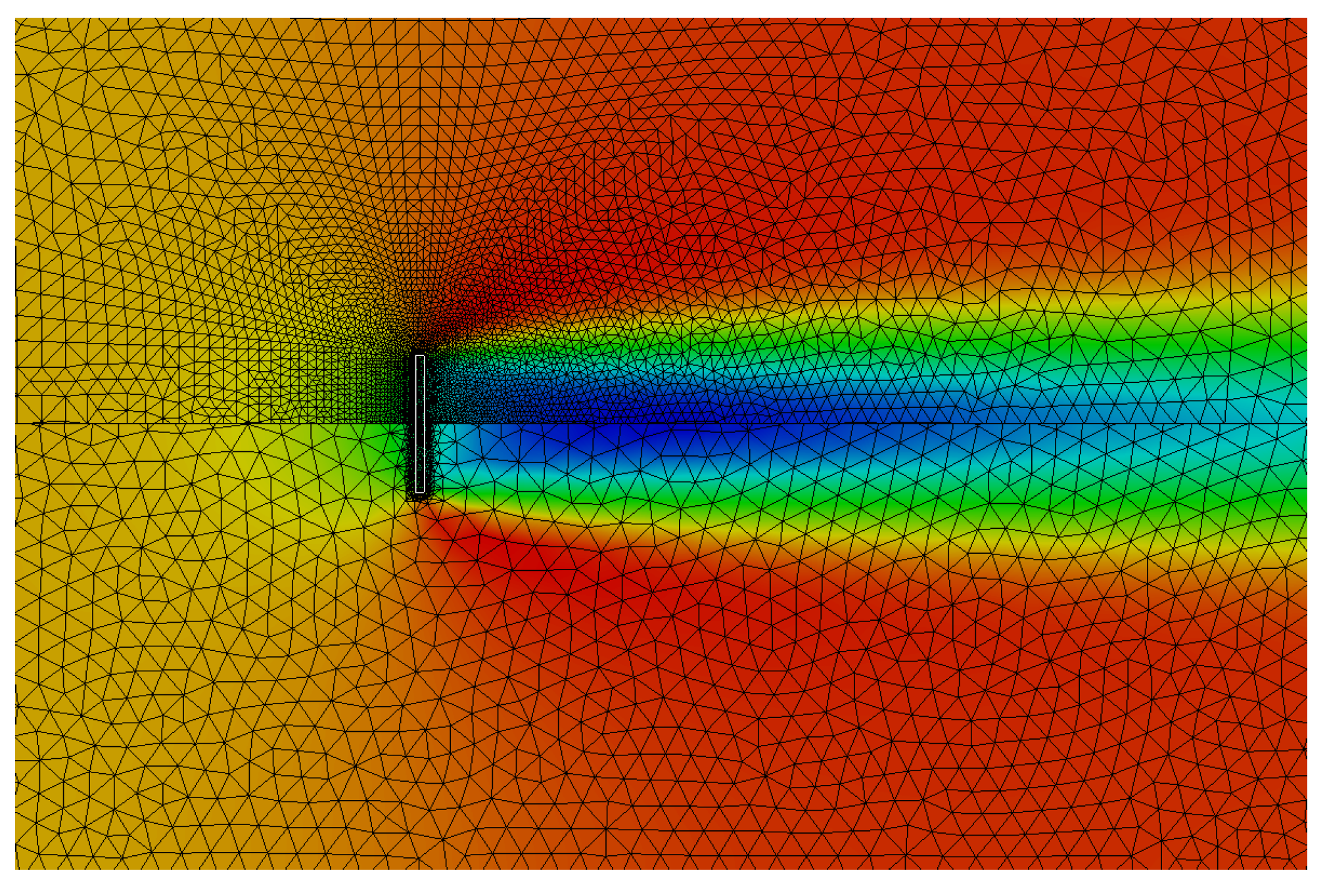
In this section, the boundary tight approach is posed strictly to validate a one case turbine scenario to be used as a reference for the level set approach. Figure 11 illustrates the reference solution meshed conforming to the actuator disc. A 60 m diameter turbine is considered, featuring an actuator disc width of 3.6 m ($6\%D_{}$ [6]). The minimum mesh size at the disc is 0.05 m, and the maximum mesh size on the outer boundary is 1.0 m.

A sequence of refined meshes is generated, starting from a maximum size of 50 m, that is iteratively divided by 2, and a size at the disc of 3.6 m that is analogously refined. For each generated mesh, the solution of our CFD model is computed, calculating the ${\mathcal{L}}^2$-error of the velocity between this solution and a reference solution with the reference mesh. The mesh convergence analysis is performed for both the boundary tight and the level set approach. 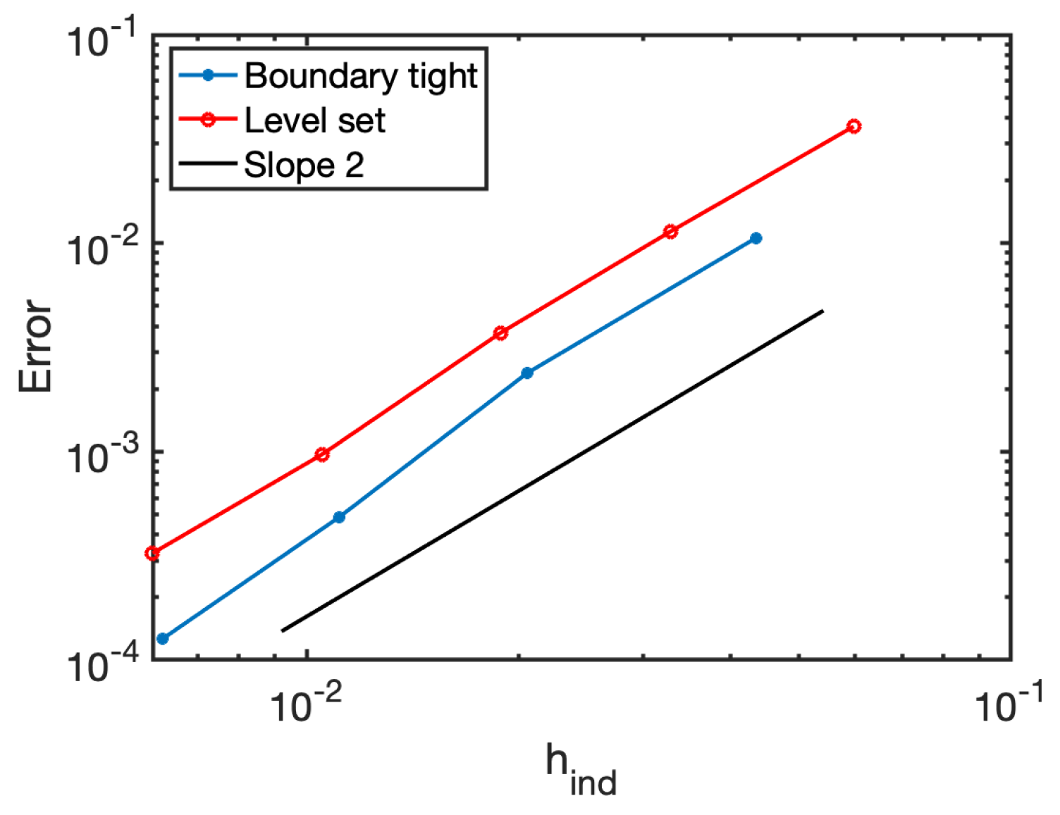Figure 12 shows the obtained convergence plot in logarithmic scale. We use $N^{-1/d}$ as an indicator of the mesh size for locally refined meshes [45], N being the number of nodes of the mesh. As expected, the theoretical quadratic converge is attained.

As it can be observed in Figure 13, in the boundary tight approach the mesh size is imposed on the geometric entities (inner disc and outer boundary) and a linear transition of the mesh size is prescribed. In contrast, in the level set approach the mesh is locally refined to capture the disc, but no size gradation is imposed towards the boundary. Thus, the boundary tight mesh has a smoother size gradation, since in the level set approach the mesh sizing is cast to the adaptation to the solution, as is detailed in Section 5. As a consequence, although both approaches have quadratic convergence, the boundary tight approach has a slight error reduction. As a reference, for the finest meshes, the error of the boundary tight approach is $1.2\times {10}^{-4}$ while the error of the level set one is $3.2\times {10}^{-4}$. If desired, the generated size field could be smoothed by using a metric gradation strategy [48]; however, the mesh sizing is cast to the adaptation to the solution process. An analysis of the convergence of the final adaptive approach is presented in Section 6.1, illustrating the accuracy improvement enabled by the adaptation.

To summarize, we observe that the new approach attains a similar accuracy ($\mathcal{O}\left({10}^{-4}\right)$) and the same convergence behavior. Thus, the level set modeling does not penalize the CFD model and converges with the expected order and to the same solution. Once validated, in Section 5, we present the adaptive simulation process and the turbine realignment approach, which are derived using the level set actuator disc representation.

5. Wind Farm Simulation Featuring Solution Adaptation and Turbine Realignment

In this section, the actuator disc modeling for Section 3 is coupled with a standard adaptation cycle [25,32,33,34,43]. In particular, we detail the specific algorithms involved in the simulation workflow presented in Figure 2 in Section 2.2. First, Section 5.1 details the target metric and the adaptive simulation cycle, framed by a red box in the workflow diagram from Figure 2. Next, in Section 5.2, we present an adaptive wind farm simulation process that features turbine realignment according to the wind flow, framed by a blue box in the workflow diagram from Figure 2.

5.1. Adaptation to the Solution

In standard wind farm simulation [1,2,13,14,16,17,18], the mesh is set a priori based on a well-known behavior of the flow in a wind farm. Further accuracy is required around the turbines, and more specifically, downstream of the turbine. Thus, the standard process steps by generating, based on the practitioner knowledge, a mesh conformal with the discs that is finer upstream and downstream. However, the flow can be over-resolved (loss of computational resources) or under-resolved (loss of precision). This issue is exacerbated by the fact that this a priori setting is based on assuming that the turbines will be aligned according to the inflow, which can not be ensured in general.

One of the advantages of posing a level set actuator disc representation and discretizing it using an adaptive framework, is that this framework can capture simultaneously the solution of our model, determining the mesh according to the flow. Similarly to Section 3, a metric has to be defined incorporating all the necessary information to capture both the discs and the solution. In particular, two functions are taken into account: the interface function and the velocity (magnitude). The interface metric is defined in Equation (4). Similarly, let ${\mathcal{H}}_{\mathbf{u}}$ be the Hessian of the velocity magnitude. Then, the velocity metric is defined as:

$$\begin{array}{ccc}\hfill {\mathcal{M}}_{\mathbf{u}}& =& {\mathbf{V}}_{\mathbf{u}}{\mathbf{D}}_{\mathbf{u}}{\mathbf{V}}_{\mathbf{u}}^t,\hfill \end{array}$$

(7)

where, as detailed for the interface metric, ${\mathbf{V}}_{\mathbf{u}}$ is the matrix with the eigenvectors of the Hessian matrix, and ${\mathbf{D}}_{\mathbf{u}}$ is a diagonal matrix with the absolute value of the eigenvalues.

To take into account the target functions, a new metric complying with both target fields is defined as the intersection of both metrics:

$${\displaystyle {\mathcal{M}}_{\mathit{I}}:={\mathcal{M}}_{\mathit{f}}\cap {\mathcal{M}}_{\mathbf{u}}.}$$

(8)

To conclude, the target metric resolved with N nodes is defined as

$$\mathcal{M}:={\left(\frac{N}{\mathcal{C}\left({\mathcal{M}}_{\mathit{I}}\right)}\right)}^{\frac{2}{d}}{\mathcal{M}}_{\mathit{I}},$$

(9)

where $\mathcal{C}\left(\mathcal{M}\right)$ is the complexity of the metric—see Equation (6). It must be pointed out that, in addition to the velocity magnitude, any other additional target solution could be targeted (for instance, the pressure field), by means of defining the corresponding metric (${\mathcal{M}}_{\mathit{p}}$ analogously to Equation (7)), and intersecting with the interface and velocity ones in Equation (8).

The adaptive framework is detailed in Algorithm 2. As previously commented, the starting point (Line 3) is the mesh adapted to the input disc configuration presented in Section 3.2—see Algorithm 1. Given a mesh, the solution of the CFD model presented in Section 2.1 is computed—see Line 6. Next, the target metric with the desired complexity is computed—see Line 7. Given a mesh and a metric, the mesh is adapted to the metric in Line 8. If the new mesh is converged with respect to the previous one the process is finalized. Otherwise, taking into account the current solution as initial condition, a new solution of the model is computed, repeating the adaptive process until convergence. Similarly to Algorithm 1, herein the process is considered to be converged when less than $1\%$ of elements and nodes are modified.

Algorithm 2 Adaptive simulation of a wind farm.

Input: Target domain $\mathsf{\Omega }$, Actuator discs ${\left\{{\mathsf{\Omega }}_k\right\}}_{k=1}^{n_t}$, Number of desired nodes N, Maximum edge length $h_{max}$, Minimum edge length $h_{min}$ Output: Adapted mesh M, Velocity $\mathbf{u}$, Pressure p 1: function AdaptiveWindFarmSimulation( $\mathsf{\Omega }$, ${\left\{{\mathsf{\Omega }}_k\right\}}_{k=1}^{n_t}$, N, $h_{max}$, $h_{min}$ ) 2:  $i\leftarrow 0$ 3:  $M_0$←GenerateDiscMesh( $\mathsf{\Omega }$, ${\left\{{\mathsf{\Omega }}_k\right\}}_{k=1}^{n_t}$, N, $h_{max}$, $h_{min}$ ) 4:  isConverged ← false 5:  while not isConverged do 6:    $\mathbf{u},p$← SolveWindModel( $M_i$ ) 7:    $\mathcal{M}\leftarrow$ ComputeTargetMetric( $M_i$, $\mathbf{u}$, p, ${\left\{{\mathsf{\Omega }}_k\right\}}_{k=1}^{n_t}$, N, $h_{max}$, $h_{min}$ ) 8:    $M_{i+1}$← AdaptMeshToMetric( $M_i$, $\mathcal{M}$ ) 9:    isConverged ← ( $M_i\simeq M_{i+1}$&$i<i{t}_{max}$ ) 10:   $i\leftarrow i+1$ 11:  end while 12:  $M\leftarrow M_i$ 13:  return M, $\mathbf{u}$, p 14: end function

5.2. Adaptation and Realignment with the Flow

This section presents one of the main advantages derived from the level set representation of the actuator disc model for wind farm simulation: the capacity to update the turbine configuration according to the actual wind direction. The flexibility provided by the defined level set representation of the actuator discs—see Section 3—is herein exploited to successively redefine the level set to align the actuator discs with the wind direction.

Algorithm 3 details the algorithm corresponding to the adaptive simulation cycle with actuator disc realignment. It can be observed that it is composed by two loops. The inner one, Lines 8–14, is analogous to the adaptation algorithm presented in Section 5.1—see Algorithm 2. Given an initial mesh, while the mesh is modified, we simulate and adapt the mesh to the actual flow solution. Now, an external loop is added, checking the convergence of the actuator disc level set model, Lines 5–8 and 14–19. The difference between both algorithm lies in the fact that once the simulation is converged, Line 14, the level set geometry is updated to comply the current state of the flow, Line 15. In particular, the turbines are realigned according to the flow, and the level set function is updated.

As detailed in Section 3.1, the level set geometry is defined as a rectangle region centered on the turbine hub, with one side equal to the diameter of the turbine and the other according to the actuator model thickness ($6\%$ of the diameter [6]). This rectangle is oriented according to a given normal ${\mathbf{n}}_{\mathbf{i}}\in {\mathbb{R}}^2$. Hence, in Line 15, given a flow solution, the level set geometry is redefined according to a normal taking into account the actual flow configuration. In particular, the normal ${\mathbf{n}}_{\mathbf{i}}$ for the ith turbine ${\mathsf{\Omega }}_i$ is updated according to the mean velocity at the actuator disc.

$${\mathbf{n}}_{\mathbf{i}}=-\frac{{\mathbf{u}}_{\mathbf{i}}}{∥{\mathbf{u}}_{\mathbf{i}}∥},$$

where

$${\mathbf{u}}_{\mathbf{i}}:=\frac{1}{|{\mathsf{\Omega }}_i|}{\int }_{{\mathsf{\Omega }}_i}\mathbf{u}\mathrm{d}\mathsf{\Omega },$$

is the mean velocity on the disc, where $|{\mathsf{\Omega }}_i|$ is the area of the disc.

Modifying the level set function has three main implications. First, it changes the actuator disc term in the CFD model—see Equation (1). The normal of the actuator discs is modified and thus, the momentum sink changes accordingly, and so the solution does too. Second, the level set function determines where the actuator disc source term is applied, changing again the equation and the solution. Third, the level set function is taken into account in the mesh adaptation—see Equation (8). Updating the level set, modifies its metric, which produces a change in the mesh adaptation process. These three effects require the existence of an outer loop that iterates until the level set model is converged.

Algorithm 3 Adaptive simulation of a wind farm with turbine realignment.

Input: Target domain $\mathsf{\Omega }$, Actuator discs ${\left\{{\mathsf{\Omega }}_k\right\}}_{k=1}^{n_t}$, Number of desired nodes N, Maximum edge length $h_{max}$, Minimum edge length $h_{min}$ Output: Adapted mesh M, Velocity $\mathbf{u}$, Pressure p 1: function WindFarmSimulationWithRealignment($\mathsf{\Omega }$, ${\left\{{\mathsf{\Omega }}_k\right\}}_{k=1}^{n_t}$, N, $h_{max}$, $h_{min}$) 2:  $j\leftarrow 0$ 3:  $M_0$←GenerateDiscMesh($\mathsf{\Omega }$, ${\left\{{\mathsf{\Omega }}_k\right\}}_{k=1}^{n_t}$, N, $h_{max}$, $h_{min}$) 4:  isConvergedDiscModel ← false 5:  while not isConvergedDiscModel do 6:    $i\leftarrow 0$ 7:    isConvergedCFD ← false 8:    while not isConvergedCFD do 9:     $\mathbf{u},p$← SolveWindModel($M_i$) 10:    $\mathcal{M}\leftarrow$ ComputeTargetMetric($M_i$, $\mathbf{u}$, p, ${\left\{{\mathsf{\Omega }}_k\right\}}_{k=1}^{n_t}$, N, $h_{max}$, $h_{min}$) 11:     $M_{i+1}$← AdaptMeshToMetric($M_i$,$\mathcal{M}$) 12:     isConvergedCFD ← ($M_i\simeq M_{i+1}$&$i<i{t}_{max}^{CFD}$) 13:     $i\leftarrow i+1$ 14:    end while 15:    ${\left\{{\mathsf{\Omega }}_k^{new}\right\}}_{k=1}^{n_t}$ ← UpdateDiscModel(${\left\{{\mathsf{\Omega }}_k\right\}}_{k=1}^{n_t}$,$\mathbf{u}$) 16:    isConvergedDiscModel ←$\left({\left\{{\mathsf{\Omega }}_k^{new}\right\}}_{k=1}^{n_t}\simeq {\left\{{\mathsf{\Omega }}_k\right\}}_{k=1}^{n_t}\&j<i{t}_{max}^{disc}\right)$ 17:    ${\left\{{\mathsf{\Omega }}_k\right\}}_{k=1}^{n_t}$←${\left\{{\mathsf{\Omega }}_k^{new}\right\}}_{k=1}^{n_t}$ 18:    $j\leftarrow j+1$ 19:  end while 20:  $M\leftarrow M_i$ 21:  return M, $\mathbf{u}$, p 22: end function

6. Results

This section validates the proposed methods and presents their application to several scenarios. First, in Section 6.1 the convergence and accuracy of the adaptive simulation framework for a single case turbine is analyzed. Section 6.2 illustrates the case of a set of four neighboring wind farms located on the North Sea, adapting the mesh to a configuration featuring 219 turbines. Next, in Section 6.3, a single turbine case is presented to validate the realignment according to the flow direction. Finally, in Section 6.4 the realignment process is applied to a wind farm featuring 115 turbines.

The 2D CFD model is implemented in Matlab [49], and the topological mesh adaptation is performed using BAMG [44]. All simulations have been computed in a MacBook Pro with one dual-core Intel Core i7 CPU, a clock frequency of 3.0 GHz and a total memory of 16 GBytes. The simulation time ranges from a few minutes in Section 4, Section 6.1 and Section 6.3, to a few hours for Section 6.2 and Section 6.4, depending on the desired mesh size, the size of the domain and the demanded convergence tolerance.

6.1. Convergence Analysis of the Adaptive Simulation Process

In this section, the convergence and accuracy of the adaptive simulation framework is validated. A sequence of meshes analogous to the ones in Section 4 is generated. From a maximum and minimum mesh size from 50 m and 3.6 m, we successively divide them by two. We simulate adapting the mesh to the flow, according to Algorithm 2, and measuring the accuracy with respect to the reference mesh from Section 4. Figure 14 shows in logarithmic scale the velocity error against the size indicator $N^{-2}$ [45], where N is the number of nodes of the mesh.

It can observed that the adaptive process preserves the expected quadratic convergence. The error is reduced over an order of magnitude with respect to the two approaches from Section 4, where uniform refinement was imposed. This is one of the main advantages obtained from using adaptation, the increase in accuracy with respect to meshes with analogous number of degrees of freedom. In addition, as observed for uniform refinement in Section 4, the level set adaptive based approach converges to the solution of the standard boundary tight simulation, validating the obtained solution.

Although adaptivity can also be enabled in geometry-conformal approaches, it involves significantly complex operations to keep the conformity to the geometry. In particular, the solver needs access to the geometry, and a geometry kernel needs to be coupled with the solver to deal with projections to the geometry, while the adaptive topological operations need to be aware of the boundary elements. In contrast, in this work, this issue is prevented by embedding the geometry constrains to the target metric to perform the adaptation, not losing accuracy with respect to the body-tight representation, and coupling adaptation to the actuator discs and to the solution in a single (geometry projection-free) adaptation process.

6.2. Simulation of Four Neighboring Wind Farms: 219 Turbines

The objective of this section is to show the application of the adaptive simulation process to a set of four neighboring wind farms located in the North Sea. The simulation involves 219 turbines of four different models, all featuring a diameter of 120 m. A fixed turbine configuration is simulated, and thus, in the simulation process only refinement to capture the solution is performed. The level set model is kept fixed (without realignment) and Algorithm 2 is used to perform the simulation.

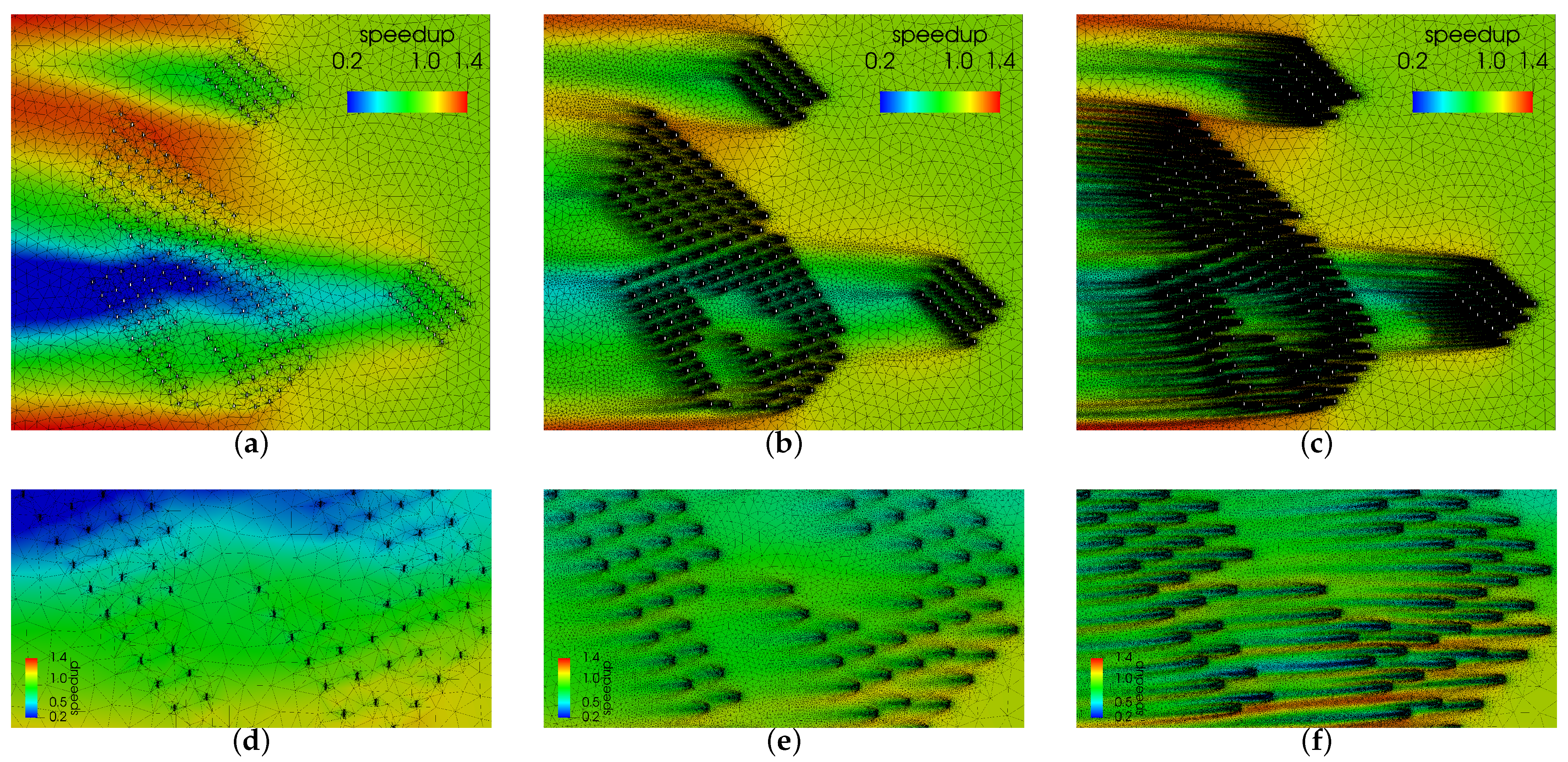
Figure 15 shows an overview of the initial, intermediate and final obtained meshes. In the meshing process, a minimum mesh size of 3.6 m and a maximum size of 500 m are imposed. The complexity of the target metric is set to obtain a mesh of at most 750 K nodes, limited by the prescribed minimum and maximum mesh size. The initial mesh, generated to discretize the level set model is illustrated in Figure 15a, and is composed of 39 K nodes 78 K triangles. The adaptation process takes 15 iterations to converge. The intermediate step is illustrated in Figure 15b, featuring 232 K nodes and 463 K triangles. The final mesh, Figure 15c, is composed of 651 K nodes and 1.3 M triangles.

It can be observed that during the simulation process the adaptation has devised a non-uniform mesh refined to capture the flow features. This is one of the advantages of the current presented modeling approach, since in standard wind farm frameworks, a fine mesh expands uniformly from the turbines to ensure that everywhere the resolution is sufficient. Herein, in contrast, in Figure 15f it can be observed that downstream the turbines, the mesh is not uniform, and regions with higher velocity changes feature smaller mesh size. The size is prescribed according to the actual flow, and taking into account the complex interactions of the turbines of the wind farm. 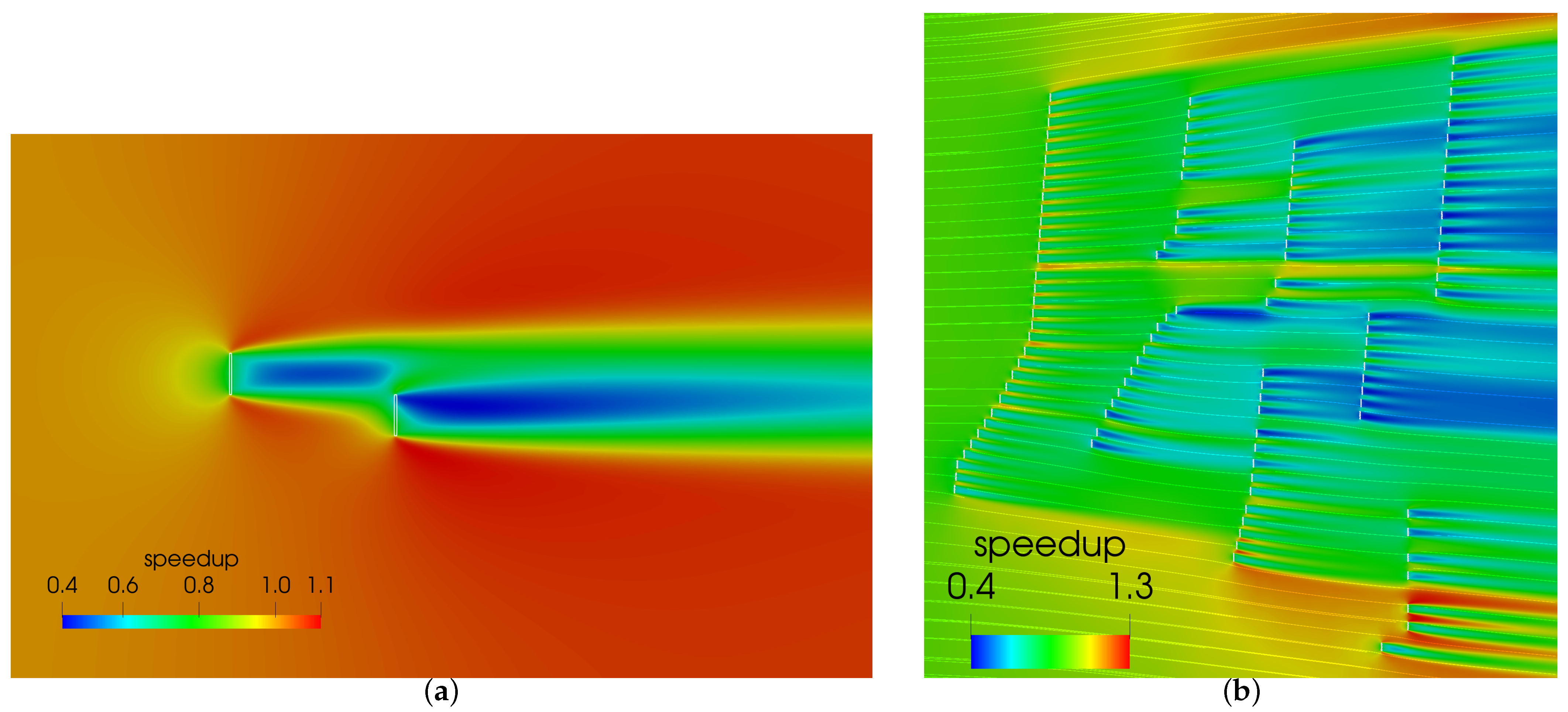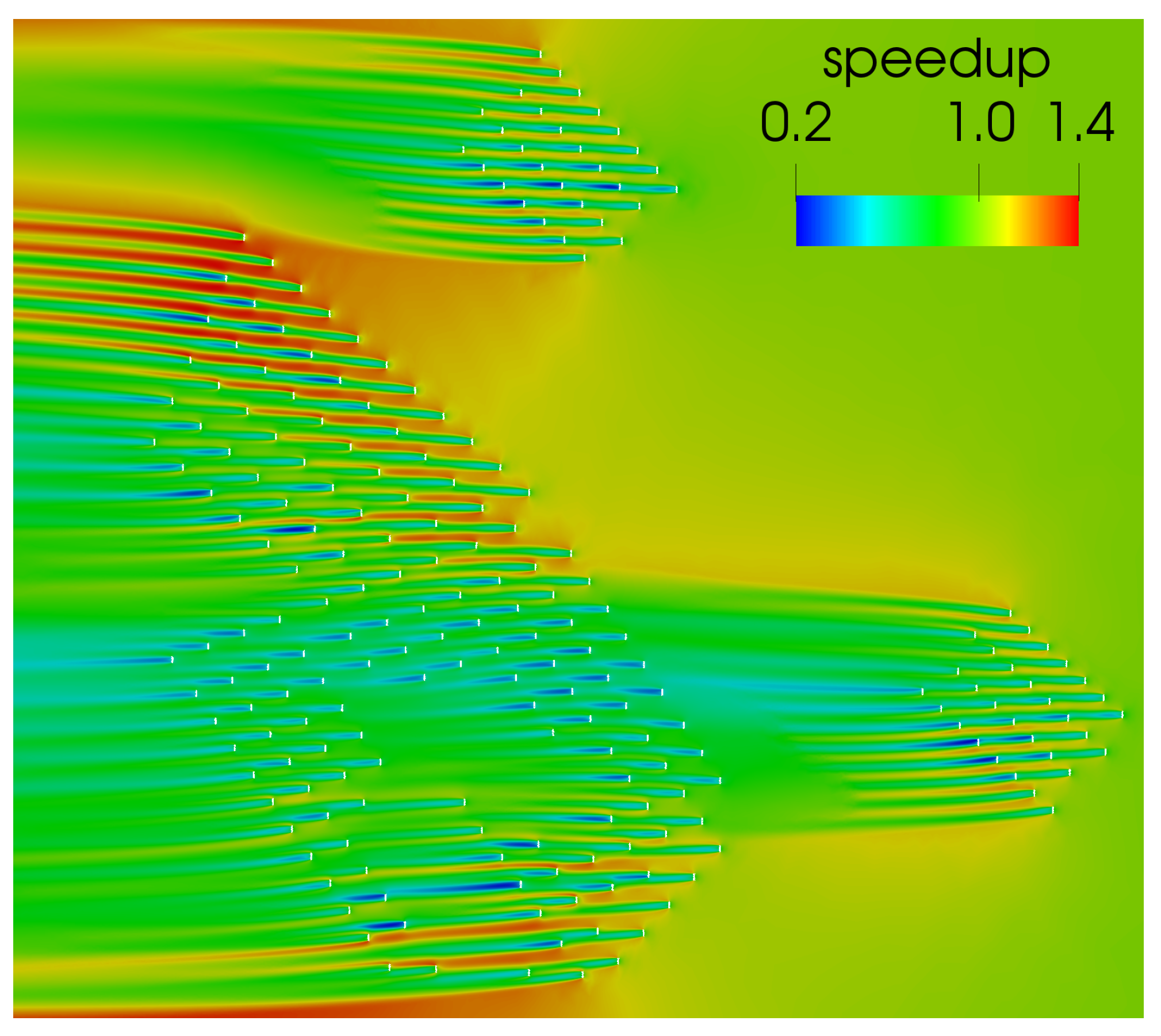Figure 16 illustrates the solution obtained after the adaptive process finalizes.

6.3. Validation of the Turbine Realignment Process

The objective of this example is to validate one of the features of this work: the capacity to realign the turbines according to the flow during the simulation. The misalignment of the turbines is a common issue for complex topographies. As detailed in [46], where different topographic scenarios are simulated, complex topographies produce a close to ground misalignment of up to 45 degrees with respect to the inflow direction. Since this misalignment is due to the interaction between the flow and the orographic features, it can not be known a priori. Thus, the standard pipeline setting the normal of the discs according to the inflow may produce a high deviation with respect to the actual normal. The turbine misalignment is also a common issue for complex wind farm configurations, where upstream turbines produce a perturbation of the wind direction.

To emulate this issue with our 2D test framework and validate the realignment process with a known solution, a misalignment of the turbine with the inflow is enforced—see Figure 17a. The inflow condition is an horizontal flow that moves from left to right (with unitary direction $(1, 0)$), while the disc is oriented with an imposed misalignment of 45 degrees. Next, the realignment adaptive simulation process detailed in Algorithm 3 is applied.

Figure 17 presents three steps of the realignment process. In the final step, the normal is $(-1, 0)$, which is consistent with the inflow condition. This resulting normal validates the realignment procedure. For the current configuration, the normal to the discs should be the inflow direction, since there are no upstream turbines (or orographic features) that alter this direction. For the presented case, four iterations of the correction algorithm are necessary. In total, eleven mesh adaptation steps are performed, featuring meshes from 4000 to 6000 nodes.

6.4. Actuator Disc Realignment in a Wind Farm Featuring 115 Turbines

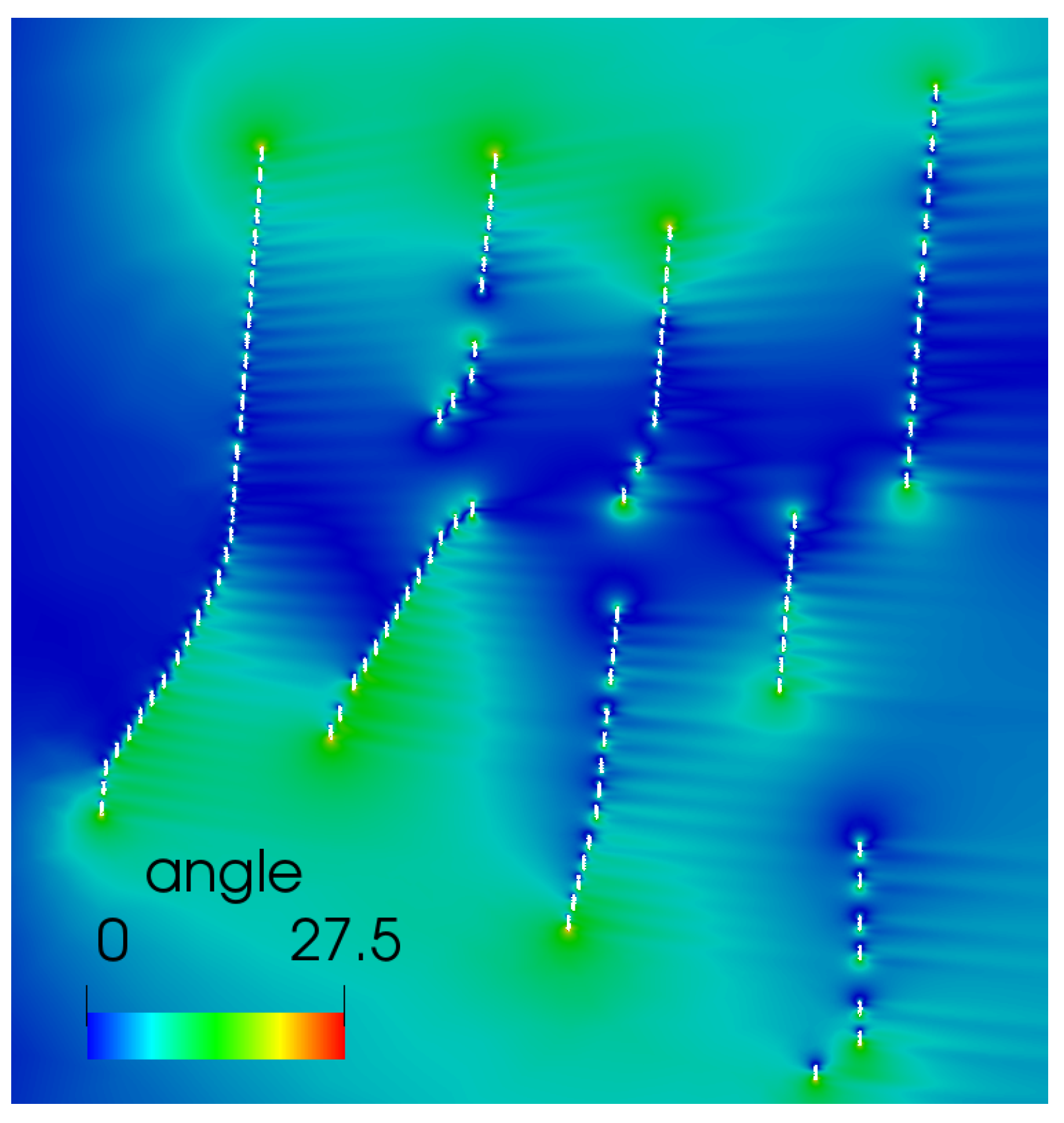
The objective of this section is to illustrate the application of the adaptive simulation process with actuator disc realignment—Algorithm 3—to a section of real wind farm located in Spain featuring 115 turbines. Although the effect of the turbines in the flow is not as large as the one from the topography in onshore scenarios, herein, the realignment algorithm is used to correct the orientation of the turbines according to the effect of upstream turbines.

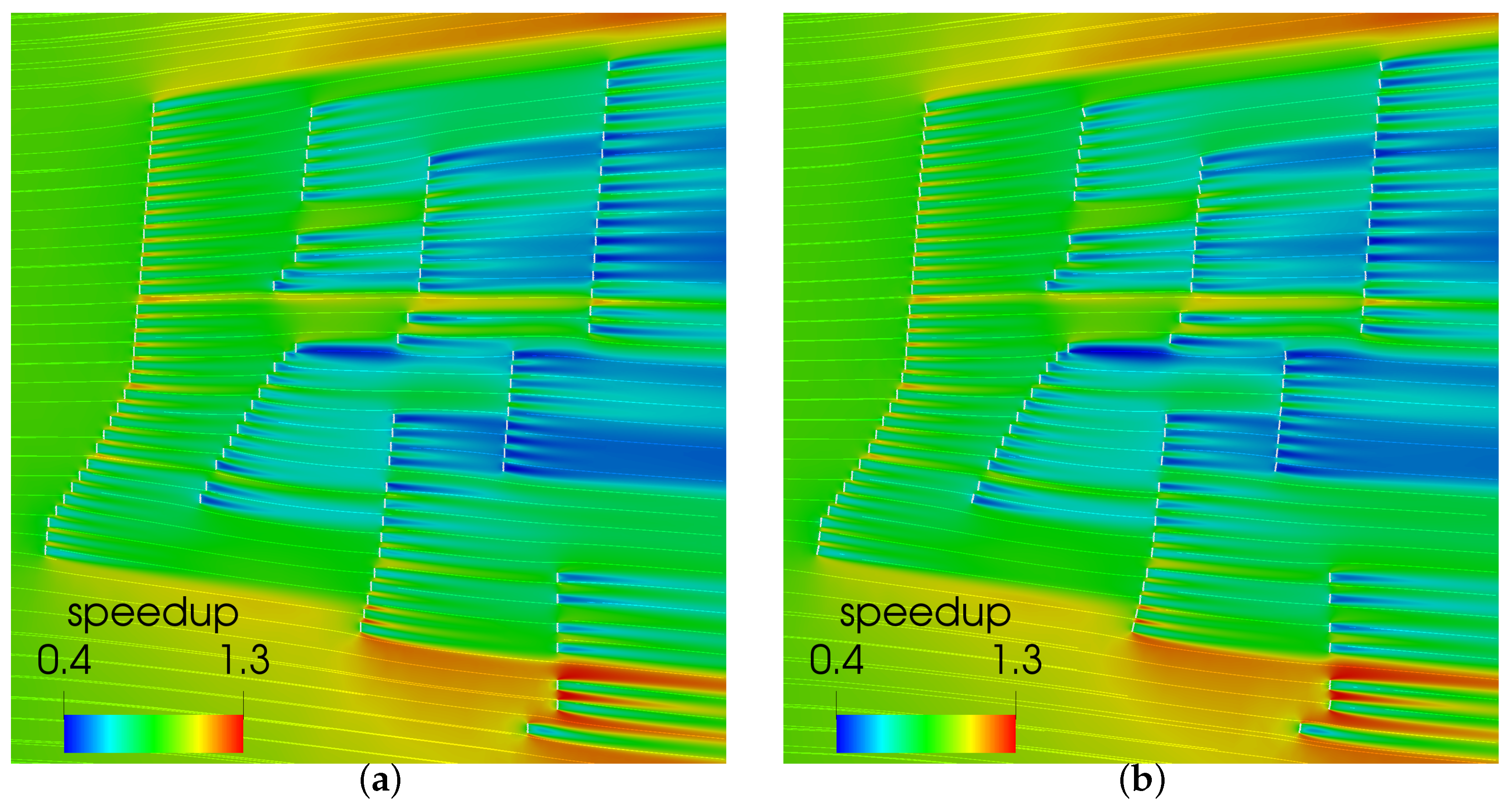
According to Algorithm 3, the actuator disc configuration is set according to the inflow direction, and then the simulation and adaptation cycle is iterated until convergence. The resulting solution is illustrated in Figure 18a. In addition to coloring the mesh with the solution, the streamlines are plot to illustrate the behavior of the flow. Although no topography is present, there is a shift in the wind direction resulting from the effect of the turbines in the flow. Figure 19 shows the angle deviation between the inflow condition and the actual flow configuration on the domain. It can be observed that there is a maximum of 27 degrees of deviation in the flow in all the domain. Restricting this deviation to the actuator disc regions, the maximum deviation of the discs with respect to the actual flow is 14 degrees. Figure 20 shows a closeup to the wind farm regions with higher angle deviation, and consequently, higher turbine realignment. Those turbines, located at the end of each line of turbines, feature corrections of 10 to 14 degrees.

The process concludes after five correction iterations. Since the initial condition is already converged, each correction iteration features only one adaptation step. The number of nodes of the initial adapted mesh oriented according to the inflow condition is 289 K (578 triangles), whereas the final one has 290 K nodes (580 triangles). The turbine with a largest correction features an angle shift of 13.81 degrees with respect to the initial orientation. The final configuration and solution is illustrated in Figure 18b and Figure 20c,d.

It must be highlighted that since the flow is already converged in the first configuration, the solver requires of at most 2–3 iterations to converge to the updated actuator disc configurations (the initial condition is close to the final). That is, once the adaptive process to the first configuration is converged, the correction procedure features a low cost. In particular, for this example, the first adaptive iteration requires the $90\%$ of the cost of the correction process. Thus, for a cost similar to an adaptive simulation process, the turbine realignment procedure achieves a reliable representation of the wind farm configuration. We remark that any other realignment criteria to the normal of the discs could be implemented if desired. The implemented criteria illustrates the potential of the level set representation to couple the simulation with the desired correction process.

7. Conclusions

Herein, a novel wind farm simulation framework is presented, featuring an actuator disc modeling of the turbines. The main features of the framework are that it allows mesh adaptation to the solution and the capacity of aligning the disc models with the flow. These features are attained by means of first representing the actuator disc models as a level set function to be captured by the mesh. Then, the mesh is adapted to capture those level set using the well established technology to perform mesh adaptation with respect to a given metric. To achieve this, simplicial meshes are used, discretizing the actuator discs with the desired mesh size, but not imposing that the mesh matches the actuator disc boundary.

Using the devised metric-based actuator disc discretization enables, in a straight-forward manner, the capacity to adapt to any target solution field. From the solution interest field (herein, velocity magnitude), an additional metric is considered and is intersected with the level set one. Thus, adaptation to both the actuator discs and the flow solution can be performed at once.

The actuator disc level set modeling is validated, testing that it preserves the theoretical convergence rates without a loss of accuracy with respect the standard approaches. In addition, by enabling mesh adaptation to the solution, standard boundary tight approaches are outperformed. The novel approach enables an increase in accuracy, converging to the same solution than boundary tight representations with a reduced cost, and also attaining the theoretical quadratic convergence.

One of the main features of our work is the capability to realign the turbines according to the current flow during the simulation process. In standard wind farm frameworks, the turbine configuration is determined a priori. However, topographic effects and turbine interaction modify the wind inflow, which produces a misalignment of the turbines with the flow. We propose an adaptive procedure capable of redefining the level set field according to the wind flow during the simulation. Then, the derived metric and the mesh adaptation process generate a new mesh that reproduces the updated actuator disc configuration.

Several results that support the novel presented features are presented. The convergence and accuracy of the adaptive simulation process is validated, and then it is applied to a set of four neighboring wind farms composed by 219 turbines. Next, the actuator disc realignment process is validated, and it is applied to simulate a wind farm composed by 115 turbines, correcting the turbine configuration according to the flow during the simulation.

In the near future, we will extend the framework to simulate 3D wind farm configurations featuring complex topographic scenarios and modeling the Coriolis effect. The proposed framework will be introduced in our 3D CFD model [1,2] and implemented in the parallel multi-physics solver Alya [50,51]. The extension of the approach for full 3D configuration steps by generating an initial tetrahedral mesh conformal with the topography, and then adapting the mesh to the interface metric. The two major steps are, first, the metric evaluation, which demands computing the distance to the actuator discs, and then computing the Hessian of the function to define the corresponding metric. The second step is developing a 3D adaptation framework coupled with our solved, which is currently under development.

The proposed framework can be implemented in any given CFD program that features mesh adaptation. Mesh adaptation is the key to remove the actuator disc modeling from the preprocessing step, automatizing it during the adaptation step to the solution and simultaneously enabling the realignment with the simulated flow. In particular, in this work, we have developed an specific purpose solver to test the concept and study the potential advantages, but as just detailed, we aim to incorporate it to the parallel solver Alya. One can implement the proposed approach in any given CFD program (such as Ansys, Simcenter or OpenFOAM) steps by defining the interface function, and incorporate the derived metric in the solution-driven adaptation of the target solver.