Abstract
PV systems are a popular energy resource, prevalent worldwide; however, shade faults manifested in PV systems limit its power conversion efficiency. The occurrence of multiple power peaks and their location are highly uncertain in PV systems; this necessitates the use of complex maximum power point tracking algorithms to introduce high voltage oscillations. To address this issue, a new reconfigurable PV array to produce a global maximum power point (GMPP) algorithm close to the Voc regions was introduced. This enables the use of a simple Perturb and Observe (P&O) algorithm to easily track GMPP. For reconfiguration, a simple 5 × 5 PV array is considered, and a new physical relocation procedure based on the position square method is proposed. Performance of the proposed reconfiguration model is tested for four various shade events and its row current evaluations are comprehensively analyzed. Furthermore, evaluations of fill factor, mismatch loss, and power loss are quantitatively compared against Dominance Square and TCT schemes. Since the power enhancement is ensured in a reconfigurable PV array, the fixed reconfiguration is tailored to suit residential PV and microgrid systems. For MPP evaluations, hardware demonstrations are performed with a lab scale prototype model developed with a PV simulator and a DC–DC power electronic interface. The I–V characteristics of conventional and reconfigured models are programmed into the simulator and the use of the hill climbing algorithm is validated. To analyze the voltage and power oscillations with MPP tracking, the PSO algorithm is also tested for two test patterns and its results are comprehensively studied.
1. Introduction
Minimizing the possession of carbon footprints, solar energy has emerged as a strong competitor in the global electrical market [1]. Particularly, the diligence of PV in constructing micro- and nano-grids is a strong incentive to establish PV as an alternative to conventional power generation [2]. However, shade faults manifested by environmental impacts have raised concerns over its continuous and efficient power generation.
As an outcome of shade events, dissimilar row currents are encountered that induce mismatch loss in PV arrays. Hence, PV reconfiguration at the design stage is performed on Total Cross Tied (TCT) interconnections to diminish the severity of the shade effect [3]. Note that TCT is one of the interconnection schemes in PV arrays that produce a reduced mismatch and power loss. Reconfiguration in general reiterates the current–voltage characteristics to reduce the row current difference, thereby multiple power peaks are reduced [1]. Extensive research in the literature on PV array reconfiguration is found, and it is categorized by either of the following: (i) Physical Array Reconfiguration (PAR) and (ii) Electrical Array Reconfiguration (EAR). The former uses simple rewiring to interconnect the PV modules whereas the latter use power electronic devices, manual switches, and controllers to reconnect the PV array. PAR methods are puzzle-based reconfiguration techniques, which are performed once on the PV array. Methods like SuDoKu [4], Futoshiki [5], Zig-Zag [6], Dominance Square [7], and two-phase methods [8] are predominantly popular for applications in PV arrays. Though PAR has lengthy interconnection wires, it is considered as a promising solution to reduce the shade effects in large PV arrays. In the case of EAR, the reconfiguration is performed only when the shade event is diagnosed [3]. Furthermore, EAR schemes have undergone a huge transformation since their inception, where the reconfiguration via EAR is made with manual switches and relays [9,10]. However, with the recent inclinations and developments in semiconductor devices, EAR faces more competition in becoming an economical alternative for PAR schemes. However, EAR schemes process repeated switching to arrive at an optimal switching matrix; a shade pattern that can produce narrow row current difference. This leads to semiconductor switch degradation accompanied by unknown manual errors. However, the advent of optimization techniques has resolved the aforementioned problem with multiple switching and results in a switching matrix with narrow row current difference [11,12]. Nevertheless, EAR techniques need sensor data, controller, and processor arrangement to program the optimization. Overall, in comparison with PAR, EAR is found to be a non-economical and complex solution for current application in PV arrays.
On the other hand, despite the design stage reconfiguration, PV arrays demand maximum power point tracking controllers to operate the PV array at maximum power point (MPP) [13,14]. In the literature, many MPP techniques like hill climbing, incremental conductance, optimization methods, and hybrid approaches are proposed [15,16,17]. It is noteworthy to mention here that despite the reconfiguration strategies and types of shade event, MPP trackers are mandatory in a PV system to operate PV array at the global maximum power point (GMPP). Among many others, the most favored MPP algorithms deployed currently are the Perturb and Observe (P&O) and hill climbing methods. However, Perturb and Observe (P&O) MPP trackers may not always guarantee their operation at GMPP during a shade event. This is because of two uncertain reasons: (i) improper duty cycle initialization and (ii) the existence of multiple power peaks during the event. Besides this, a value of GMPP that differs from the open-circuit voltage (Voc) is a major setback in tracking the precise GMPP. Therefore, there exists a gap between the PV system design and the deployment of maximum power point tracking. In addition, it is necessary to envisage an appropriate reconfiguration strategy to suit the P&O MPP tracking.
Thus, in this research, a novel method with a blend of reconfiguration and MPP tracking is investigated to obtain the maximum benefit from the environmental conditions. After analyzing the literature, we propose a novel sum of position square; a physical relocation scheme for the system. Furthermore, utilizing the basics in fundamental mathematics, the positions of individual PV panels are reconfigured by squaring their current position in the PV array. For a better understanding, a set of rules is exclusively prescribed to attain the final dispersed matrix. In addition, a column-wise relocation process helps the proposed method to follow a unique shade dispersion process that can avoid laborious interconnections, unlike conventional physical relocation schemes. Meanwhile, the reconfiguration performed in Total Cross Ties (TCT) interconnection is always ensured to produce a global power peak closer to Voc. This ensures duty cycle declaration closer to Voc (0.1 duty) that will always guarantee GMPP operation. Furthermore, this arrangement eradicates the need for heuristic-based MPP tracking, avoiding complex computations. The proposed method is tested with a 5 × 5 PV structure since the research presents a solution to mitigate shade difficulties occurring in micro- and nano-grids. Furthermore, it is also a promising solution for deployment in residential PV systems. For evaluations, four various test cases such as (i) Short Narrow (SN), (ii) Short Narrow (SN), (iii) Long Wide (LW), and (iv) Long Narrow (LN) are considered and the results are visualized using the simulated I–V and P–V characteristics. Simulations are performed in a MATLAB/Simulink environment and the case studies with HC MPP tracking are presented. Additionally, the results of the TCT and Dominance Square (DS) interconnection schemes are also given to contribute to a fair, comparative study. Performance indices such as (i) fill factor, (ii) mismatch loss, (iii) power loss, and (iv) capacity utilization factor are meticulously calculated to gauge the efficacy of the proposed PV reconfiguration strategy. The major contributions of the proposed work are:
- ▪
- A new physical relocation procedure for a simple 5 × 5 PV array is proposed for micro- and nano-grid applications.
- ▪
- For any shade event, the occurrence of GMPP is always ensured to be closer to the Voc.
- ▪
- A blend of reconfiguration and maximum power point tracking is proposed for the first time.
- ▪
- Despite the type of shade and GMPP location, a simple hill climbing (HC) MPP tracking is proven to track GMPP.
- ▪
- A new two-phase tracking scheme is introduced in the HC method for the first time, where GMPP location identification is possible within five to seven samples.
2. PV Modelling for Reconfiguration Process
Photovoltaic design structures conventionally use series–parallel architecture to connect PV arrays. However, to handle shade phenomena, various array structures are studied in the literature. In this work, TCT-based reconfiguration is preferred. Furthermore, the modelling of a TCT interconnection, row current calculation and an overview of array reconfiguration is presented in this section.
2.1. Modeling of Total Cross Tied (TCT) Interconnection
TCT interconnection in PV arrays is an extracted version from conventional series–parallel interconnections, where every row of the PV array is cross-tied to formulate Total Cross Tied (TCT) interconnections. Cross-ties in TCT interconnections double the life span to increase the power output. In TCT array structures, circulating current loops are formed and encounter the following effects: (i) circuital voltage limitations are notably observed and (ii) differential current flow between PV modules of the same string is seen.
Partial shade conditions (PSC) are one of the most common effects in PV arrays and hence, it is important to analyze the row current evaluations in TCT interconnections. This enables the PV interconnection to accurately predict the location of global peak (GP) power. To understand the row current calculation, a simple m × n PV array is considered and the expressions for row current of a TCT interconnection is explained as follows. The output current of an ‘m’ row is calculated as the sum of the individual current limits of the PV panels and its calculation with TCT interconnections is given as follows.
where ‘’ is the module current limit at full irradiance, (), and where is the irradiation level (n = column index). Applying Kirchhoff’s Voltage Law for a m × n PV array, the voltage of a PV array with TCT interconnections is given as
where, ‘’ is the array voltage and maximum array voltage at the ‘ith’ row, respectively. The current at each node in the array is estimated by applying Kirchhoff’s Current Law (KCL) and the total array current is given by
2.2. Row Current Calculation—TCT Interconnection
Row current calculation in TCT interconnected PV arrays requires a fundamental understanding of the row current estimation. Since cross-ties exist in TCTs, the shade dispersion research investigations add invaluable knowledge to array reconfiguration. The proposed reconfiguration is performed on a simple 5 × 5 PV array and the basic formula to estimate the row current is given in Equation (4)
where ‘’ is to the ‘nth’ row current, ‘’ is the module irradiation, ‘’ is the irradaitionat Standard Test Conditions (STC), and ‘’ is the module current.
2.3. Array Reconfiguration—An Overview
Array reconfiguration is just a circuital reassembly of PV interconnections to mitigate the shade faults in the PV array. Technically, reconfiguration narrows down the difference in row current that appears during the shade event. To exemplify the effect of row current and its immediate cause, a simple short wide shade event is demonstrated with a 5 × 5 PV array as follows. For explanation, a TCT interconnected PV array is presented in Figure 1a. From the figure, it can be seen that the last two rows of the PV array alone are shaded; therefore, three different row currents are seen (4.5 A, 3.0 A, and 1.0 A). The detailed row current calculation performed on the PV array is presented in Equations (5)–(7).
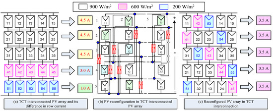
Figure 1.
Reconfiguration process in PV array.
From the row current values, a large row current difference is obvious; hence, PV characteristics become extremely complex. Mathematical formulations and explanations of row current can be found in detail in [8,18]. To reduce the effect of shade, the reconfiguration of TCT interconnections is performed, as shown in Figure 1b. Note that the reconfiguration is made only once, and it remains unaltered for any further change in shade. As a result of the location changes, a new shade pattern with a unique row current is attained, as shown in Figure 1c. The row current calculation for the reconfigured arrangement is given in Equation (8).
Owing to the row–current calculations, the necessity for PV reconfiguration is found to have a major impact in the PV design stage. Advantages of the existence of reconfigurable PV arrays are given as follows: (i) shade faults can be mitigated (ii) PV arrays with narrow row current differences can be obtained, and (iii) the size of installed capacity can be altered based on consumer demand.
3. Position Square Reconfiguration Scheme for 5 × 5 PV Array
Circuital reassembly of a 5 × 5 PV array to suit micro- and nano-grids is explained in this section. Reconfiguration in this research is implemented on a 5 × 5 PV array as it is one of the optimal PV patterns for residential and MicroGrid applications. However, the proposed procedure can suit any PV array irrespective of its structure. Reconfiguration of the proposed method is made by just squaring its current position. For a detailed understanding of the method, the position of any PV panel is hereby indicated as ‘ij’, where ‘i’ denotes the row number and ‘j’ denotes the column number. Detailed panel positions and their relation to ‘ij’ can be understood from the 5 × 5 PV array presented in Figure 2a. Note that the proposed method follows only the column-wise reconfiguration to ease the rewiring complexity. The reconfiguration process of the proposed sum of position square method is explained in the following. In the initial step, the sum of the position of each panel is mathematically squared as (i + j)2. The proposed method undergoes reconfiguration only based on the resultant squared value. In brief, only the first column elements in the PV array are squared, as shown in Figure 2b. It is important to note here that if the squared value is double-digit, then sequential addition of the resultant value is performed until a single-digit value is obtained. A typical example of this can be seen in Figure 2b with elements ‘31’, ‘41’, and ‘51’ in the first column of the 5 × 5 PV array.
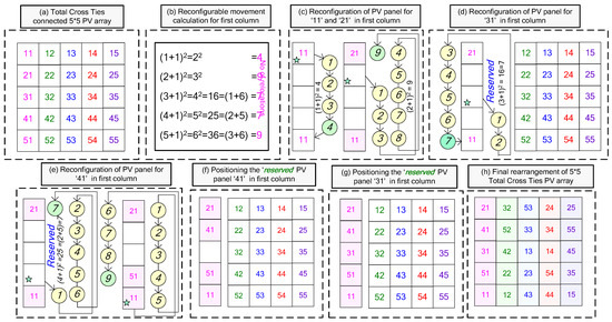
Figure 2.
Reconfiguration process with position square method—Application to 5 × 5 PV array.
As the proposed method undergoes relocations based on square values, it becomes important to explain the relocation movements with the method. Hence, the reconfiguration of first column elements in the PV array is explained as follows. To explain, the mathematical sum of PV panel ‘11’ is squared as shown in Figure 2c. As the method is framed to follow a column-wise relocation procedure, the PV panel at position ‘11’ is moved four positions downward and relocated to position ‘51’. Similarly, PV panel position ‘21’ is relocated nine places to ‘11’. During reconfiguration, if any of the PV panels are already occupied, then the corresponding PV panel is reserved for later relocation. To represent the reserved relocation process, the PV panels bearing position ‘31’ and ‘41’ with reserved status are shown in Figure 2d,e, respectively. Furthermore, the reconfiguration of PV panel ‘51’ in the first column is also shown in Figure 2e.
As three panels, ‘11’, ‘21’, and ‘51’, occupied the reconfigurable places, the reserved panels ‘41’ and ‘31’ are made to occupy the empty places of the first column in descending order. Reconfiguration of reserved PV panels ‘41’ and ‘31’ can be seen in Figure 2f,g, respectively. Following the procedure of the sum of the position square, the remaining columns in the 5 × 5 PV array are reconfigured, as shown in Figure 2h. Reconfiguration rules of the proposed method are given in the following.
- Rule 1: Perform the sum of position square for all the elements in the PV array following the mathematical expression (i + j)2. The resultant value gives the movement for the respective PV panel undergoing reconfiguration.
- Rule 2: If the resultant value holds a two-digit value, perform sequential addition until a singular digit is obtained.
- Rule 3: Rearrange/rewire the PV panels based on the sum of position square value (column-wise relocation).
- Rule 4: If any of the PV positions in a respective column are already occupied, ‘reserve’ the PV panel for later reconfiguration.
- Rule 5: When all the PV panels in a respective column are reconfigured, place the reserved PV panels in descending order of position value (this is also termed as reverse chronological order).
4. Simulation Results and Discussion
To test the anticipated reconfiguration method, four various shade cases were considered. Note that these test cases were carefully considered as they are prone to occur in the real world. In addition, these shade cases have been studied extensively in [14,15] the literature, which justifies the selection of the shade patterns. For simulations, MATLAB Simulink installed on a personal computer with 16 GB RAM and an i7 processor was used. For fair validations, the results of the proposed methods were quantitatively compared with the Dominance Square (DS) method and the TCT method. For fair validations, the PV panel details used for simulations were the same as used in the DS method. Furthermore, theoretical and simulation validations are tabulated to show the success of the shade dispersing ability with the proposed method. The success of shade dispersion was gauged based on (i) the number of power peaks in P–V characteristics and (ii) the appearance of global power peak close to Voc. In addition, the row current difference minimization and its effect on shade dispersion were analyzed with a 3D case study.
4.1. Simulation and Validations—Patterns 1 & 2
The short, wide shade case, pattern 1, is prone to occur in reality very often. Thus, observations on this shade case have major significance in recommendation of the proposed scheme for real world implementation. For experimental investigations on this shade case, three various irradiations were considered (900 W/m2, 200 W/m2, and 600 W/m2). The shade pattern of TCT and the proposed scheme is shown in Figure 3a,b. From the dispersed shade pattern, it was observed that only three current changes with negligible difference were produced. As a consequence, the proposed method has produced a maximum power of 1413.43 W, close to the Voc. For comparison, the TCT and dominance square method was also simulated and its power values were also benchmarked as 1096.72 W and 1385.05 W, respectively. After analysis, it was perceived that the proposed method and the DS method have obtained global power close to Voc; however, the shade dispersion ability with the proposed scheme is maintained at a high level. The I–V and P–V characteristics of pattern 1 are shown in Figure 3c,d, respectively.
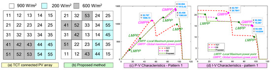
Figure 3.
Shade pattern 1: (a) TCT arrangement, (b) Proposed arrangement, (c) P–V characteristics, (d) I–V characteristics.
For shade pattern 2, a simple short, narrow shade pattern is considered. Similar to shade pattern 1, three various irradiations were considered (900 W/m2, 500 W/m2, and 600 W/m2). In this shade case, only four panels were shaded in the 5 × 5 PV array. In the shade pattern for TCT, the rightmost corner is shaded, as shown in Figure 4a. In the TCT shade case, only two current changes are seen, whereas the proposed shade dispersion pattern has three row current changes with a negligible difference. A graphical representation of the dispersed 5 × 5 PV array is shown in Figure 4b. Acknowledging the row current changes with TCT and the proposed method, the I–V and P–V characteristics are plotted in Figure 4c,d, respectively, producing a global power of 1661.33 W and 1755.3 W. Despite the DS model producing global power (1691 W) closer to Voc, the proposed scheme has obtained a higher power, showing the potential of the proposed method.
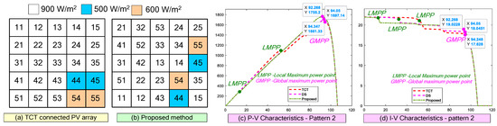
Figure 4.
Shade pattern 2: (a) TCT arrangement, (b) Proposed arrangement, (c) P–V characteristics, (d) I–V characteristics.
4.2. Simulation and Validations—Patterns 3 & 4
The long, narrow shade pattern is one of the eventual patterns that occurs in reality. Furthermore, the shading phenomenon in this case always guarantees the occurrence of a power peak to the right of Voc. However, it is important to maximize the available power via reconfiguration. Thus, a simple long, narrow shade pattern with three irradiation values was programmed into TCT, as shown in Figure 5a. Furthermore, the dispersed shade pattern for the proposed scheme is presented in Figure 5b. Acknowledging the nature of the shade case, the TCT, DS, and the sum of position square methods have produced global power peaks close to Voc. However, the proposed method has a better dispersion, obtaining a maximum power of 1629.19 W compared to the DS (1599.3 W) and TCT (1422.8 W) methods. Despite there being less scope to maximize the power, the proposed method has increased the maximum power by 200 W compared to TCT and 30 W compared to DS. In addition, the reconfigurable wiring complexity is also reduced in the proposed scheme. A detailed view the simulated results of TCT, DS, and the proposed scheme is presented in Figure 5c,d, respectively.
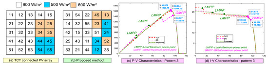
Figure 5.
Shade pattern 3—(a) TCT arrangement, (b) Proposed arrangement, (c) P–V characteristics, (d) I–V characteristics.
A non-conventional shade pattern, shade pattern 4 would be considered quite unusual if it were to happen in reality. In this shade case, the five farthest left PV panels are shaded in the last three columns. Surprisingly, the global power values of the proposed and DS methods are the same, at 1634.28 W; however, TCT only produced 1422.93 W. A representation of the shade profile of TCT and the proposed scheme are shown in Figure 6a,b. In addition, the simulated I–V and P–V characteristics of DS, TCT, and the sum of position square methods are presented in Figure 6c,d, respectively.
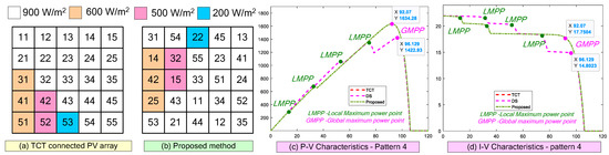
Figure 6.
Shade pattern 3: (a) TCT arrangement, (b) Proposed arrangement, (c) P–V characteristics, (d) I–V characteristics.
4.3. Theoretical Calculation—Shade Patterns 1–4
To verify the simulated findings theoretically, values of voltage, current, and power values were mathematically calculated and are tabulated in Table 1. Note that ‘Vm’ and ‘Im’ denote the maximum voltage and maximum current value of the PV panel, respectively. From the table, it can be seen that the TCT method has failed to produce global power close to Voc (5 Vm) in shade patterns 1 and 3. Furthermore, the observation that the DS and sum position square methods always guarantee to produce a global maximum at 5 Vm is notable. However, in all the shade patterns the power coefficient of the proposed method is always higher compared to the DS method. Although the simulations of DS and sum of position square methods have given the same value of global power for pattern 4, the theoretical power coefficients are found to be different. More importantly, the bypasses are found to be low with the proposed scheme with a higher theoretical power coefficient.

Table 1.
Theoretical row current calculation for shade patterns 1–4.
4.4. Row Current Evaluations—3D Study
To identify the success of shade dispersion ability with the proposed scheme, a 3D representation of row current values corresponding to row and column numbers of shade patterns 1–4 is presented in Figure 7. For understanding, the maximum and minimum current produced by TCT and the sum of position square methods are also marked. Furthermore, the measure of success with shade dispersion can be determined in the following way: a more linear current curve indicates a lower row current difference and therefore a high shade dispersion ability. We highlight the fact that, in all shade cases, the proposed method always guarantees a higher shade dispersion ability relative to TCT interconnection. Thus, the proposed method has all possibility to emerge as a promising solution for conventional TCT.
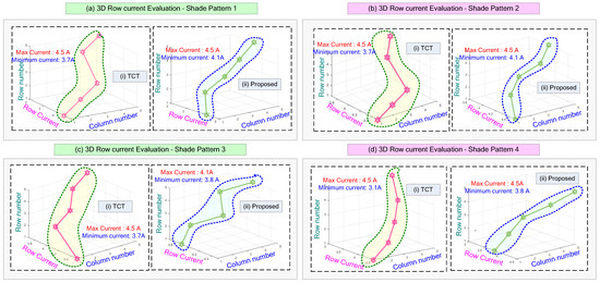
Figure 7.
3D row current evaluation for TCT and the proposed method forshade patterns (1–4).
4.5. Performance Parameters—A Case Study
Performance parameters are one of the major metrics in array reconfiguration for gauging the success rate. For this analysis, performance parameters like Fill Factor (FF), Mismatch Loss (ML), and Power Loss (PL) are considered. Mathematical expressions to evaluate the method performance are given as follows:
where ‘’ is the global maximum power point (GMPP) at STC (Standard Test Conditions), ‘’ is the GMPP in the partial shade case, and ‘’ is the global maximum power of a shade pattern. On valuation of the aforementioned performance parameters, a quantitative table indicating ML, FF, and PL is given in Table 2. Furthermore, a graphical bar chart representation has been plotted, as shown in Figure 8, To visualize the performance indices. From the table, the following conclusions are drawn:
Table 2.
Performance parameter calculation for TCT, DS and the sum of position square methods.
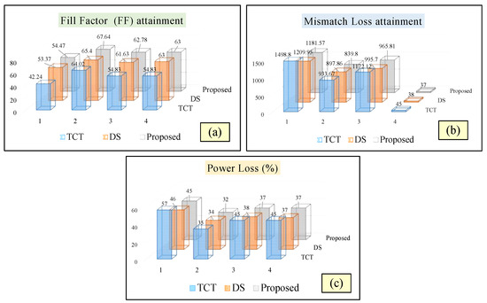
Figure 8.
Graphical representation of TCT, DS and the proposed scheme for (a) Fill Factor attainment (b) Mismatch Loss, and (c) Power Loss (%).
- Fill factor attainment with the sum of position square method is always 5% higher compared to TCT and 2% higher compared to the DS method (except in shade pattern 4).
- As mismatch loss indicates the power loss, a lower mismatch loss gives a higher maximum power extraction. Thus, the proposed method always guarantees a lower mismatch and power loss, establishing its success quantitatively.
- The ML and PL of shade pattern 4 for the DS method and the proposed scheme are the same since they share the same global power value.
According to this wide comparative study, the proposed sum of position square method has shown a superior performance relative to the TCT and DS configurations. Thus, the proposed reconfigured PV model has assured the possibility of producing a global power peak close to Voc; hence, it is highly recommended to replace the SP configuration for MPP tracking.
4.6. Qualitative Comparitive Study
To demonstrate the suitability of the sum of position square scheme for MPP tracking, various parameters have been considered qualitatively and are presented as a wheel chart in Figure 9. For comparison, EAR, TCT, DS, and proposed schemes are comprehensively gauged for all the four shade patterns discussed in Section 4. Various parameters considered in the study are: A-sensor requirement, B-ability to produce row current, C-procedural complexity, D-rewiring complexity, E-mismatch loss, and F-multiple power peaks in P–V characteristics. The aforementioned parameters are gauged at a level from low to high and it can be understood in the following way: the method closer to the inner diameter of the wheel is considered to be more promising for MPP implementation, and the method with the larger diameter has higher limitations and is least recommended for PV arrays.
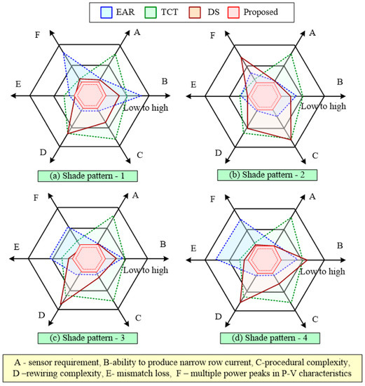
Figure 9.
Wheel chart representation of various performance indices for shade patterns (1–4).
Considering the plotted results of the wheel chart in Figure 9, the proposed method always ensures that optimal performance is delivered for all shade patterns. More importantly, the consistency of the proposed reconfigured scheme in having limited power peaks is the most important factor for the reconfiguration method. In addition, values of the mismatch loss and procedural complexity parameters are always found to be in the low range for the proposed scheme, and also gives a less complex PV array configuration. On the other hand, the EAR method records a higher range, adding to its limitations. Overall, the proposed position square method has a greater ability to produce GMPP close to the Voc with reduced complexity, and this is most beneficial for MPP implementation.
5. Design of Maximum Power Point Tracking for Reconfigurable PV Micro Grid Systems
Maximum power point tracking is an integral part of the power conversion system to achieve maximum conversion. Particularly, PV systems under different shade patterns demand MPPT controllers to distinguish the local maxima. However, in this work, a new two-point MPP tracker via the hill climbing method is proposed for reconfigurable PV arrays. It is important to note here that the sum of the position square method is always ensured to have a global maximum close to the Voc. Hence, duty declaration close to the Voc (0.1 duty) always ensures a smoother tracking of the Global Maximum Power Point (GMPP). Furthermore, to reduce the needless delay in tracking, a stepwise mathematical tracking in change in duty () is introduced here for the first time. The coherent idea behind the methodology is to follow a higher step size until the GMPP vicinity is reached (exploration), and vice versa, to exploit the GMPP accurately. This enables the proposed method to follow two step sizes in which certainly avoids initial power oscillations and voltage fluctuations in the power electronic interface. As the proposed method is implemented on a 5 × 5 PV array, the proposed tracking strategy is tailored to suit all residential and microgrid applications. A detailed explanation of the methodology and its hardware implementation is discussed further.
5.1. Two-Step Hill Climbing Method for Reconfigurable PV Arrays
The hill climbing method is just a perturbation in duty cycle () and its periodic reversal in mathematical sign to operate at MPP in P–V characteristics. However, this method utterly fails to track MPP under shade cases. Meanwhile, it is noteworthy to mention here that reconfiguration strategies guarantee their global power peak occurrence close to the Voc. Thus, duty cycle initialization close to the Voc will enable HC to be accurately implemented for GMPP. Therefore, it is obvious that the HC method alone is capable of operating a PV array at GMPP when a PV array is reconfigured. In order to increase tracking speed, a novel two-step tracking method to follow two step sizes in the change in duty is followed. For the reconfigured PV array, the duty cycle 0.1 is initialized in the constant voltage region. Soon after initialization, the change in duty is updated with a higher step size (10%) until the MPP vicinity is reached. This can be seen in Figure 10. The duty cycle is constantly updated from 0.1 to 0.5. The mathematical formulation used for duty cycle declaration is given in Equation (12).
where ‘’ is the instantaneous power, ‘’ is the iteration number, and ‘’ is the duty cycle. Once, the sign is reversed, i.e., , then the duty cycle is declared as an average of . The mathematical formulation for duty cycle declaration is given in Equation (13).
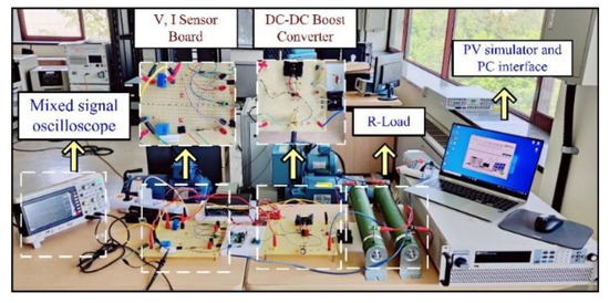
Figure 10.
Hardware prototype model.
After duty cycle declaration, conventional HC-MPP tracking is enabled with a such as 2%.
5.2. Hardware Results and Experimentation
To demonstrate the two-phase HC method, an exclusive hardware prototype model has been developed in the energy systems laboratory at Pohang University of Science and Technology, and is shown in Figure 10. For the hardware testbed set-up, an ETS Terra SAS PV simulator was interfaced with a power electronic interface (DC–DC boost converter), where the duty of the interface was constantly regulated to operate at MPP. In addition, LEM sensors LA25P and LV55P were used at the PV side to read the analog values of voltage and current. Consequently, these analog values of V and I were processed by the Arduino controller to generate a duty cycle for the power electronic interface. To isolate the switch, a driver circuit made by Infineon (EVAL-1ED44176N01F) was utilized. Since the hardware testing model is designed only for 1 KW PV systems, the PV panel model shell 36 Watts was used. The datasheet of shell S36 W PV panel can be found in [19]. Note that for simulations, a 100 Watts PV panel was used.
The hardware specification of the DC–DC converter is given as follows: (i) a switching frequency of 10 kHz, (ii) an inductor value of 1 mH, (iii) a capacitance of 650 V, 100 µF, and (iv) a standalone ‘R’ load of 100 Ω, 15 A. For the evaluations, the shade patterns 1 and 2 presented in Figure 3 and Figure 4 were utilized here and the power voltage characteristics were programmed to the PV simulator. To evaluate the performance of MPP tracking modules, the power values benchmarked in the simulation (100 W) and hardware prototype model (S36) are presented in Table 3. Since the primary objective of this research is to facilitate P&O/HC maximum power point tracking for a reconfigured PV array, the reconfigured PV array characteristics were tested with P&O MPP tracking and the conventional TCT characteristics were tested with the particle swarm optimization algorithm. The detailed observations of voltage, current, and the power values tracked by P&O and PSO methods are comprehensively analyzed in this section. Various parameters tuned for PSO and proposed two-phase P&O method are presented in Table 3. Note that the PSO method is declared with five samples and the convergence to MPP regions are comprehensively attained. The variables tuned for the PSO and P&O algorithms are presented in Table 4.
Table 3.
Voltage, current, and power values for pattern 1 and pattern 2 in simulation and hardware models.
Table 4.
Parameters of PSO, P&O, and the two-phase P&O method.
Having input the reconfigured PV array characteristics to the PV simulator, the two-stage HC algorithm is implemented in the MPP controller to track the MPP. The hardware realization of the MPP tracking applied to the reconfigured PV array is presented in Figure 11. For the hardware realization, two PV patterns (shade patterns 1 and 2) were considered, and the MPP tacking is realized at an interval of 50 s. From the real-time hardware observation, it is confirmed that MPP tracking with the reconfigured PV array has fewer oscillations and the power convergence to GMPP is fast. Following the simulation theory, the HC method is initialized at 10% duty and this method is only applicable for reconfigurable PV arrays. In addition, the appearance of triple point behavior in the HC method convergence justifies the proposed two-phase HC scheme. For shade pattern 2, the two-stage HC method attained 803 W (91 V, 8.7 A) and for shade pattern 1, 754 W (92 V, 8.1 A) was recorded. Furthermore, it is notable that the proposed method took less than five samples to reach the vicinity of GMPP.
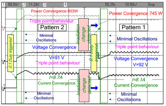
Figure 11.
Hardware experimentation of the two-phase HC method.
On the other hand, the experimental results of PSO are presented in Figure 12. In contrast to the two-stage HC method, the conventional TCT programmed PSO tracking has recorded a poor performance in MPP tracking. In addition, the PSO method has higher power oscillations and a delayed convergence compared to the two-phase HC method. The MPP tracking of the PSO method recorded a power value of 755 W for pattern 2 and 499.5 W for pattern 1. For the PSO code, the parameters are tuned by referring to [19]. Thus, on performance evaluation, it is confirmed that the two-phase HC method is effective in operating at GMPP for reconfigured PV arrays.
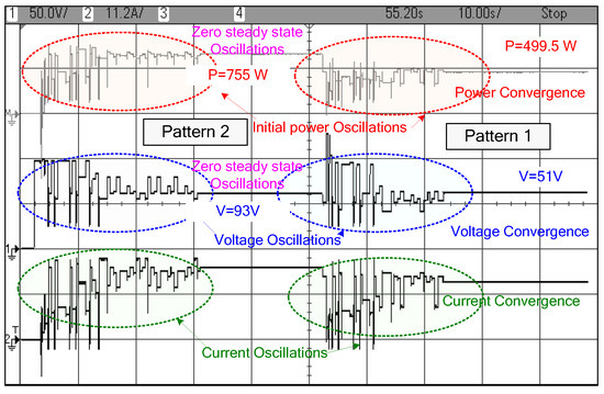
Figure 12.
Hardware experimentation of the PSO method.
6. Conclusions
In this research, a new physical reconfiguration method that always guarantees a global power peak close to Voc is proposed. In addition, a novel fast-tracking hill climbing algorithm is proposed for the reconfigurable PV array. More importantly, HC has been proved to track GMPP for the reconfigured PV array by initializing at 10% duty. A detailed summary of the proposed research is given in the following:
- The proposed reconfiguration method produces reduced mismatch losses compared to the TCT and dominance square methods. Furthermore, the proposed sum of the position square method has demonstrated 10% higher fill factor attainment compared to the TCT method.
- In hardware testing, 98% MPP tracking efficiency is recorded in all test cases with the proposed two-phase HC method.
- Power convergence in hardware for a change in irradiation conditions validates the deployment of MPP tracking in PV systems. In addition, the blend of reconfiguration systems with MPP tracking is a valuable framework for practicing researchers to apply array reconfiguration for MPP tracking systems.
Author Contributions
J.P.R.—Conceptualization, Data Curation, methodology and writing—original draft preparation; D.S.P.—Conceptualization and methodology; Y.-E.J.—Data Curation, formal analysis and validation; and Y.-J.K.—project administration, funding acquisition, writing—review and editing. All authors have read and agreed to the published version of the manuscript.
Funding
This work is supported by the National Research Foundation of Korea (NRF) grant funded by the Korean government (MSIT) (No.2019R1C1C1003361).
Acknowledgments
The authors would like to thank National Research Foundation (NRF) of Korea for providing financial support to carry out the research. Furthermore, the researchers extend their sincere gratefulness to Pohang University of Science and Technology (POSTECH), South Korea for providing the lab space to carry out the research work. J. Prasanth Ram is the recipient of Brain Pool Program fellowship provided by the National Research Foundation of Korea (NRF) funded by the Ministry of Science and ICT (Grant number—020H1D3A1A04079991).
Conflicts of Interest
The authors declare no conflict of interest.
References
- Pillai, D.S.; Ram, J.P.; Shabunko, V.; Kim, Y.-J. A new shade dispersion technique compatible for symmetrical and unsymmetrical photovoltaic (PV) arrays. Energy 2021, 225, 120241. [Google Scholar] [CrossRef]
- Rana, A.S.; Nasir, M.; Khan, H.A. String level optimisation on grid-tied solar PV systems to reduce partial shading loss. IET Renew. Power Gener. 2018, 12, 143–148. [Google Scholar] [CrossRef]
- Malathy, S.; Ramaprabha, R. Reconfiguration strategies to extract maximum power from photovoltaic array under partially shaded conditions. Renew. Sustain. Energy Rev. 2018, 81, 2922–2934. [Google Scholar] [CrossRef]
- Krishna, G.S.; Moger, T. Improved SuDoKu reconfiguration technique for total-cross-tied PV array to enhance maximum power under partial shading conditions. Renew. Sustain. Energy Rev. 2019, 109, 333–348. [Google Scholar] [CrossRef]
- Sahu, H.S.; Nayak, S.K.; Mishra, S. Maximizing the Power Generation of a Partially Shaded PV Array. IEEE J. Emerg. Sel. Top. Power Electron. 2016, 4, 626–637. [Google Scholar] [CrossRef]
- Vijayalekshmy, S.; Bindu, G.; Iyer, S.R. A novel Zig-Zag scheme for power enhancement of partially shaded solar arrays. Sol. Energy 2016, 135, 92–102. [Google Scholar] [CrossRef]
- Dhanalakshmi, B.; Rajasekar, N. Dominance square based array reconfiguration scheme for power loss reduction in solar PhotoVoltaic (PV) systems. Energy Convers. Manag. 2018, 156, 84–102. [Google Scholar] [CrossRef]
- Pillai, D.S.; Rajasekar, N.; Ram, J.P.; Chinnaiyan, V.K. Design and testing of two phase array reconfiguration procedure for maximizing power in solar PV systems under partial shade conditions (PSC). Energy Convers. Manag. 2018, 178, 92–110. [Google Scholar] [CrossRef]
- Velasco-Quesada, G.; Guinjoan-Gispert, F.; Piqué-López, R.; Román-Lumbreras, M.; Conesa-Roca, A. Electrical PV array reconfiguration strategy for energy extraction improvement in grid-connected PV systems. IEEE Trans. Ind. Electron. 2009, 56, 4319–4331. [Google Scholar] [CrossRef]
- Romano, P.; Candela, R.; Cardinale, M.; Li Vigni, V.; Musso, D.; Riva Sanseverino, E. Optimization of photovoltaic energy production through an efficient switching matrix. J. Sustain. Dev. Energy Water Environ. Syst. 2013, 1, 227–236. [Google Scholar] [CrossRef]
- Babu, T.S.; Ram, J.P.; Dragicevic, T.; Miyatake, M.; Blaabjerg, F.; Rajasekar, N. Particle Swarm Optimization Based Solar PV Array Reconfiguration of the Maximum Power Extraction Under Partial Shading Conditions. IEEE Trans. Sustain. Energy 2018, 9, 74–85. [Google Scholar] [CrossRef]
- Yousri, D.; Babu, T.S.; Mirjalili, S.; Rajasekar, N.; Elaziz, M.A. A novel objective function with artificial ecosystem-based optimization for relieving the mismatching power loss of large-scale photovoltaic array. Energy Convers. Manag. 2020, 225, 113385. [Google Scholar] [CrossRef]
- Pillai, D.S.; Ram, J.P.; Ghias, A.M.Y.M.; Mahmud, M.A.; Rajasekar, N. An Accurate, Shade Detection-Based Hybrid Maximum Power Point Tracking Approach for PV Systems. IEEE Trans. Power Electron. 2020, 35, 6594–6608. [Google Scholar] [CrossRef]
- Ram, J.P.; Rajasekar, N. A new global maximum power point tracking technique for solar photovoltaic (PV) system under partial shading conditions (PSC). Energy 2017, 118, 512–525. [Google Scholar] [CrossRef]
- Ram, J.; Rajasekar, N.; Miyatake, M. Design and overview of maximum power point tracking techniques in wind and solar photovoltaic systems: A review. Renew. Sustain. Energy Rev. 2017, 73, 1138–1159. [Google Scholar] [CrossRef]
- Babu, T.S.; Ram, J.P.; Sangeetha, K.; Laudani, A.; Rajasekar, N. Parameter extraction of two diode solar PV model using Fireworks algorithm. Sol. Energy 2016, 140, 265–276. [Google Scholar] [CrossRef]
- Ram, J.P.; Babu, T.S.; Rajasekar, N. A comprehensive review on solar PV maximum power point tracking techniques. Renew. Sustain. Energy Rev. 2017, 67, 826–847. [Google Scholar] [CrossRef]
- Nihanth, M.S.S.; Ram, J.P.; Pillai, D.S.; Ghias, A.M.; Garg, A.; Rajasekar, N. Enhanced power production in PV arrays using a new skyscraper puzzle based one-time reconfiguration procedure under partial shade conditions (PSCs). Sol. Energy 2019, 194, 209–224. [Google Scholar] [CrossRef]
- Ram, J.P.; Rajasekar, N. A Novel Flower Pollination Based Global Maximum Power Point Method for Solar Maximum Power Point Tracking. IEEE Trans. Power Electron. 2017, 32, 8486–8499. [Google Scholar] [CrossRef]
Publisher’s Note: MDPI stays neutral with regard to jurisdictional claims in published maps and institutional affiliations. |
© 2022 by the authors. Licensee MDPI, Basel, Switzerland. This article is an open access article distributed under the terms and conditions of the Creative Commons Attribution (CC BY) license (https://creativecommons.org/licenses/by/4.0/).