Critical Reliability Improvement Using Q-Learning-Based Energy Management System for Microgrids

Abstract

This paper presents a power distribution system that prioritizes the reliability of power to critical loads within a community. The proposed system utilizes reinforcement learning methods (Q-learning) to train multi-port power electronic interface (MPEI) systems within a community of microgrids. The primary contributions of this article are to present a system where Q-learning is successfully integrated with MPEI to reduce the impact of power contingencies on critical loads and to explore the effectiveness of the subsequent system. The feasibility of the proposed method has been proven through simulation and experiments. It has been demonstrated that the proposed method can effectively improve the reliability of the local power system—for a case study where 20% of the total loads are classified as critical loads, the system average interruption duration index (SAIDI) has been improved by 75% compared to traditional microgrids with no load schedule.

1. Introduction

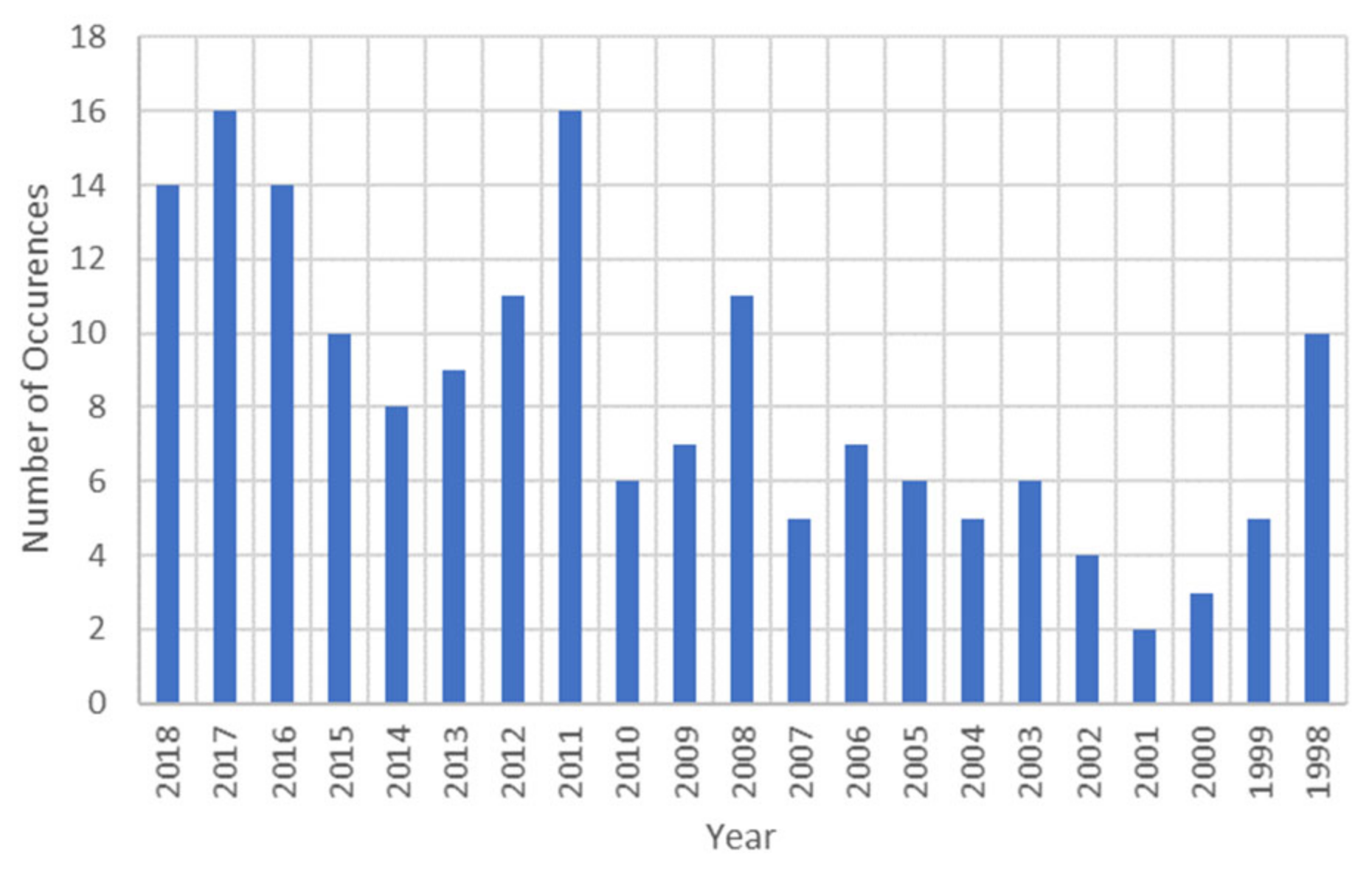
As the modern lifestyle becomes more electricity reliant, the conventional power distribution system faces challenges due to the rapid infiltration of distributed energy resources (DERs) and the increasing frequency of natural disasters [1]. The number of occurrences of major natural disasters per year that resulted in the loss of over $ 1 billion is shown in Figure 1. This figure clearly indicates the growing frequency of massive calamities [1]. Moreover, with a higher degree of electricity dependency, electric outages not only cause financial damage but also result in the loss of lives. Hurricane Irma provided a strong example where 29 out of 75 (39%) total deaths were due to power-related causes [2] (see

Table 1. Human casualties in Hurricane Irma [2].

Total Power Related	29
Outages	14
CO poisoning	11
Electrocution	2
Other	2
Drowning	7
Other	39
Total Deaths	75

). Hence, the modernization of the power grid in order to address such critical issues requires urgent attention. The deployment of microgrids (MGs) to improve grid reliability has been conceptualized as one of the solutions [3].

Recent developments in microgrid technology have added different functions, such as improving reliability, supply-demand balance, and economic dispatch, to create what has been called advanced microgrid (AMG) systems by Cheng et al. in [3]. The systems, such as AMG, introduce a three-tier hierarchical control structure where primary controls include protection, converter output control, voltage and frequency regulation, power sharing, and operation in the millisecond range [4,5,6]. The secondary controls consist of the energy management systems (EMSs), which can be viewed as multi-objective optimization tools that take several inputs, such as load profiles, generation forecasts, and market information, and use them for specified objectives, such as cost mitigation, demand response management, and power quality maintenance [3]. The operating time for secondary controls can range from seconds to hours [3]. The proposed machine learning (ML)-based EMS replaces the traditional optimization methods with the objective of improving the power availability to critical loads during disasters and prolonged outages. Lastly, tertiary controls are the highest level controls, often enforced by the distribution system operator (DSO), and have the slowest time range of minutes to days [3]. Tertiary controls will be out of the scope of the current study, as the proposed solution is targeted for implementation in residential environments independent of the energy providers.

The AMGs have focused on several objectives, such as cost optimization, supply-demand management, integration of DER, power quality maintenance, and the improvement of the reliability and resilience of the entire grid. However, limited attention has been dedicated to the improvement of power delivery to critical loads during disasters and prolonged outages. The load curtailing concept presented in [3] requires either communication with the DSO during contingencies or additional predictive algorithms to estimate the time to recover (TTR). Furthermore, the model requires continuous updating, which is computationally expensive. A micro-grid formation concept is presented in [7], which shares the closest objective with this study. The authors have used mixed integer linear programming (MILP) to optimally create microgrids within the existing grid infrastructure using connection points that already exist. This study presents an effective solution but considers a different approach to the system-level solution rather than focusing on the functionality of the microgrid and respective EMS/optimization techniques. Furthermore, the initial capacity of each DER in this model can cause significant changes in the formation patterns.

The conventional EMSs utilize model predictive controls (MPCs) that rely on deterministic models [3]. The occurrence and consequences of natural disasters cannot be determined by deterministic models at the same time, a significant amount of DER infiltration at the end consumer level can cause discrepancies. Therefore, probabilistic models provide better solutions. Machine learning algorithms (MLAs) utilize the sample of trajectories gathered from interaction with a real system or simulation rather than depending on a deterministic model [8]. In [8], the authors prove that reinforcement learning (RL) can offer comparable performance with that of MPCs even when good deterministic models are available.

More recent interest in using machine intelligence for optimization and load scheduling has been presented in [9,10,11,12]. In [9], authors present a dueling deep Q-learning targeted towards emergency load shedding. The difference in the priority (reward function) leads to a more complicated algorithm and is limited to simulations; this article neglects the details of implementation. In [10], authors utilize Q learning to optimize the scheduling of electric vehicle charging. In [11,12], the authors propose different variations in Q-learning to achieve objectives, such as improving the profit margin and microgrid interconnection. While these studies establish that Q-learning can be an effective algorithm to be considered for various objectives within power distribution, the proposed study focuses on the objective of critical reliability improvement and provides an integrated real-time study with experimentation from both power and machine learning perspectives.

A solution for local microgrids with DER integration capabilities and machine intelligence has been suggested in [13]. This article is the continuation of the work presented in [13]. The objective of this study is to prove the feasibility of utilizing the Q-learning algorithm as the core of EMS targeted toward the improvement of critical reliability. The study includes the theoretical analysis, integrated simulation model, reliability analysis, and support of experimental results. In [13], the support vector machine (SVM) was used for EMS, whereas this study considers Q-learning due to its inherent advantages, including its unsupervised nature, continuous learning, and adaptability. Furthermore, [13] does not include any experimental verification, which is provided in this manuscript.

This paper is structured as follows: Section 2 describes the power electronics (PE) model of MPEI with its state space equations and discusses changes in the model with varying converter functionality. Section 3 describes the Q-learning-based EMS with Q-value generation, reward calculation, and flow chart for implementation. Section 4 describes the effect of EMS output on the functionality and system-level model of the MPEI. Section 5 and Section 6 provide simulation results and experimentations, respectively. Section 7 discusses the significance of the proposed method with experimental case studies. Section 8 includes the conclusion.

2. Power Electronics Model

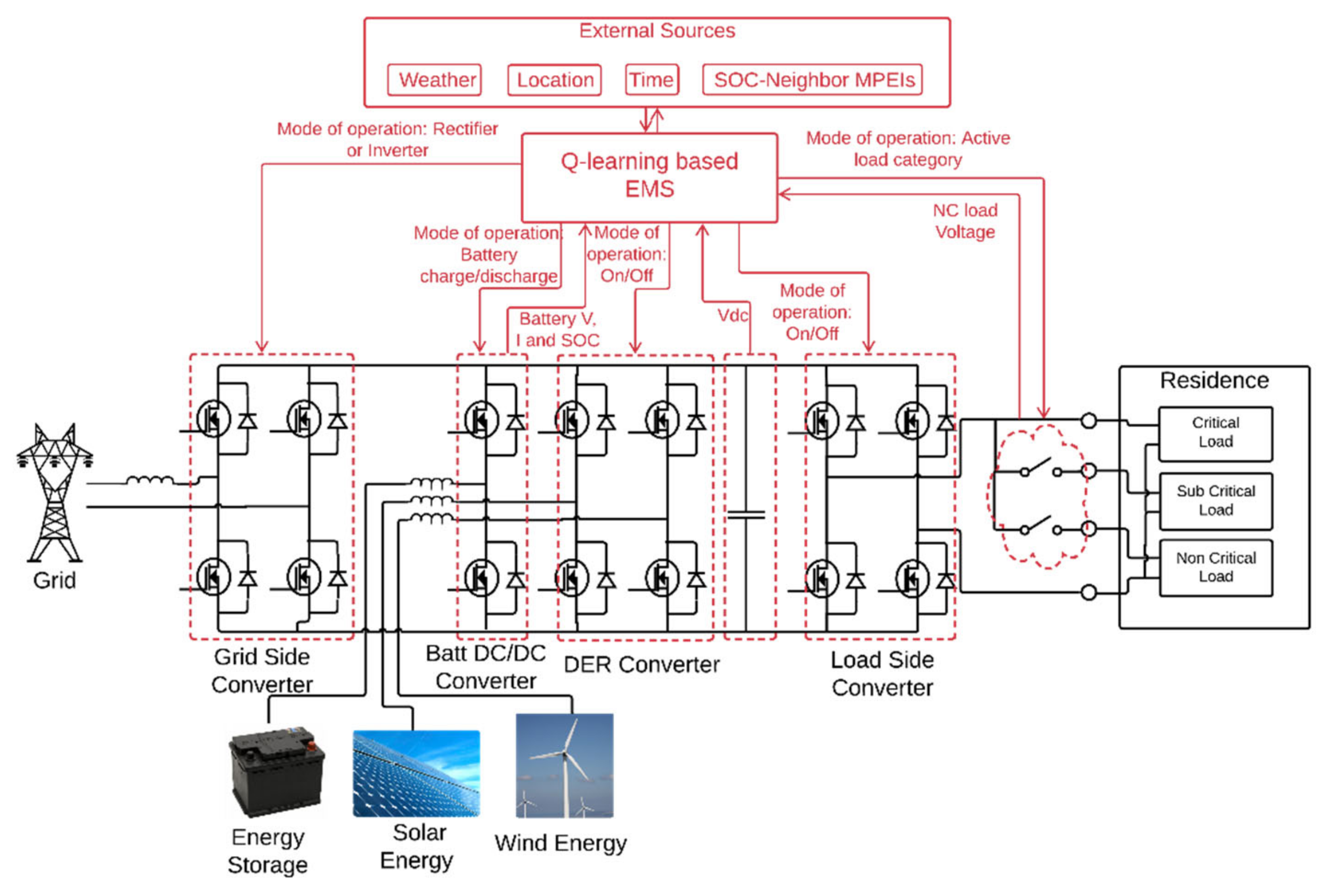
The foundation of the presented power electronics interface is based on the multi-port power electronics interface (MPEI) described in [14,15]. The version of MPEI that was considered and developed for this study is based on a single-phase system that includes four individual converters with load categorization capabilities, as described in [13]. Furthermore, the MPEI has the capability of incorporating the MLA outputs. The details and schematic are presented in Figure 2.

The four different converters that have been considered are the grid side converter (GSC), battery interface (BI), DER converter (DERC), and load side converter (LSC). This section provides the details for the derivation of the state space equation for GSC and lists the state space models for the rest of the converters generated using a similar procedure. The subscripts x and conv used in naming convention ${\psi }_{xy}, I_{Lconv}$ are listed in

Table 2. Subscript description table.

Converter	Subscript (x)	Mode	Value (conv)
GSC	g	Rectifier	1
		Inverter	2
BI	batt	Discharge	3
		charge	4
DERC	der	Boost	5
LSC	load	Inverter	6

.

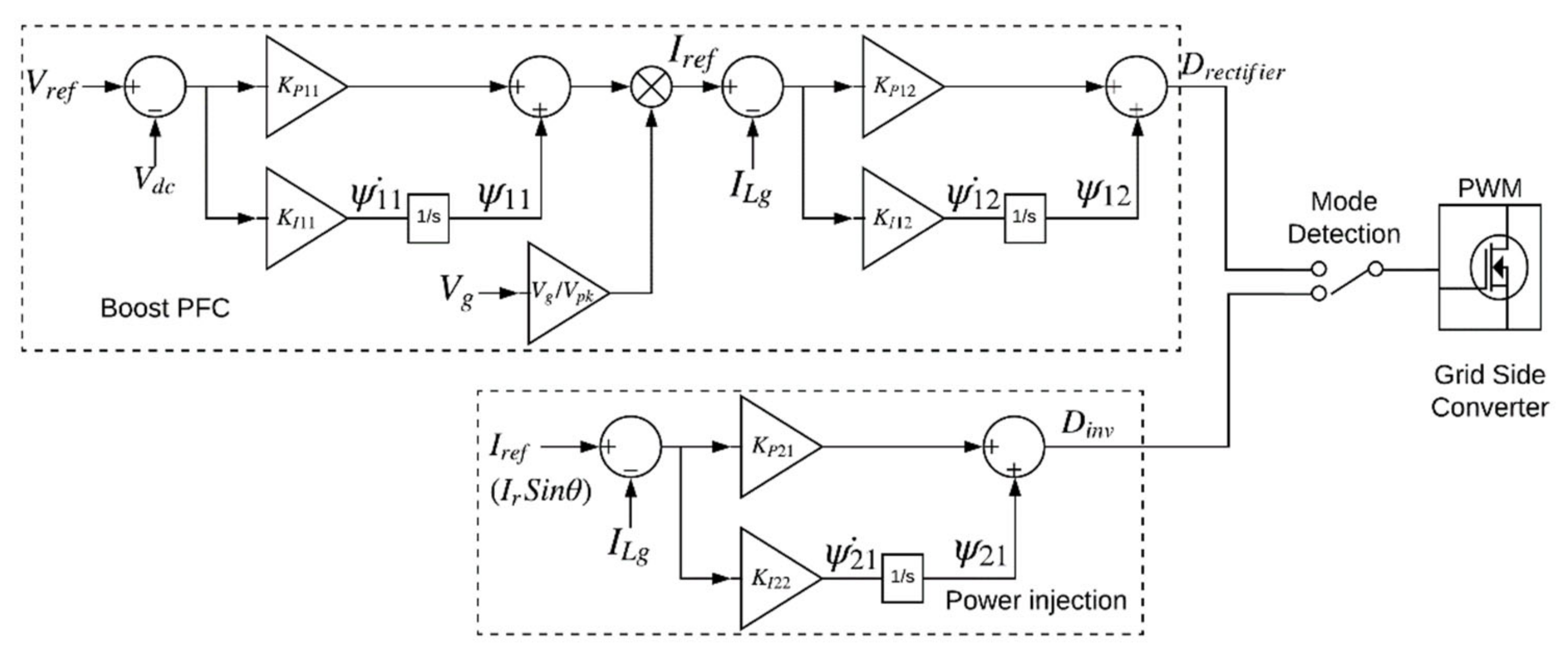
The GSC is a bidirectional converter that behaves as a rectifier with power factor correction (PFC) when the power flows from the grid to the DC bus and as an inverter when the power flows from the DC bus to the grid. The equivalent circuit of GSC while operating in rectifier and inverter modes has been included in [13]. The control schemes implemented for both modes are shown in Figure 3. The duty cycle-based weighted average state space equations can be generated. The parameters from the control schemes can be substituted into the average equations, and linearization can be performed to generate the complete state space models presented in Equations (1) and (2) for the rectifier and inverter modes, respectively [13].

The battery interface is also a bidirectional converter which behaves as a boost converter when the battery provides power to the DC bus and as a buck converter in the reverse direction. The procedure described for GSC can be used to generate the state space equations for BI as presented by Equations (4) and (5) for the discharge and charge modes, respectively. The details of BI have been documented in [13].

Similarly, the DERC is a unidirectional converter that resembles the boost mode of the BI and LSC is a unidirectional voltage mode inverter [13]. The state space equations for DERC, and the LSC are included as Equations (3) and (4).

$$\left[\begin{array}{c}\dot{\Delta {\psi }_{11}}\\ \dot{\Delta {\psi }_{12}}\\ \dot{\begin{array}{c}\Delta I_{Lg}\\ \dot{\Delta V_{dc}}\end{array}}\end{array}\right]=\left[\begin{array}{cccc}0& 0& 0& -K_{I11}\\ K_{I12}& 0& -K_{I12}& -K_{p11}{K}_{I12}\\ -\left(2V_{dc}{K}_{p12}\right)/L_g& -2V_{dc}/L_g& \left(2V_{dc}{K}_{p12}\right)/L_g& \left(1-2D-2V_{dc}{K}_{p11}{K}_{p12}\right)/L_g\\ 2I_{Lg}{K}_{p12}/C& 2I_{Lg}/C& \left(2D-2I_{Lg}{K}_{p12}-1\right)/C& -\left(2K_{p11}{K}_{p12}{I}_{Lg}+\left(1/R\right)\right)/C\end{array}\right] \left[\begin{array}{c}\Delta {\psi }_{11}\\ \Delta {\psi }_{12}\\ \Delta I_{Lg}\\ \Delta V_{dc}\end{array}\right]+ \left[\begin{array}{c}0\\ 0\\ 1/L_g\\ 0\end{array}\right]\Delta V_g$$

(1)

$$\left[\begin{array}{c}\dot{\Delta {\psi }_{21}}\\ \dot{\Delta I_{Lg}}\\ \dot{\Delta V_g}\end{array}\right]=\left[\begin{array}{ccc}0& -K_{I21}& 0\\ 2V_{dc}/L_g& -\left(2V_{dc}{K}_{p21}\right)/L_g& -1/L_g\\ 0& 1/C_g& -1/\left(Z_g{C}_g\right)\end{array}\right]\left[\begin{array}{c}\Delta {\psi }_{21}\\ \Delta I_{Lg}\\ \Delta V_g\end{array}\right]+\left[\begin{array}{c}0\\ \left(2D-1\right)/L_g\\ 0\end{array}\right]\Delta V_{dc}$$

(2)

$$\left[\begin{array}{c}\dot{\Delta {\psi }_{31}}\\ \dot{\Delta {\psi }_{32}}\\ \dot{\begin{array}{c}\Delta I_{Lbatt}\\ \dot{\Delta V_{dc}}\end{array}}\end{array}\right]=\left[\begin{array}{cccc}0& 0& 0& -K_{I31}\\ K_{I32}& 0& -K_{I32}& -K_{p31}{K}_{I32}\\ \left(V_{dc}{K}_{p32}\right)/L_{batt}& V_{dc}/L_{batt}& -\left(V_{dc}{K}_{p32}\right)/L_{batt}& \left(D-1-V_{dc}{K}_{p31}{K}_{p32}\right)/L_{batt}\\ -\left(I_{Lbatt}{K}_{p32}\right)/C& -I_{Lbatt}/C& \left(I_{Lbatt}{K}_{p32}+1-D\right)/C& \left(K_{p31}{K}_{p32}{I}_{Lbatt}+\left(1/R\right)\right)/C\end{array}\right]\left[\begin{array}{c}\Delta {\psi }_{31}\\ \Delta {\psi }_{32}\\ \Delta I_{Lbatt}\\ \Delta V_{dc}\end{array}\right]+ \left[\begin{array}{c}0\\ 0\\ 1/L_{batt}\\ 0\end{array}\right]\Delta V_{batt}$$

(3)

$$\left[\begin{array}{c}\dot{\Delta {\psi }_{41}}\\ \dot{\Delta I_{Lbatt}}\\ \dot{\Delta V_{batt}}\end{array}\right]= \left[\begin{array}{ccc}0& -K_{I41}& 0\\ V_{dc}/L_{batt}& -V_{dc}{K}_{p41}/L_{batt}& -1/L_{batt}\\ 0& 1/C_{batt}& -1/\left(R_{batt}{C}_{batt}\right)\end{array}\right]\left[\begin{array}{c}\Delta {\psi }_{41}\\ \Delta I_{Lbatt}\\ \Delta V_{batt}\end{array}\right]+\left[\begin{array}{c}0\\ D/L_{batt}\\ 0\end{array}\right]\Delta V_{batt}$$

(4)

$$\left[\begin{array}{c}\dot{\Delta {\psi }_{51}}\\ \dot{\Delta {\psi }_{52}}\\ \dot{\begin{array}{c}\Delta I_{Lder}\\ \dot{\Delta V_{dc}}\end{array}}\end{array}\right]=\left[\begin{array}{cccc}0& 0& 0& -K_{I51}\\ K_{I52}& 0& -K_{I52}& -K_{p51}{K}_{I52}\\ \left(V_{dc}{K}_{p52}\right)/L_{der}& V_{dc}/L_{der}& -\left(V_{dc}{K}_{p52}\right)/L_{der}& \left(D-1-V_{dc}{K}_{p51}{K}_{p52}\right)/L_{der}\\ -\left(I_{Lder}{K}_{p52}\right)/C& -I_{Lder}/C& \left(I_{Lder}{K}_{p52}+1-D\right)/C& \left(K_{p51}{K}_{p52}{I}_{Lder}+\left(1/R\right)\right)/C\end{array}\right]\left[\begin{array}{c}\Delta {\psi }_{51}\\ \Delta {\psi }_{52}\\ \Delta I_{Lder}\\ \Delta V_{dc}\end{array}\right]+\left[\begin{array}{c}0\\ 0\\ 1/L_{der}\\ 0\end{array}\right]\Delta V_{der}$$

(5)

$$\left[\begin{array}{c}\dot{\Delta {\psi }_{61}}\\ \dot{\Delta I_{Lload}}\\ \dot{\Delta V_{load}}\end{array}\right]= \left[\begin{array}{ccc}0& 0& -K_{I61}\\ 2V_{dc}/L_{load}& 0& -\left(1+2V_{dc}{K}_{p61}\right)/L_{load}\\ 0& 1/C_{load}& -1/\left(R_{load}{C}_{load}\right)\end{array}\right]\left[\begin{array}{c}\Delta {\psi }_{61}\\ \Delta I_{Lload}\\ \Delta V_{load}\end{array}\right]+\left[\begin{array}{c}0\\ \left(2D-1\right)/L_{load}\\ 0\end{array}\right]\Delta V_{dc}$$

(6)

The controller gains for each of the converters are chosen independently, and the stability of the converters is ensured individually by locating the poles of the resultant transfer function in the left-hand side plane. The controller gains and the respective poles for the converters are listed in

Table 3. Controller gain values and corresponding system poles.

		Kpv	Kiv	Kpi	kii	Pole 1	Pole 2	Pole 3	Pole 4
GSC	Rectifier	0.3	4.3	0.9	1000	−2.62 × 105	−1116.1	−24	−22.32
	Inverter	-	-	0.4	250	−1.19 × 105	−636.4	−332.4	-
BI	Discharge	0.3	3	5	100	−3.84 × 106	−36.8	−11.8	−11.2
	Charge	-	-	0.7	100	−4.40 × 105	−2.99 × 105	−142.9	-
DER	-	0.3	3	5	100	−3.84 × 106	−36.8	−11.8	−11.2
LSC	-	0.05	3	-	-	−13.5 + 5742.6i	−13.5 − 5742.6i	−62	-

. The converters are then integrated using a shared DC bus to create an MPEI. For this application, the behavior of the MPEI is a combined performance of the four converters discussed above. Hence, the characteristic of the MPEI varies with the operational mode of each of the converters, and the state space equation of the MPEI depends on the converter modes at the instant of consideration. There are 36 possible combinations of different modes for the four converters, as depicted in

Table 4. Modes of operation.

	State 1	State 2	State 3
GSC	Rectifier	Inverter	Off
BI	Discharge	Charge	Off
DERC	Boost	Off	-
LSC	Inverter	Off	-

. Each combination results in a different characteristic equation for the MPEI.

Considering the operational state of MPEI, where the modes of operation for the converters are as highlighted in

Table 5. k values, corresponding functions, and state space representation $\dot{Q_{xn}}$.

kx	1	2	3
GSC	Rectifier ($\dot{Q_{G1}}$)	Inverter ($\dot{Q_{G2}}$)	Off ($\dot{Q_{G3}}$)
Batt conv.	Discharge ($\dot{Q_{B1}}$)	Charge ($\dot{Q_{B2}}$)	Off ($\dot{Q_{B3}}$)
DER conv.	Off ($\dot{Q_{D1}}$)	Boost ($\dot{Q_{D2}}$)	-
Load inv.	Off ($\dot{Q_{l1}}$)	Inverter ($\dot{Q_{l2}}$)	-

, the state space model of the MPEI can be represented by Equations (7)–(11). The component matrices of the state space Equation (7) are included as Equations (8)–(11). The pole-zero diagram and the root locus for this state of MPEI are shown in Figure 4a and Figure 4b, respectively. Notably, there are a pair of complex conjugate poles stemming from LSC. These poles can potentially initiate an underdamped oscillatory response. It is important to select the controller gains so that the closed loop poles of the system can be real and stable. As the operational state changes, the mode of operation for each converter changes leading to a different set of state space equations. Once the characteristic equation of the MPEI is determined, the stability analysis can be performed on the complete power electronics system. More details are documented in [15,16].

$$\begin{gathered} \dot{x}=Ax+Bu \\ y=Cx+D \end{gathered}$$

(7)

$$x_{Mode1}=\left[\begin{array}{ccccccccccccc}\Delta {\psi }_{11}& \Delta {\psi }_{12}& \Delta I_{Lg}& \Delta {\psi }_{41}& \Delta I_{Lbatt}& \Delta V_{batt}& \Delta {\psi }_{51}& \Delta {\psi }_{52}& \Delta I_{Lder}& \Delta {\psi }_{61}& \Delta I_{Lload}& \Delta V_{load}& \Delta V_{dc}\end{array}\right]\prime$$

(8)

$$u_{Mode1}=\left[\Delta V_g\hspace{1em}\Delta V_{der}\right]\prime$$

(9)

$$A_{Mode1}=\left(\begin{array}{ccccccccccccc}0& 0& 0& 0& 0& 0& 0& 0& 0& 0& 0& 0& -K_{I11}\\ K_{I12}& 0& -K_{I12}& 0& 0& 0& 0& 0& 0& 0& 0& 0& -K_{p11}{K}_{I12}\\ \frac{2V_{dc}{K}_{p12}}{L_g}& \frac{2V_{dc}}{L_g}& \frac{-2V_{dc}{K}_{p12}}{L_g}& 0& 0& 0& 0& 0& 0& 0& 0& 0& \frac{2D_g-1-2V_{dc}{K}_{p11}{K}_{p12}}{L_g}\\ 0& 0& 0& 0& -K_{I41}& 0& 0& 0& 0& 0& 0& 0& 0\\ 0& 0& 0& \frac{V_{dc}}{L_{batt}}& \frac{-V_{dc}{K}_{p41}}{L_{batt}}& \frac{-1}{L_{batt}}& 0& 0& 0& 0& 0& 0& \frac{D_{batt}}{L_{batt}}\\ 0& 0& 0& 0& \frac{1}{C_{batt}}& \frac{-1}{R_{batt}{C}_{batt}}& 0& 0& 0& 0& 0& 0& 0\\ 0& 0& 0& 0& 0& 0& 0& 0& 0& 0& 0& 0& -K_{I51}\\ 0& 0& 0& 0& 0& 0& K_{I52}& 0& -K_{I52}& 0& 0& 0& -K_{p51}{K}_{I52}\\ 0& 0& 0& 0& 0& 0& \frac{V_{dc}{K}_{p52}}{L_{der}}& \frac{V_{dc}}{L_{der}}& \frac{-V_{dc}{K}_{p52}}{L_{der}}& 0& 0& 0& \frac{D_{der}-1-V_{dc}{K}_{p51}{K}_{p52}}{L_{der}}\\ 0& 0& 0& 0& 0& 0& 0& 0& 0& 0& 0& -K_{I61}& 0\\ 0& 0& 0& 0& 0& 0& 0& 0& 0& \frac{2V_{dc}}{L_l}& 0& \frac{-(1+2V_{dc}{K}_{p61)}}{L_l}& \frac{2D_l-1}{L_l}\\ 0& 0& 0& 0& 0& 0& 0& 0& 0& 0& \frac{1}{C_l}& \frac{1}{R_l{C}_l}& 0\\ \frac{-2K_{p12}{I}_{Lg}}{C}& \frac{-2I_{Lg}}{C}& \frac{1-2D_g+2K_{p12}{I}_{Lg}}{C}& 0& 0& 0& \frac{-K_{p52}{I}_{Lder}}{C}& \frac{-2I_{Lder}}{C}& \frac{1-D_{der}+K_{p52}{I}_{Lder}}{C}& 0& 0& 0& \frac{Q}{C}\end{array}\right)$$

(10)

$$\begin{gathered} \begin{array}{cc}{B}_{Mode1}=\left(\begin{array}{cc}0& 0\\ 0& 0\\ \frac{1}{L_g}& 0\\ 0& 0\\ 0& 0\\ 0& 0\\ 0& 0\\ 0& 0\\ 0& \frac{1}{L_{der}}\\ 0& 0\\ 0& 0\\ 0& 0\\ 0& 0\end{array}\right)& C_{Mode1}=\left[ 0 0 0 0 1 0 0 0 0 0 1 1\right] \\ {D}_{Mode1}=\left[ 0 0 \right]\end{array} \end{gathered}$$

(11)

3. Energy Management System

As mentioned in the introduction, the Q-learning-based EMS (QEMS) implemented in this study is an MLA-based EMS. The MLA explored for this study is the Q-learning algorithm. Q-learning is a model-free reinforcement learning method that follows the Markov decision-making process. The Q-learning algorithm views MPEI as an agent that implements the controlled Markov process with the goal of selecting an optimal action for every possible state [17].

The Q-learning operates by using three simple steps: reward calculation, Q value update, and locating the maximum rewards. The reward calculation is the user-set criteria that assign either a positive reward for desirable results or a negative penalty for undesirable results. A multitude of parameters can be chosen for reward calculation depending on the application. This is discussed in more detail in the following paragraphs. The Q value is the value stored in the Q table and is generated using Equation (12) [17], where $x_n$ is the current state, $a_n$ is the action performed, $y_n$ is the subsequent state, $r_n$ is the immediate reward, $Q_n$ is the new Q value, $Q_{n-1}$ is the previous Q value, and ${\alpha }_n$ is the learning factor, most often chosen to be very close to 1. Lastly, the maximum Q value for a particular state is chosen using the argmax function, as shown in Equation (13). This article will not include extensive discussions of Q-learning algorithms as more details are provided by Watkins in [17].

$$Q_n\left(x,a\right)=\left\{\begin{array}{l}(1-a_n)Q_n\left(x,a\right)+a_n{r}_{n}ifx=x_{n}anda=a_n\\ Q_{n-1}\left(x,a\right)\hspace{1em}\hspace{1em}\hspace{1em}\hspace{1em}\hspace{1em}\hspace{1em}\hspace{1em}\hspace{1em}\hspace{1em}otherwise,\end{array}\right.$$

(12)

$$\begin{gathered} a=\mathrm{argmax}\left(Q_n\right) \\ where, argmax f\left(x\right)≔\{x |\forall y:f\left(y\right)\le f\left(x\right) \end{gathered}$$

(13)

The Q table considered for this application consists of all the possible states of the input features as the rows and all possible actions as the columns. The input features that have been considered are weather, time, grid voltage, the state of charge (SoC) of the battery, and the SoC of neighboring battery storage systems. For simplification, the binary states of “good” or “bad” have been chosen for each of these features. Hence, the total number of possible states with given features is 2⁵ (32). The actions are the modes of the MPEI or are the combined result of the four different converters operating in different modes. As discussed in Section 2, the total number of possible actions is 36. Reducing the possible modes of the BI to discharge and charge only and eliminating the turn-off function reduces the number of actions to 24. Therefore, the Q-table for this application is a 32 × 24 matrix.

Reward calculation is an important step that assigns the parameters of interest, and priorities and, most importantly, allows for dictating the behavior of Q-learning algorithms to fit the application at hand. The objective of this study is to explore the feasibility of Q-learning algorithms when used as EMSs. EMSs can have complex multi-objective goals, but for proof-of-concept purposes, this study focuses on the single objective of reliability improvement. Since the LSC is directly connected to the DC bus, reliability translates to maintaining the DC bus to the desired value during all possible states. Hence, the main reward parameter is the DC bus voltage value. The bus voltage reward value is generated using a threshold detection method, as shown in Figure 5a. The Q-learning algorithm penalizes the action with −40 points if the DC bus voltage drops below 170 V. The second parameter of interest is the SoC of the battery. The SoC reward is generated using a continuous function—a bell-shaped curve with a maximum at 80% SoC and a lower limit of −28 at 50% and below, as shown in Figure 5b. The total reward is the cumulative value of both rewards.

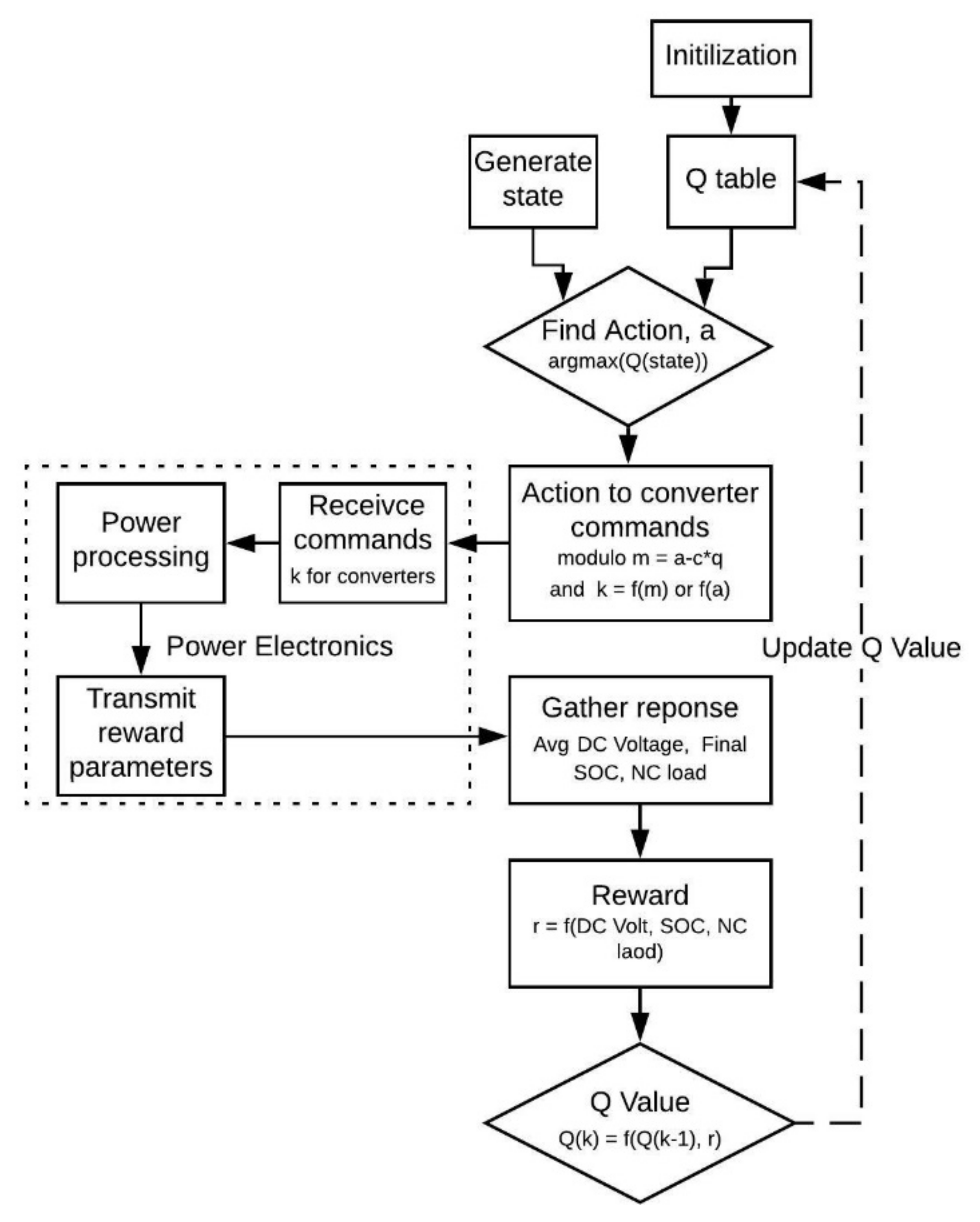
The flow diagram for the operation of the implemented Q-learning-based EMS is shown in Figure 6. The Q-learning algorithm first detects the input features to generate the state. Once the input state is detected, the corresponding row of the Q-table is scanned using Equation (13) to locate the column with the maximum reward. The resultant column number is named the action value, a, in this article. The a value then gets communicated to the MPEI, where it is translated to specific operational functions for each of the converters. Once the corresponding power conversion occurs, the response is recorded, and the reward parameters are communicated back to the EMS. The reward is then calculated, and the Q-value for the particular element of the Q-table is updated using Equation (12). The process is continually repeated. The Q-table is initialized with all zeroes, and if the maximum Q-value repeats in a row, argmax picks the column where it encounters the value for the first time.

4. Theoretical Integration

As discussed in Section 2, the MPEI can have different state space equations based on the mode of operation for the converters. The mode of the converters depends on the output of the Q-learning algorithm and the a value. The theoretical integration of MPEI and Q-learning depends on how the a value is translated to the commands for each of the converters and thereby allows for the determination of characteristic equations of the MPEI directly from the Q-learning output. This simplifies the process of performing the stability analysis by considering only the active converter modes.

The command for each of the converters is indicated with $k_x$ where x is the subscript corresponding to the converter (g represents GSC, b represents BI, and so on). For instance, k_g = 1,2,3 refer to GSC operating in the rectifier mode, inverter mode, and turned off, respectively. The $k_x$ values for each of the converters are described in Table 5. Furthermore, $\dot{Q_{xn}}$ represents the state space equation for each of the converters, as shown in Table 5 and Equation (14). The $\dot{Q_{G1}}$ represents the state space model of the GSC in rectifier mode, which can be obtained by expanding the corresponding equation included in Equation (14) to Equation (1). The state space equations for the rest of the converters in different modes can be obtained similarly.

The $k_x$ values for each of the converters can be obtained by using Heaviside step functions together with modular arithmetic. The Heaviside function is defined by Equation (15) where h(x) is 0 for x ≤ 0 and 1 for x > 0. The value of $k_g$ for GSC is determined directly using Equation (16), where k_g = 1 for a < 8, k_g = 2 for 8 ≤ a < 16, and k_g = 3 for a ≥ 16. This value of k_g determines the operation of GSC as shown in Table 4. For the remaining converters, modular arithmetic is used in addition to the Heaviside function, as shown in Equations (17) and (18), where m, c, and q are all positive integers, and q is the maximum possible value for each a. Each converter is assigned with a different value of c, the parameter m is then calculated using c, and m is finally used to calculate k_x. For instance, when a = 7, for GSC: k_g = 1, for BI: m = 3 (since c = 4), k_b = 2, for DERC: m = 7, k_d = 2, and for LSC: m = 1, k_l = 2. The output of the Q-learning algorithm can hence be translated into commands for each converter in MPEI.

Furthermore, each k_x value is also associated with converter equations $\dot{Q_{xn}},$ and the combination of individual equations, $\dot{Q_{Gk}}, \dot{Q_{Bl}}, \dot{Q_{Dm}}, \dot{Q_{Ln}}$ determines the total system equation for the MPEI. This can be represented as Equation (19), where the components of the leading matrices g₁, g₂, g₃, b₁, b₂, b₃, d₁, d₂, l₁, l₂ have values of 1 or 0 depending on the output of the Q-learning. The leading matrices are all initialized with 0 s. Once the k_x values are determined, the nth component of the leading matrices is replaced by 1 where n = k_x, as shown in Equation (18). For the scenario when a = 7, Equation (19) can be simplified to Equation (20), which can be further expanded using Equations (1)–(6), resulting in Equations (8)–(11). The stability and control analysis can then be performed for the MPEI for this particular mode without considering all the possible combinations. Similarly, if the scenario was to change to a = 20, the system equations for MPEI would change to a scenario where the GSC is off, BI is discharging, DERC and LSC are on, and the equations are presented in [16]. Hence, the system characteristics of the MPEI vary with the output (action value) of the Q-learning algorithm.

$$\begin{gathered} \dot{Q_{G1}}=\left[\begin{array}{c}\dot{\Delta {\psi }_{11}}\\ \dot{\Delta {\psi }_{12}}\\ \dot{\begin{array}{c}\Delta I_{Lg}\\ \dot{\Delta V_{dc}}\end{array}}\end{array}\right],\dot{Q_{G2}}=\left[\begin{array}{c}\dot{\Delta {\psi }_{21}}\\ \dot{\Delta I_{Lg}}\\ \dot{\Delta V_g}\end{array}\right],\dot{Q_{B1}}=\left[\begin{array}{c}\dot{\Delta {\psi }_{31}}\\ \dot{\Delta {\psi }_{32}}\\ \dot{\begin{array}{c}\Delta I_{Lbatt}\\ \dot{\Delta V_{dc}}\end{array}}\end{array}\right], \dot{Q_{B2}}=\left[\begin{array}{c}\dot{\Delta {\psi }_{41}}\\ \dot{\Delta I_{Lbatt}}\\ \dot{\Delta V_{batt}}\end{array}\right], \\ \dot{Q_{D2}}=\left[\begin{array}{c}\dot{\Delta {\psi }_{51}}\\ \dot{\Delta {\psi }_{52}}\\ \dot{\begin{array}{c}\Delta I_{Lder}\\ \dot{\Delta V_{dc}}\end{array}}\end{array}\right], \dot{Q_{l2}}=\left[\begin{array}{c}\dot{\Delta {\psi }_{61}}\\ \dot{\Delta I_{Lload}}\\ \dot{\Delta V_{load}}\end{array}\right], \\ \dot{Q_{G3}}=\dot{Q_{B3}}=\dot{Q_{D1}}=\dot{Q_{l1}}=0 \end{gathered}$$

(14)

$$h\left(x\right)=\begin{array}{l}0 for x<0\\ 0 for x=0\\ 1 for x>0\end{array}$$

(15)

$$k_g=h\left(a-7\right)+h\left(a-15\right)+1$$

(16)

$$\begin{gathered} m=a-c\ast q \\ where m,c,q \in {\mathbb{Z}}^{+} \& 0\le m\le \left(b-1\right) \end{gathered}$$

(17)

$$\begin{gathered} LSC: c=2, m=a-c\ast q, k_l=m+1, l_n=1 for n=k_l \\ BI: c=4, m=a-c\ast q, k_b=h\left(m-1\right)+1, b_n=1 for n=k_b \\ DER: c=8, m=a-c\ast q, k_d=h\left(m-3\right)+1, d_n=1 for n=k_d \end{gathered}$$

(18)

$$System eq.=\left[\begin{array}{ccc}{g}_1& g_2& g_3\end{array}\right]\left[\begin{array}{c}\dot{Q_{G1}}\\ \dot{Q_{G2}}\\ \dot{Q_{G3}}\end{array}\right]+\left[\begin{array}{ccc}{b}_1& b_2& b_3\end{array}\right]\left[\begin{array}{c}\dot{Q_{B1}}\\ \dot{Q_{B2}}\\ \dot{Q_{B3}}\end{array}\right]+\left[\begin{array}{cc}{d}_1& d_2\end{array}\right]\left[\begin{array}{c}\dot{Q_{D1}}\\ \dot{Q_{D2}}\end{array}\right]+\left[\begin{array}{cc}{l}_1& l_2\end{array}\right]\left[\begin{array}{c}\dot{Q_{L1}}\\ \dot{Q_{L2}}\end{array}\right]$$

(19)

$$System eq.=\left[\begin{array}{ccc}1& 0& 0\end{array}\right]\left[\begin{array}{c}\dot{Q_{G1}}\\ \dot{Q_{G2}}\\ \dot{Q_{G3}}\end{array}\right]+\left[\begin{array}{ccc}0& 1& 0\end{array}\right]\left[\begin{array}{c}\dot{Q_{B1}}\\ \dot{Q_{B2}}\\ \dot{Q_{B3}}\end{array}\right]+\left[\begin{array}{cc}0& 1\end{array}\right]\left[\begin{array}{c}\dot{Q_{D1}}\\ \dot{Q_{D2}}\end{array}\right]+\left[\begin{array}{cc}0& 1\end{array}\right]\left[\begin{array}{c}\dot{Q_{L1}}\\ \dot{Q_{L2}}\end{array}\right]$$

(20)

5. Simulation

The simulation of the system with the Q-learning algorithm and MPEI has been performed using Simulink. The MPEI model consists of four different converters, as described in Section 2. The complete MPEI model has been described in detail in [13]. The same Simulink model has been utilized in this study as well. However, in [13], the simulation is rooted in the Simulink platform, where the different blocks for power electronics, communication, and machine learning have been included in the model. The support vector machine (SVM) was implemented using the Matlab classification learner application. In this study, the Q-learning algorithm has been scripted as an m-file, which generates the input features, performs the Q-learning algorithm, initializes and runs the Simulink-based MPEI model, and calculates and updates the rewards.

The Q-table is initialized with all zeros. Before the successful implementation of the Q-learning algorithm, the Q-table must be filled with appropriate reward values. This process is called training. Training is most often conducted in a controlled lab environment prior to deployment. For training purposes, the input features are randomly generated, and, in other words, the input states of the iterations are randomly determined. The simulated system has 36 total states with 24 different actions; hence, each state has to occur at least 24 times before the completion of training. Thus, the least number of iterations required is 864 (24 × 36). A total of 2550 iterations have been performed to ensure that the Q-table is appropriately populated. A workstation with 16 cores was used, where 15 cores were operated in parallel to reduce the computation time.

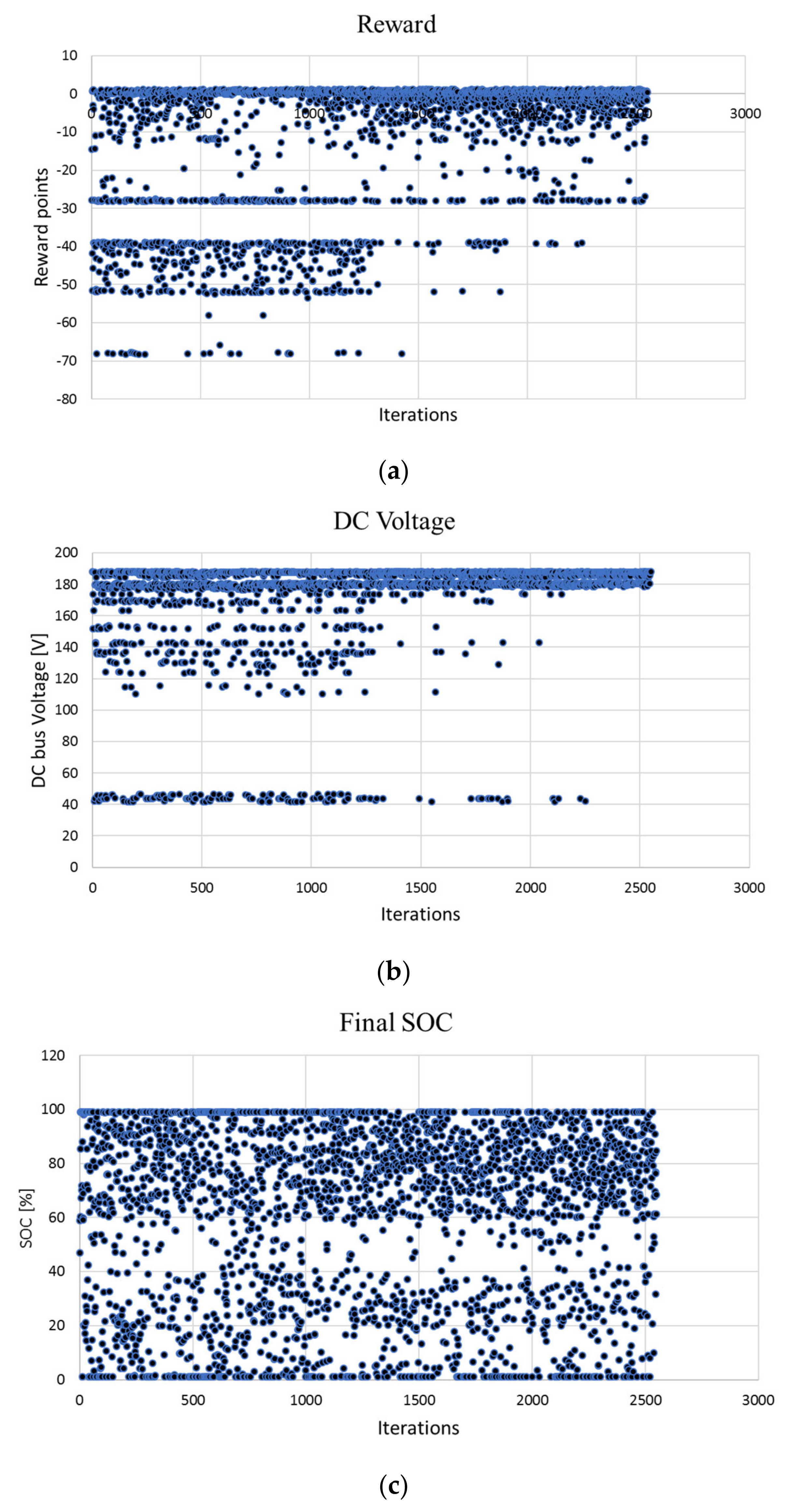
Since the MPEI model used in this study and [13] is identical, the stability and dynamics of the MPEI at different modes can be confirmed using the results presented in [13]. The more important outcomes of the Q-learning-based simulations are the results at the end of iterations that confirm the learning capability and performance of the Q-learning algorithm. Figure 7a–c shows the total rewards, minimum DC bus voltages, and the SoC of the battery at the end of each iteration. The reward values were calculated as discussed in Section 3 and are presented in Figure 5. The Q-table is initialized with all zeros, and the input features are randomly chosen. Therefore, with the increase in iterations, the reward values are expected to increase (less negative), the DC bus voltage is expected to be maintained at a nominal value, and the final SoC of the battery should be determined by Figure 5b. These trends can be observed in the results presented in Figure 7a–c.

The reward value is the sum of the DC bus voltage reward and the final SoC-based reward in Figure 5. Hence, the maximum possible penalty for this simulation is −68. If the system maintains the DC bus voltage, but the final SoC falls below 50%, then the reward is −28, and if the final SoC is 80% but the DC bus voltage is below 170 V, then the resultant penalty is −40. These values can be clearly as seen in Figure 7a. The stepwise nature of the DC bus reward and the lower limit of the SoC reward results in the steps for the total reward distribution. The continuous nature of the SoC reward (inverse parabola) for the final SoC greater than 50% contributes towards the values between the steps. More importantly, as seen from Figure 7a, highly negative penalties start disappearing as the number of iterations increases indicating that the Q-learning algorithm is learning and making corrective decisions while increasing the number of iterations.

Such trends can also be observed in the iterative distribution of the DC bus voltage. During the initial iterations, one can see that the frequency of the DC bus voltage dropped below the threshold of 170 V, which is very high. The bus voltage becomes more stable as the number of iterations increases, and it can be seen that after about 2000 iterations, the DC bus voltage drops only in six out of 550 iterations. Hence, the probability of obtaining a stable DC bus voltage using this system, considering all the possible scenarios, is about 0.989.

Lastly, Figure 7c presents the final SoC recorded at the end of each iteration. The power electronics simulation runs for 0.3 s, but the time has been scaled such that 0.3 s of charging or discharging affects the total SoC of the battery by 6%. The initial SoC of the battery was chosen to be any random value between 0% and 100%; this provided the software with enormous amounts of selection options resulting in the requirement of a large number of iterations (2550). This is also the reason why the learning cannot be deciphered easily from the final SoC distribution. However, tracking the final SoC for one particular state reveals the improvement. The final SoC reward distribution has a lower limit starting at 50% SoC, which implies that the penalty for maintaining the battery SoC at 50% is the same as depleting it further. Hence, at a 50% initial SoC, the Q-learning algorithm commands the NC load to stay on even though the battery SoC is low. In practical applications, the discharge is turned off when SoC drops below a certain level; such protection has been implemented during experimentation.

Hence, the simulation results verify the successful training of the Q-learning algorithm and confirm the effective implementation. Furthermore, since the LSC is connected to the DC bus and is immune to fluctuations in the grid or any other source, the lower penalties and stable bus voltage towards the end of training (>2000 iterations) verify that using this Q-learning-based EMS can ensure the stable critical load voltage. As shown in Figure 7b, the proposed Q-learning-based EMS allowed the load voltage to drop only 7 times in the last 550 iterations. Assuming that the model is fully trained with 2000 iterations and that the grid voltage value is bad (below 170 V_pk) for half of the total iterations, the suggested EMS ensures the stability of the load voltage with an overall probability of 0.987. The probability of obtaining a stable load voltage when the grid is unavailable is 0.974. Therefore, it can be concluded that the critical reliability of the system can be improved by using the proposed EMS compared to existing systems without an intelligent EMS. A thorough comparison with other AMG studies has not been included as a part of this article since the current objective of this study is to prove the feasibility of Q-learning-based EMS and to realize the initial improvement in terms of critical reliability; comparisons will be performed as a part of future work.

The hereby developed algorithm will be used with the MPEI test bed for experimental verification in the following section.

6. Experimental Verification

The experimental setup includes an MPEI unit developed as discussed in Section 2, the Q-learning-based EMS with corresponding features of generation, scaling, and reward calculation techniques (written in MATLAB), and wireless communication between the EMS and MPEI.

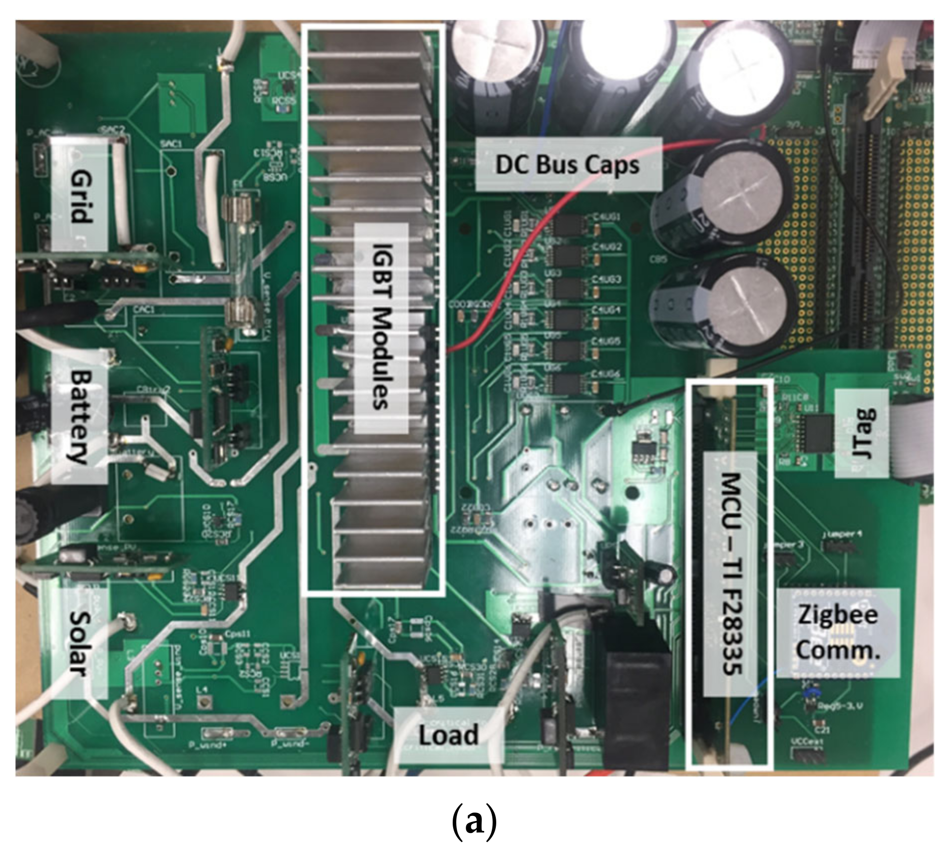
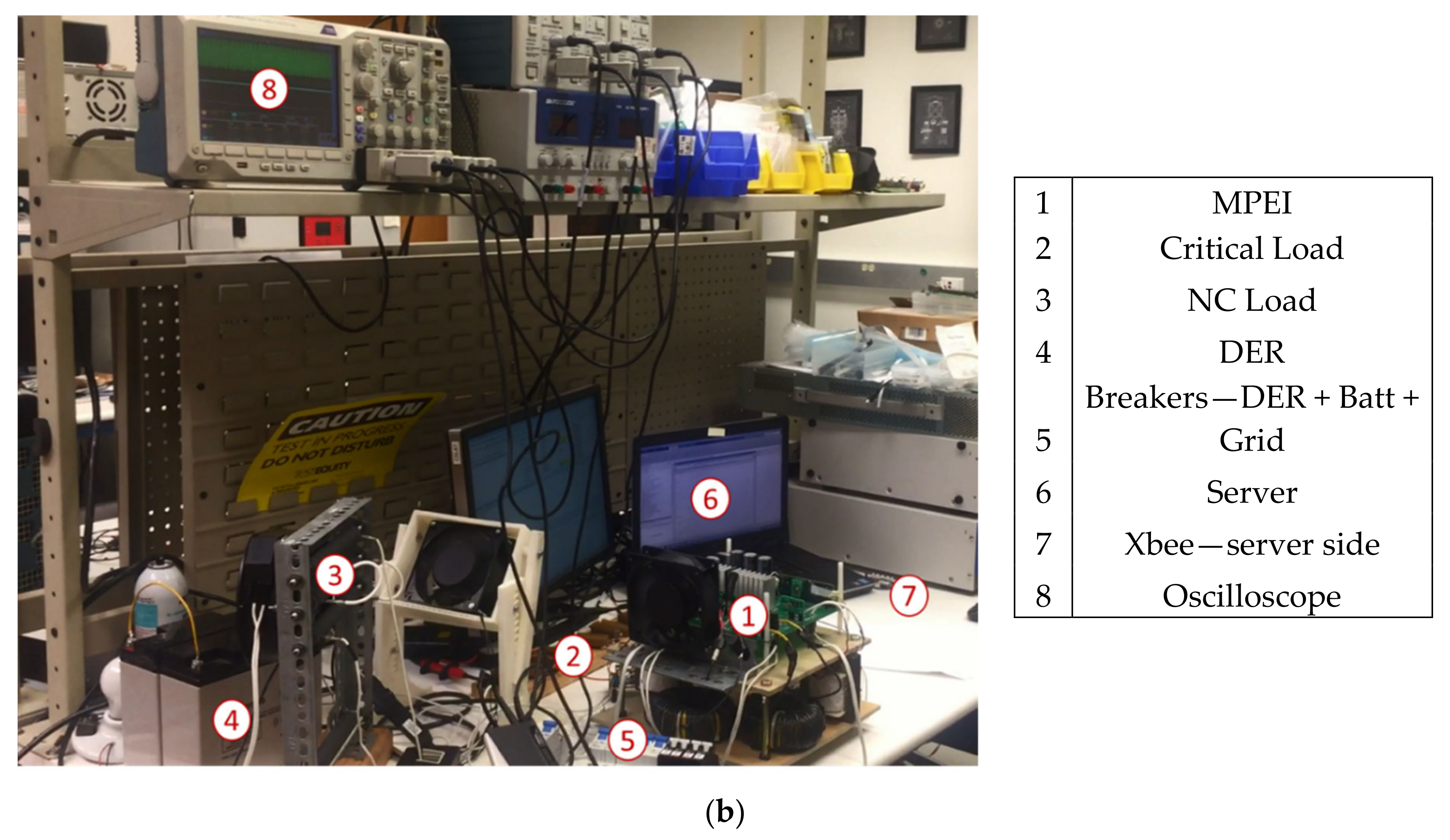
The 2 kW MPEI unit, designed as part of this study, utilizes two STGIPS30C60 IGBT modules with three bridge legs each and a TMS320F28335 micro controller unit (MCU). The details of the MPEI board are shown in Figure 8a. The MPEI consists of three different input sources labeled Grid, Battery, and Solar, and it has an output for the non-critical load. For this experiment, the critical load is directly connected to the DC bus. Therefore, the goal of ensuring stable power to the critical load can be translated as maintaining the DC bus voltage to the desired value. The communication between the MLA server and the MPEI is established wirelessly using Xbee S2C modules that are based on Zigbee protocols. The complete experimental setup is shown in Figure 8b. The DER was emulated using a smaller battery bank, shown by #4 in Figure 8b.

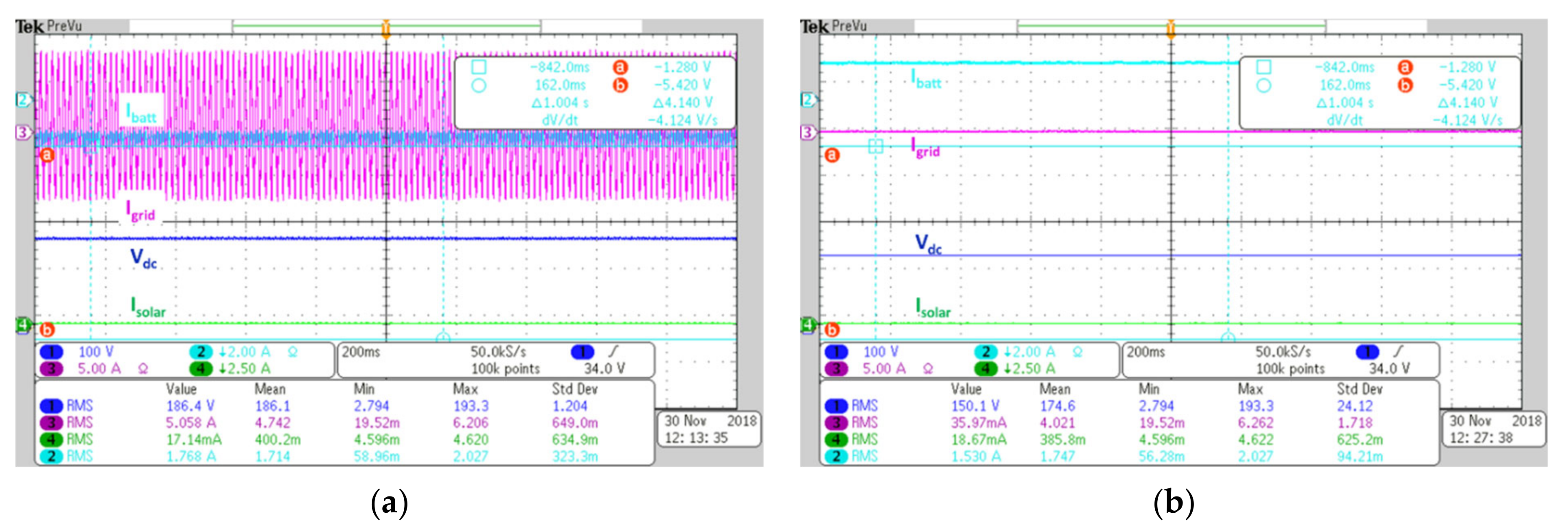
The MPEI was designed, developed, and tested without the EMS, the communication was established with the server, the Q-learning-based EMS was developed and implemented, and finally, the entire system was stabilized by manually varying the input states of the Q-learning algorithm. The results for one of such instances are shown in Figure 9a,b, where the grid, which is initially on, will turn off and turn back on. Figure 9b shows the transient response when the grid power comes back. The stable performance of the MPEI is apparent in Figure 9; a similar process was repeated for all the possible input states and output actions.

The experimentation was conducted for the verification of the simulation results. During simulation, the grid faults and the availability of DER (such as day and night for solar) could be created using the software. For the experimental results, these scenarios had to be created physically. The GSC and DERC were used to create such disruptions. This is equivalent to real operational scenarios, which dictate that GSC is on when the grid is available and DERC is on when enough solar energy is available. The functionality of GSC is reduced to the turned-off mode or rectification when the power injection to the grid has been disabled. This simplifies the Q-learning table to a 4 × 6 table. The possible states are now determined by the feasible combination of GSC and DERC and the actions of different combinations of BI and LSC. Hence, the Q-table looks similar to

Table 6. Q-table.

			Action
			BI: Charge	BI: Charge	BI: Discharge	BI: Discharge	BI: Off	BI: Off
			LSC: On	LSC: Off	LSC: On	LSC: Off	LSC: On	LSC: Off
			1	2	3	4	5	6
State	GSC: On	1	Sim: −1.373	−30.548	−11.925	−40.953	−11.482	−40.983
	DERC: Off		Exp: −0.794	−30.694	−12.004	−40.815	−9.5388	−41.338
	GSC: Off	2	Sim: −98.54	−127.79	−17.821	−141.49	−108.7	−137.76
	DERC: On		Exp: −128.05	−124.39	−38.981	−167.48	−70.91	−134.89
	GSC: Off	3	Sim: −98.503	−127.42	−33.844	−59.929	−108.76	−142.11
	DERC: Off		Exp: −130.97	−124.22	−51.357	−81.119	−141.19	−135.09
	GSC: On	4	Sim: −1.52	−30.649	−11.627	−40.833	−11.518	−40.709
	DERC: On		Exp: −1.45	−29.993	−12.824	−41.046	−11.01	−39.465

, where the function for each of the converters is outlined. Furthermore, from Section 5, one realizes the limitation of the SoC reward that was used. So, the SoC reward was modified to extend the lower limit to the final SoC of 25% rather than 50% and the lower limit penalty was changed to −150 points. The parabolic function was changed to assign the penalty of −45 for the final SoC of 50%, and the maximum reward close to 0 at 80%. However, the BI stops discharging if the SoC falls below 30% as protection; hence, 25% of the final SoC should never occur. The initial SoC was fixed to 65% in order to reduce the number of iterations required to train the algorithm. The DC bus voltage penalty value has been increased to −100 when the bus voltage falls below 150 V. Lastly, a reward category related to the non-critical load has been introduced in the non-critical load voltage is below the threshold (or the non-critical load is turned off), and the respective penalty of −30 is assigned. This has been added to prevent the unnecessary turn-off mode for the non-critical load.

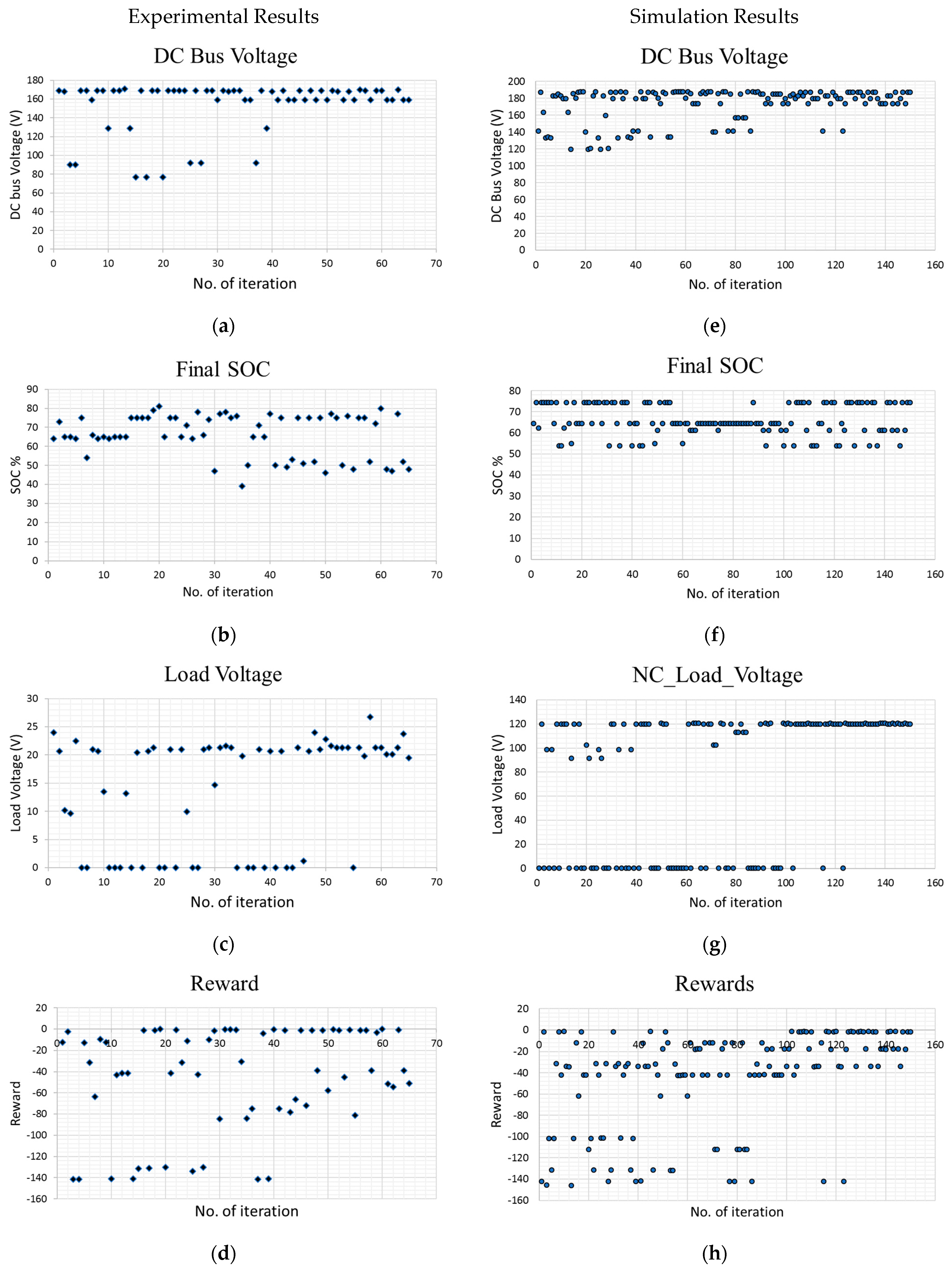
The experimentally obtained results are presented in Figure 10a–d and in Table 5. The first and most important observation is that the DC bus voltage never falls below the threshold after the 40th iteration. Since the critical load is connected directly to the DC bus, it does not experience instability after the 40th iteration. The two levels of the DC bus voltage exist because different references are assigned to GSC and BI (170 V and 160 V) in order to differentiate the action through the results. The final SoC has three distinct bands above and below the initial SoC of 65%, indicating that battery charges or discharges. As seen from Figure 10c, the non-critical load is kept on in most of the iterations towards the end. Finally, it is clear from Figure 10d that highly negative reward values disappear as the number of iterations increases indicating that the Q-learning algorithm is functioning and the training process is successful. The response of the system with a trained EMS for states 1 and 3 are shown in Figure 11a,b. In state 1, the grid power is available, so the GSC is on, and the solar is not available, so the DERC is off. As a result, the BI charges the battery indicated by a negative current, and LSC is on. This agrees with the response dictated by action 1 of the Q-table (gray cell). In state 3, both GSC and DERC are off, so as a result, BI discharges the battery (positive current) to maintain the DC voltage, and LSC is on as dictated by action 3 of the Q-table. The DC bus voltage does not drop below 150 V when the grid and DER power is cut off, indicating that EMS is performing effectively. Furthermore, once the Q-learning algorithms are trained, the DC bus voltage never drops except during the brief transient mode changes.

The simulation presented in Section 5 has been modified to replicate the experimental scenario. The results are presented in Figure 10e–h. There are two distinct differences between the simulation and experimental models. The first is that the simulation model consists of an exponentially decaying randomness factor (α) which is later deemed unnecessary while using strictly negative rewards; hence, it was removed from the experimental MLA. This results in a higher number of iterations required to train a model. The second is the amount of energy provided by the DER; a realistic model was created in the simulation where DER was capable of providing most of the required energy (83.33%) when the grid was off. However, since a secondary smaller battery bank was used during the experiment in the lab environment, the DER could only provide 24.91% of the required energy in such a scenario. This affects the final SoC of the battery, as discussed in the following paragraphs.

The most significant validation of the simulation results can be obtained by comparing the Q-table of the simulated and experimental models. The comparison is provided in Table 6. Table 6 consists of the possible states as rows and the actions of columns. For each state determined by the combination of the modes of GSC and DERC, the optimal action is determined by the lowest penalty in the corresponding row. This is highlighted in Table 6 with the gray background cells. As can be seen from Table 6, the actions determined for all four modes through the simulation and experiment are identical. This ensures that the proposed Q-learning algorithm performs consistently during the experiment and the simulation. The reward values in the Q-table are similar when the battery charges, while they show a significant mismatch when the battery discharges; this is due to the difference in the final SoC caused by a discrepancy in the capacity of DER and the size of the load. However, the difference in reward values has no effect on the performance of the algorithm as long as the column/action with a maximum reward for each of the states is the same. Furthermore, the penalties assigned to the second most favorable actions for each state are significantly higher than those assigned to the chosen actions, indicating strong selections in both cases.

The DC bus voltage obtained through the experiment and simulation is shown in Figure 10a and Figure 10e, respectively. The distributions of the DC bus voltage values match closely except for the number of iterations. The slight differences in the maximum and minimum voltage values are due to different references set in the simulation and experiment, which has no effect on the performance of the EMS. More significantly, the DC bus voltage is maintained above the threshold voltage with an increased number of iterations in both models, ensuring the successful implementation of the Q-learning-based EMS.

The final SoC values obtained from the experiment and simulation are shown in Figure 10b and Figure 10f, respectively. The final SoC values of the trained experimental model are represented by the samples for iterations greater than 40; they have two distinct values of around 50% and 75%, while there are three values for the simulation results, approximately at 52%, 62%, and 75%. This can be explained by considering the difference in energy provided by the DER when the GSC is off, as mentioned earlier. In the simulation, when GSC is off, the battery provides 16.67% of the total energy required, resulting in the SoC dropping of around 2.2% and forming the third distinct cluster at the SoC value of 62%. On the other hand, in the experiment, the battery still accounts for 75.09% of the total energy, resulting in around an 11% SoC drop which is very close to the SoC drop of 15% caused when the DER is not available. The closeness of the resultant final SoC values (54% and 50%), along with the communication noise, makes it appear as if they make one cluster with a larger margin of error, while they are the results of optimal actions at two different modes. The fluctuations of more than 4% can be noticed in Figure 10b.

The distribution for the simulated and experimental NC load voltages provided in Figure 10g and Figure 10c, respectively, present a close match. The NC load voltage reference values and LSC types are different in the simulation and experiment; however, this has no effect on the objective of the study. The communication disturbances are apparent in the experimental results as NC load voltages appear to fluctuate when LSC is on. In both cases, the EMS strives to keep LSC on more frequently as the number of iterations increases. This results in higher rewards for most of the modes when the initial battery SoC is 65%.

The total rewards for the simulation and experimental results can be compared from Figure 10d,h. The reward values are equal, and the distribution is similar. The reward points obtained from the experiment are more scattered than those from the simulation; this is the result of a difference in SoC, as discussed above, communication disturbances, and other anomalies. More importantly, the total reward decreases in magnitude as the number of iterations increases in both experiment and simulated results. This verifies the accuracy of the simulation model; hence, it validates the simulation-based analysis provided in Section 5.

7. Discussion

This section discusses the impact of the proposed technology on the reliability of the power distribution system. The distribution system reliability can be measured using metrics such as the system average interruption frequency index (SAIFI), system average interruption duration index (SAIDI), and expected energy not served (EENS). Since frequency-related metrics do not apply to the study at this stage, the system reliability and improvement have been measured in terms of the duration and energy available to the critical load, similar to SAIDI and EENS.

For reliability analysis, the setup described in Section 6 has been re-trained. The changes have been made for the proper implementation and simplification, as described in this paragraph. The EMS has been trained in island mode for a simplified and reduced training time. The initial SOC, which was considered to be fixed in Section 6, has been changed to four possible values of 35%, 55%, 75%, and 95%. Limiting the initial SOC to four possible values rather than a continuous value reduces the Q-table and allows faster training while providing enough data points for a valid justification. The combined SOC of the two batteries has been used as the system SOC as they share a common DC bus. The battery converters share a common functionality unless one of the battery SOCs falls below 31%; in this case, the battery converter turns off. The DER (solar) is used to charge the battery and provide a supporting current; the DER cannot meet the energy demand to maintain the DC bus voltage. The system starts load curtailing when SOC falls to 75% and disconnects all NC loads when SOC falls to 55%.

The Q-table has been attached as

Table A1. Q-table for reliability analysis in islanded mode.

MD/BC	1	2	3	4	5	6	7	8	9	10	11	12	Solar	SOC
1	−161.8	−162.08	−162.19	−162.06	−218.05	−225.21	−224.93	−231.62	−190.76	−199.99	−197.77	−206.38	On	35
2	−215.18	−215.25	−215.31	−215.34	−231.76	−231.77	−231.69	−231.91	−210.83	−213.14	−213.28	−213.1	Off	35
3	−116.5	−116.4	−116.62	−116.38	−89.81	−86.38	−84.73	−84.518	−124.76	−132.97	−131.67	−139.61	On	55
4	−144.75	−144.76	−144.69	−144.53	−201.9	−208.78	−208.46	−113.22	−143.35	−143.33	−143.47	−143.16	Off	55
5	−114.71	−114.4	−114.71	−114.59	−26.27	−28.19	−25.86	−27.41	−97.707	−104.54	−104.69	−111.62	On	75
6	−112.61	−112.58	−112.56	−112.69	−46.66	−44.88	−44.82	−43.83	−112.21	−112.2	−111.9	−112.49	Off	75
7	−151.42	−154.27	−151.18	−151.19	−0.54	−6.99	−6.89	−13.971	−109.31	−115.38	−116.32	−122.26	On	95
8	−119.47	−120.17	−119.48	−119.43	−5.47	−9.75	−9.07	−14.476	−120.75	−119.9	−120.62	−120.76	Off	95
Battery	Charge				Discharge				Off
NC ld1	On	On	Off	Off	On	On	Off	Off	On	On	Off	Off	53 W
NC ld 2	On	Off	On	Off	On	Off	On	Off	On	Off	On	Off	25 W

in Appendix A. Highlighted in red are the optimal rewards for each operational mode, which corresponds to the state of each variable represented by the grayed cells at the end rows and columns of the table. The results of implementing this Q-table are shown in Figure 12 below. Figure 12a presents the results for the experimental setup described in Section 6, where the total power consumption of the system is 206.3 W, the critical consumes 128 W, and the NC loads consume 53.3 W and 25 W each. The grey dotted line represents the grid without any microgrids, the dashed orange line represents the conventional microgrid with no load curtailing, and the solid blue line represents the microgrid with the proposed EMS. The power is cut off at t = t₀, and the power to the critical loads is immediately cut off for a traditional grid with no microgrids. The conventional microgrids with no load curtailing provide power to all the loads until the battery SOC depletes at t = t₃, at which point the power to the critical load is cut off as well. The proposed EMS keeps all the loads on until t = t_1, where the battery SOC falls below 75%. At t₁, the EMS starts load curtailing and disconnects NC load 1, the larger NC load. At t₂, the SOC drops to 55%, and all the NC loads are disconnected. The total SOC drops to 31% at t₄, and the critical load is disconnected. Compared to no microgrids, the proposed QEMS reduces the average interruption duration to the critical load from 18 h to 10 h. Compared to microgrids with no load curtailing, QEMS reduces the average interruption duration to the critical load from 12 h to 10 h; this indicates a SAIDI improvement of 16.66%.

However, it is important to consider that the critical to non-critical load ratio considered in the experiment above is exaggerated (128 W:78.3 W). Since the application is targeted at residential locations, the NC loads are expected to constitute the majority of the total load. Hence, the Q-table and experimental results in Figure 12a have been extended to represent a more realistic scenario where critical loads account for 20% of the total load. The total load is kept constant as in the previous case. The results are presented in Figure 12b. The average interruption duration for QEMS (t₅ − t₄) is now 3 h, which indicates a SAIDI improvement of 75%.

8. Conclusions

A Q-learning-based EMS targeted toward the improvement of critical reliability has been proposed. The feasibility of the implementation of the Q-learning algorithm as an EMS has been verified analytically, through simulation, and via experiment. The effect of the MLA output on the characteristic equations of the MPEI and subsequent simplification has been presented. The Q-learning algorithm has been developed and integrated with the simulation and experimental power electronics system. A multidisciplinary simulation model has been developed and integrated with the MLA code. The MPEI with three input power sources and two DC outputs has been developed with effective power routing capabilities and the ability to communicate with the server that runs MLA in real-time. Finally, the Q-learning-based EMS has been successfully integrated with the MPEI, and experimentation has been conducted with results that show a distinct reliability improvement. As can be seen from Figure 10a, the DC bus voltage never drops below the threshold after the training session is completed, ensuring that the critical load is powered during all possible scenarios. The consistency of the simulation and experimental results for the DC bus voltage, final SoC of battery, non-critical load voltage, and total rewards verifies the claimed improvement of the critical reliability and feasibility a Q-learning-based EMS brings. Figure 12a,b highlight the importance of the proposed technology, which includes load categorization, curtailing, and prioritization using intelligent EMS, especially in a future where more outages are predicted, and more human lives depend on the availability of electric power.