Abstract
Energy has become the most expensive and critical resource for all kinds of human activities. At the same time, all areas of our lives strongly depend on Information and Communication Technologies (ICT). It is not surprising that energy efficiency has become an issue in developing and running ICT systems. This paper presents a survey of the optimization models developed in order to reduce energy consumption by ICT systems. Two main approaches are presented, showing the trade-off between energy consumption and quality of service (QoS).
1. Introduction
1.1. Growth of Energy Consumption by Computing Systems: Reasons and Dynamics
The amount of energy consumed by computing and communication devices has increased rapidly. Although a lot of effort has been put into developing energy-efficient systems, the growing number of devices in use has resulted in an exponential rise in total Information and Communication Technologies (ICT) energy consumption in the 21st century [1]. The development of the IoT (Internet of Things) and the digital economy has increased the demand for ICT services [2,3]. Energy consumption by ICT is commonly divided into four main categories:
- consumer devices, including personal computers, mobile phones, TVs, and home entertainment systems;
- computer networks;
- data center computation and storage;
- production of ICT equipment.
The production of ICT equipment is beyond the scope of this paper, but we show the data in a broader context.
Figure 1 shows that compared to the beginning of the decade, the amount of energy consumed by consumer devices is expected to be similar to the amount of energy consumed by data centers, whereas consumer devices are expected to slightly decrease their energy consumption. The rapid development of cloud computing, as well as the Internet of Things, are possible explanations for this trend. Although some new data show that this prediction was overestimated [4], the available forecasts confirm that the general trend will not change in the next few years.
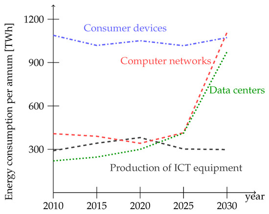
Figure 1.
Estimated annual ICT energy consumption. (Source: data from [4,6]).
It is expected (see Figure 2) that by 2030, almost half of the energy required by the ICT sector will be consumed by computer networks, mainly wireless networks. A lot of research has been devoted to this topic [5].
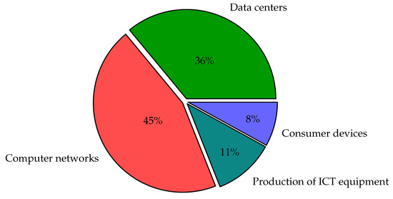
Figure 2.
Estimated proportion of energy consumption by ICT sectors in 2030 (Source: based on [7]).
1.2. Need for Energy Efficiency
The rapid growth of energy consumption is a reason for concern, especially given the energy crisis we are facing. At the same time, electrical power is used in all types of human activities including production, agriculture, construction, transportation, communication, healthcare, and leisure. ICT accounts for a significant share of energy consumption, including entertainment, television (TV), telephones, and media, and the estimated share of global ICT electricity consumption by 2030 has been estimated at 21% in a likely scenario and 51% in a worst-case scenario [6].
It is obvious that ICT should become sustainable in terms of energy [7,8,9]. There are at least three approaches that should be taken in parallel to achieve this goal. The first is the reduction of energy consumption. The second is the increased consumption of renewable energy to power ICT systems. The third is the use of waste heat from servers. Since energy has become such an expensive resource in recent years, the first approach seems to be the most economically efficient.
1.3. Ways to Reduce Energy Consumption by Computing Systems
Energy savings can be obtained in many ways depending on the considered system. The approaches presented in the literature usually address a single processor [10], a data center [11] (multiprocessor systems), and computer networks [5]. The energy used by ICT devices depends on their logic, architecture, and operation. Controlling system operations by assigning resources (processors, power) to jobs has proven to be very effective. Moreover, the methodology developed within the theory of scheduling is very useful in this context.
There are two general approaches to saving energy in computing systems. The first one is based on selecting a subset of cores, processors, or other elements of the infrastructure to be active in a given time period, allowing the remaining ones to switch to a sleep mode so that they do not consume energy. The other approach uses the fact that there is a relationship between power usage and job execution speed that can be used to balance energy consumption and computing efficiency.
In this paper, a survey of mathematical models useful for the design and operation of power-aware ICT systems is presented. We point out two issues that must be taken into account while modeling power-aware computing systems. The first is system performance. The methods used in order to reduce energy consumption must guarantee the required QoS, in particular, the computation time. The second issue is an effect of the Jevons paradox, namely that increasing the efficiency with which a resource is used leads to an increase in the total consumption of that resource due to decreasing costs.
This survey is restricted to CMOS technology since it is still the predominant technology in computing systems.
This paper is organized as follows. In Section 2, we show the approaches where the energy consumption of a computing system is decreased due to its logic, architecture, or by controlling the number of devices in use. Section 3 relates to a job model where the processing speed depends on the amount of resources (power) allotted to the job at a given time. From the point of view of modeling techniques, power-aware computing uses online and offline scheduling and discrete as well as continuous functions. Since usually realistic problems are NP-hard, solution algorithms are mainly heuristics. In Section 4, we discuss the features of modeling power as a discrete and continuous resource. The conclusions are summarized in Section 5.
2. Models That Switch Devices On and Off
As mentioned in Section 1.1, energy consumption by ICT systems is usually analyzed in four main areas: data centers, consumer devices, computer networks, and the production of ICT equipment. Each area faces specific challenges and opportunities for sustainable energy consumption. The energy efficiency of ICT systems became a research topic some years ago [12,13,14,15,16,17]; especially demanding is the optimization of energy consumption in high-performance computing systems [18].
2.1. Processor
Currently, a complementary metal-oxide semiconductor (CMOS) is the predominant technology used to construct integrated circuit (IC) chips including microprocessors, microcontrollers, memory chips, and other digital logic circuits [19]. Moreover, analog circuits, such as RF circuits, image sensors, data converters, and highly integrated transceivers for many types of communications, also use CMOS technology. In this section, we focus on the power performance trade-off between CMOS processors and costs. We start with a well-known model [10,20] consisting of three related equations. Power usage is defined by the first Equation (1).
The first term represents the dynamic power usage caused by the charging and discharging of the capacitive load on each gate’s output, which is proportional to the frequency of the system’s operation, f, the activity of the gates of the system, A, the total capacitance seen by the gate’s outputs, C, and the square of the supply voltage, V. The second term measures the power used as a result of the short-circuit current, , which flows between the supply voltage and ground at the moment when a CMOS logic gate’s output switches. The third term captures the power lost from the leakage current regardless of the gate’s state. Research shows that the first term is dominant in today’s circuits so the immediate conclusion is that the most effective way to reduce power usage is the reduction of the voltage supply, V. The second equation shows, however, that this reduction decreases performance, namely the maximum operating frequency.
Equation (2) shows that the maximum frequency of operation is roughly proportional to V. An important corollary following from Equations (1) and (2) is that parallel processing has the potential to cut power in half without slowing down the computation. The proper operation of low-voltage logic circuits requires that with a reduction of the voltage V, in Equation (2) is also reduced. In consequence, the leakage current is also increased, as shown in Equation (3).
The increase in the leakage current puts limits on the positive impact of voltage reduction on power usage because at some point, the third term in Equation (1) becomes significant.
Moreover, it follows from Equations (1) and (2) that, in general, we can consider power as a cube function of frequency or equivalently, processing speed [13].
In conclusion, power usage may be reduced by:
- reducing the voltage V;
- reducing activity, e.g., by turning off the computer’s unused parts;
- parallel processing, most efficiently by applying it to unrelated tasks.
The power usage of a computing system can be reduced at three levels: the logic, architecture, and operating system levels [10].
2.1.1. Efficiency-Oriented Logic
Since a clock tree can consume more than 30% of a processor’s power, a number of techniques have been developed at this level.
- Clock gating. The idea of this technique is simple and consists of turning the clock tree branches into latches or flip-flops whenever they are not used. Although initially this solution seemed difficult to implement, it is now possible to produce reliable designs with gated clocks.
- Half-frequency and half-swing clocks. The clock frequency can be reduced by 2 at the cost of more complex latches. Lowering the clock swing reduces the energy consumption even more but requires a more sophisticated latch design.
- Asynchronous logic. An advantage of asynchronous logic is that it saves the energy used to power the clock tree. Its drawback is the need to generate completion signals. Thus, additional logic must be used at each register transfer. Asynchronous logic is also difficult to design and test.
2.1.2. Efficiency-Oriented Architecture
New architectural concepts can contribute to reducing the dynamic power usage term, in particular, the activity factor A in Equation (1).
- Memory systems. A significant amount of power is used by the memory system. There are two sources of power loss: the frequency of memory access reflected in the second term and the leakage current reflected in the third term of Equation (1).
- Buses. Buses, especially interchip buses, are significant sources of power loss. A chip can expend 15–20% of its power on interchip drivers.
- Parallel processing and pipelining. The conclusion from the analysis of Models (1)–(3) is that parallel processing can significantly reduce power usage in CMOS systems. Pipelining, however, does not possess this advantage. The reason is that it achieves concurrency by increasing the clock frequency and consequently, limits the ability to scale the voltage (see Equation (2)). In practice, however, replicating function units may lead to increasing energy consumption.
2.1.3. Efficiency-Oriented Operation
The three most popular mechanisms that allow for the management of processor energy consumption are the following [21]:
- dynamic voltage and frequency scaling (DVFS) and dynamic power management (DPM);
- thermal management;
- asymmetric multicore designs.
It can be seen in Equation (1) that reducing the voltage brings significant power savings. A further conclusion is that a processor does not need to run at the maximum frequency all the time. By knowing the due date of each task, we can adjust the processor to run so that the job is not completed ahead of time and in this way, we save power without decreasing the quality of service. Two approaches, both using the operating system at scaled voltages, can be considered [10]. The first [22] allows the operating system to directly set the voltage by writing a register. In the second approach, which is similar in general, the operating system automatically detects when to scale back the voltage during the application. The effective use of these approaches requires a deep understanding of the software–hardware interaction so control algorithms are nontrivial to develop.
Thermal management is based on the observation that the processor temperature can influence energy consumption because as the temperature becomes high, the system may require fans to cool down the processor and cooling consumes energy. In conclusion, managing the system temperature can reduce the amount of energy spent on cooling. Thermal management is based on the physical placement of threads on cores so as to avoid thermal hotspots and temperature gradients.
A very interesting approach is applied in so-called asymmetric systems built of low-power and high-power cores on the same chip. Both core types are able to execute the same binary but they differ in their architectures, power profiles, and performance [23]. The speed/energy trade-off in such systems is controlled by scheduling threads that do not benefit from advanced performance in low-power cores and save the high-power cores for the demanding threads. In this way, maximum system performance can be achieved by keeping the power usage frugal.
A survey of the algorithms used by operating systems in order to decrease energy consumption is presented in [21].
2.2. Multiprocessor Systems/Data Centers
In the previous section, we focused on the single processor, which is a basic component of any device classified as ICT equipment. Let us now consider more complex systems, e.g., data centers, which consist of multiple processors.
It has been observed that the workload of data centers changes over time and during some periods, it is well below the maximum center capacity. Nevertheless, quite often data centers consume almost half of their peak power even when nearly idle [24]. This has led to the concept of power-proportional data centers, meaning that they use power only in proportion to the load. This effect can be achieved by using dedicated software to dynamically adjust the number of active servers to match the current workload, in other words, to “right-size” the data center [11]. Such software includes dispatching requests to servers so that they occupy the minimum number of servers and, as a result, the idle servers can be turned to power-saving mode. Clearly, this is an optimization task. Lin et al. [25] proposed the following model for this optimization problem.
Let us assume that the data center consists of a collection of homogeneous servers/processors that are speed scalable and can be powered down. Let us consider a time horizon and a sequence of non-negative convex functions , . Let us assume for notation simplicity that and . The general model is formulated as follows:
The total cost (4) of operating the right-sizing power-proportional data center is a sum of the operating cost and the switching cost. The operating cost is the energy cost of maintaining active servers with a particular load and the cost associated with the increased delay from using fewer servers. The switching cost includes the cost of energy for the powering up and down, delay, migration, and additional wear and tear of the servers. The operating cost represents the cost of using servers at time slot t. In the case of the heterogeneous servers, is a vector representing the number of active servers of each type. Constant in the switching cost is the cost of powering up or powering down a server. Usually, it is assumed that the switching cost is incurred only when the server is waking up. This cost includes the cost of the energy consumed, delay in migrating connections or data, increased wear and tear of the server, and the risk associated with server toggling. Depending on which factors matter, the cost of powering up a server can differ from seconds to hours. It is not explicitly required that is an integer value because in big data centers, the number of servers is large enough to consider as a continuous variable.
Models (4) and (5) can be easily solved in cases where the functions are known a priori for all t. In practice, however, the load of the data center is not known in advance and the decision about which servers should be switched on or off must be made online. In this model, online means that at time t the prediction is known for the coming time slots. The quality of an online algorithm is evaluated using the standard measure of competitive ratio, i.e., the supremum of the ratio of the cost of the solution generated by the algorithm to the cost of the optimal solution, taken over all possible inputs.
It is often assumed that arriving jobs are assigned to servers uniformly at the rate , where is the mean arrival rate at time slot t. If there are multiple types of work, is a vector. It is assumed that the workload affects the operating cost at time slot t only by its mean arrival rate at this slot. The function is defined depending on the constraints following the data center requirements. For example, in the case of flexible QoS requirements, email services, or social networks, the goal is to balance the revenue lost due to too long a response time and the power costs [26]. The corresponding operating cost can be represented by the following function :
where and are coefficients related to the cost of lost revenue and energy prices at time slot t, respectively. The values of these coefficients can be established experimentally.
In the case of hard QoS constraints, for example, delay constraints for multimedia applications, the goal is to minimize the power costs while satisfying the delay constraints. Function takes the form:
Pruhs [8] presents a more general formulation, where the switching cost is expressed as and the operating cost by . It is assumed that is the cost of the most energy-efficient way to service the load using processors. Such a situation is, in fact, a special case of the online convex optimization (OCO) problem [8], where is an online sequence of convex functions from to . In response to , the online algorithm can move to any point in the metric space . The cost of such a solution is
where is the distance between points and . The objective is to minimize the total cost (8). In this general formulation, k corresponds to the number of different types of servers in the data center.
Some interesting results on the OCO problem are presented in [27]. Among others, it is shown that any randomized algorithm for OCO can be converted to a deterministic algorithm without any loss of approximation.
Another approach to minimizing energy consumption in multi-processor systems is based on the temperature control of the processors [28,29]. A system consisting of m identical processors is considered. The task is to schedule n jobs with identical release dates, unit processing times, and heat contributions . The temperature of processor in time slot is denoted by . The initial temperature of each processor . If job i starts at time , then and if processor j remains idle in the time slot , then its temperature decreases by half and . It is easy to see that once a processor performs a job, its temperature will never become zero again. Under these assumptions, two models are considered: the threshold thermal model and optimization thermal model. In the threshold thermal model, a constraint on the maximum temperature of a processor is added and the objective is to minimize the makespan. In the optimization thermal model, the objective is to minimize the maximum () and average weighted temperatures of the processors under the constraint that all jobs must be completed before . It is clear that a schedule of length always exists; however, by increasing the makespan, a schedule with lower maximum and average processor temperatures can be obtained. The schedule length d becomes a part of the problem instance in the optimization thermal model. The weight can reflect, e.g., the preference to keep some processors idle at the given time slots. Both problems were proved to be NP-hard so the research is mainly focused on searching for good approximation algorithms [29]. The same model was investigated by Bircks et al. [30], where the cooling effect was generalized by multiplying the temperature by instead of one-half.
2.3. Computer Networks
It clearly follows from Figure 1 that the amount of energy consumed by communications, i.e., data networks, has increased faster than other ICT areas. Figure 2 shows that by 2030, the energy consumed by networks is estimated to constitute almost half (45%) of all energy consumed by ICT including the production of ICT devices. This is not surprising since consumer devices seem to achieve full functionality only when connected to the network. At the same time, in addition to computing devices, such as desktops, laptops, and tablets, consumer devices include smartphones, TV sets, household appliances, industrial sensors, etc. The concept of the Internet of Things (IoT) has significantly increased the load of data networks. The relationship between the performance of IoT applications and energy costs is analyzed in [31]. Other related areas where a lot of effort has been spent on improving energy efficiency are cloud computing [32] and edge computing [33]. An extensive analysis of the possible reduction of energy consumption in computer networks was provided in [5].
The energy efficiency of mobile devices is discussed in [34]. Although the energy efficiency of end-user devices is constantly improving, the whole domain is affected by the so-called Jevons paradox [35,36]. The Jevons paradox occurs when due to any reason, the efficiency with which a resource is used increases but the decreasing cost of use increases its demand. This exact paradox is observed in computer networks.
The energy consumption of the network is analyzed by looking at three main components [37]: the connections inside a data center, the fixed network between data centers, and mainly wireless end-user network-connecting smartphones, tablets, and laptops. The prediction for energy consumption by computer networks presented in Figure 1 can be analyzed in more detail by taking into account each of these components separately. This prediction is presented in Figure 3, where data related to fixed networks summarize the power used inside and between the data centers.
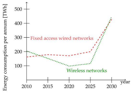
Figure 3.
Estimated annual ICT energy consumption. (Source: data from [4,6]).
Taking into account the fast increase in the energy consumed by networks, it is not surprising that in this area, optimization methods are in use. It should be mentioned, however, that especially in this area, (QoS) and network survivability remain the main goals. The optimization of power usage can affect the robustness to traffic variations in the network, as well as the resilience to the failure of network nodes and links. In [38,39], optimization models are proposed to minimize the energy consumption of Internet Protocol (IP) networks that explicitly guarantee network survivability against failures and robustness to traffic variations.
In the proposed approach, idle line cards and nodes are put in sleep mode in periods of low traffic, thus reducing energy consumption. Two different schemes are used in order to secure network survivability:
- dedicated and shared protection, where a backup path is assigned to each traffic demand;
- leaving spare capacity on the links along the path.
The requested robustness to traffic variations is provided by adjusting the capacity margin on active links in order to accommodate load variations of different sizes. Finally, network stability and device lifetime are secured by additional inter-period constraints.
The model deals with a backbone IP network. Each router consists of a chassis of capacity and a set of line cards each of capacity . Routers are connected by duplex links. It is required that line cards dedicated to link must be available on both routers i and j in order to secure the connectivity of . As a result, the number of operating states of each link depends on the number of line cards powered on. It is assumed that links have the same bandwidth in both directions so the number of powered-on line cards must be the same in both directions. The network can be represented as a symmetric directed graph , where N is the set of chassis and A is the set of bidirectional links and their associated line cards. A positive real parameter denotes the maximum utilization level allowed on each link. This constraint guarantees the required QoS. Consequently, the available bandwidth on a single card is given by . It is assumed that when all line cards connected to a given router are in standby mode, the router chassis can also be put to sleep. The considered time horizon is split into a finite set S of time slots of duration . A set of traffic demands D is considered. Each demand is defined by a source node , a destination node , and the size of demand that has to be fulfilled in period . Let be the positive real parameters representing the hourly power usage of a single card installed on link and the hourly power usage of a chassis. Parameter denotes the additional power usage associated with a chassis switching on. It is assumed that the energy consumption associated with switching on a card is negligible; however, a single-line card cannot be switched on more than times during the day. The goal is to find the routing for each demand and decide which cards and chassis are switched on in each time slot so that the overall energy consumption is minimized. The below mixed integer linear programming formulation for the multi-period energy-aware network management was first presented in [38]. The binary variable is equal to 1 if the path of demand d is routed on link in time slot . Another binary variable is equal to 1 if the chassis i is on in time slot and 0 otherwise. A continuous non-negative variable represents the power usage for switching on chassis j at the beginning of time slot . An integer variable denotes the number of active line cards on link during period . Finally, an auxiliary binary variable represents the number of activations of a card and is equal to one if the k-th card linking nodes i and j is powered on in time slot . The parameter is defined as follows:
The goal is to minimize the total energy consumption in time S (usually one day). The objective function is the sum of three terms corresponding to the energy consumed by the router chassis, the line cards, and the reactivation of the router chassis, respectively:
The problem is known to be NP-complete; the proof uses the reduction from the directed two-commodity integral flow [39]. Additional constraints can be formulated in order to model the resilience and robustness to traffic variations [39]. The computational results show that even high resilience and robustness can guarantee that optimization can bring savings of up to 30% of consumed energy.
In summary, energy consumption can be reduced by switching off some elements of the ICT system when the service demand is lower than the capacity of the system. The objective function is usually the sum of the energy costs and the switching/reactivation cost. This cost is going to be minimized under the constraint that the required quality of service (e.g. response time, resilience, etc.) is guaranteed.
3. Models with Job-Processing Times Depending on Energy Consumption
As follows from Section 1.3 and Section 2, power can be considered a resource influencing the efficiency of computing systems. There is a vast amount of literature on resource-constrained scheduling and it may be interesting to analyze the developments in this field from the point of view of possible applications in energy-aware computing.
3.1. Resource-Constrained Scheduling
In general, scheduling problems are defined as the allocation of resources to jobs for specified amounts of time in order to minimize or maximize a given criterion. Such problems occur in many application areas such as manufacturing, transportation, services, and many others. The optimization of computing systems is one of the traditional fields of application for scheduling models and has inspired a lot of research in this area [40,41].
A classical scheduling problem is defined using three basic elements: a set of jobs, a set of machines, and a set of optimization criteria. Jobs are characterized by their processing times, request of resources, and precedence relationships. A set of machines may contain just a single machine or a number of parallel (identical, uniform, or unrelated) or dedicated machines (flow shop, job shop, or open shop). It is worth mentioning that the vast majority of results refer to a single optimization criterion. The most common criteria are the makespan (schedule length) and mean flow time (average of completion times of jobs). An exhaustive classification of scheduling problems can be found in [40].
Basically, each job requires a machine to be processed. In some situations, however, an additional resource is required to process the job. Moreover, the processing rate/time depends on the amount of the additional resource allocated to the job.
Three basic resource categories are distinguished: renewable, nonrenewable, and doubly constrained resources [42,43,44]. A resource is renewable only if its total usage at every moment is constrained. As soon as a job completes, the resource can be assigned to another job. A resource is nonrenewable only if its total consumption is limited. This means that the units of a nonrenewable resource are consumed by a job during its processing and cannot be assigned to any other job. A doubly constrained resource is a resource whose both total usage at every moment and total consumption over the period of time are constrained.
A resource is called preemptable [45] if each of its units can be preempted. This means that a resource can be withdrawn from the processing of a current job, allotted to another job, and then returned to the previously interrupted job whose processing can be resumed without additional cost. Resources not possessing this property are called nonpreemptable.
From the point of view of divisibility, two categories of resources can be distinguished [46] discrete resources and continuous resources. A discrete resource can be allotted to a job in discrete units from a given finite set of possible allocations, whereas a continuous resource can be allocated in arbitrary amounts from a given interval in .
In the case of discrete resources, reductions between scheduling problems with respect to resource constraints are illustrated in Figure 4 [40].
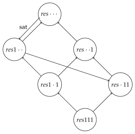
Figure 4.
Polynomial transformations among resource-constrained scheduling problems.
The notation , where , denotes, respectively, the number of resource types, resource limits, and resource requirements. If , then the values are arbitrary, otherwise denotes the number of resource types, maximum number of units available, and maximum job requirements, respectively.
We present further analysis from the point of view of the last classification, showing that continuous and discrete job models lead to significantly different solution approaches and techniques.
Definitions of some other categories of resources not relevant to this survey can be found in [47], where an exhaustive list of resource classifications is provided.
The analysis presented in Section 2 allows us to conclude that power can be modeled as a resource in any of the above categories. Let us recall that power used by a processor at each time unit is limited by the maximum processor frequency so from this point of view, it is a renewable resource. At the same time, the total usage of power over a given horizon (i.e., energy consumption) reflects the “energetic” cost of the schedule and, in some models, can also be limited. The latter perspective corresponds to the definition of a nonrenewable resource. If both conditions are considered in the same model, power is addressed as a doubly constrained resource.
3.2. Modeling Power as a Continuous Resource
One of the most generic job models was proposed by Burkov [48]. This model was first studied in the context of project and machine scheduling by Węglarz [46].
A set of n jobs and m identical machines is considered. Let us denote by the size of job and by the amount of the continuous resource allotted to job i at time , where is the scheduling horizon. We assume that the processing speed of job i is a continuous nondecreasing function of . Without a loss of generality, we can assume that . The current state of job i is denoted by and we express the above relationship as follows:
Further, we formulate the condition guaranteeing that a job will be completed by some (unknown in advance) time :
A solution consists of a sequence of jobs on machines and a vector of continuous resource allocation , which minimizes the makespan, . The continuous resource allocation is a piece-wise continuous, non-negative function of t whose values correspond to the minimum value of M. An important result that holds for is used to obtain the general solution approach. This result states that the minimum makespan as a function of final states of jobs, , can always be given by , where is the convex hull of . M is always a convex function [49]. In the case of concave functions , we can conclude that the makespan is minimized by the fully parallel processing of all jobs using the following resource amounts:
where is the (unique) positive root of the equation
The general solution methodology for the case consists of two steps. In the first step, a sequence of job combinations is created and in the second step, a resource allocation that is optimal for this sequence is found by solving a nonlinear continuous optimization problem. The sequence of job combinations is created based on the observation that each feasible schedule can be divided into intervals defined by the completion times of consecutive jobs. It can be proved [50] that in a makespan optimal schedule and concave functions , each interval contains exactly m jobs. Any feasible schedule is thus represented by a sequence of m-element combinations of jobs such that each job occurs in at least one combination and any two combinations containing the same job cannot be separated by another combination. An example of a feasible schedule with a corresponding sequence of combinations is presented in Figure 5. Notice that the sequence of combinations defines an assignment of jobs to machines and a sequence of job completion times (implying the sequence of jobs on each machine). The completion times of jobs that are optimal for a given sequence are found by solving the nonlinear optimization problems in (22)–(26). A portion of the processing demand of job i completed in interval is a decision variable in the problems in (22)–(26) and is denoted by .
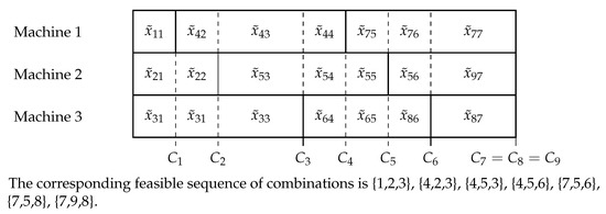
Figure 5.
The idea of discrete-continuous scheduling: a division of the processing demands of jobs.
The objective is to minimize the makespan, i.e., the sum of all intervals. Constraint (23) explicitly uses the results of (21), guaranteeing the minimal length of interval k, whereas Constraint (24) guarantees that all demands will be completed. The resource limit is provided by Constraint (25) and Constraint (26), except for the non-negativity of the variables .
Although we can find an optimal resource allocation for a given sequence of combinations using known analytic or numerical methods, finding the best sequence of combinations remains difficult. The most common approach is to search the space of the feasible sequences using metaheuristic algorithms.
The presented model is very general and does not address any particular resources. It is natural, however, to examine the model in systems where power is the continuous resource influencing the speed of executing a job. The main issue is to define functions . A very common model is that the dynamic power is a function of the speed , where is some constant strictly bigger than 1 [8,51]. It is easy to observe that this model can be considered a special case of Model (19), where
For the function f being a power function, some general properties of makespan optimal schedules have been proved [52]. A very useful one states that if , then Problems (22)–(26) can be solved analytically.
Model (18) was first applied to analyze scheduling jobs in computing systems with limited power availability in [53]. Power was considered a continuous renewable resource. Further, the idea was developed and a more realistic model of power as a doubly constrained resource was formulated in [54].
In [54], the problem of scheduling a set of independent modules of computer programs executed on a multiprocessor portable device with processors driven by a common energy source, e.g., a battery with limited capacity, was considered. The overheating of the computer system was prevented by setting a power limit that respected the data sheet of a processor. Moreover, it was assumed that jobs were preemptable, meaning that any delays related to moving a job to a different processor or changing the amount of resources allocated to a job during its execution were considered negligible. In the proposed model, power is again a doubly constrained resource and the job-processing speed is defined by Equation (27). Release date and deadline are associated with each job. The problem is analyzed from two perspectives. The first problem is formulated as a decision problem with the goal of finding a schedule within the given power limits where all jobs are completed before their deadlines (if such a schedule exists). In the second formulation, the objective is to minimize the power level, guaranteeing the existence of a schedule that respects the deadlines. Some properties of optimal solutions for special cases with identical release dates or deadlines are proved.
The problem studied in [55] is the problem of makespan minimization with and without precedence relationships between jobs. Power is considered a doubly constrained resource, meaning that in addition to Constraint (25) with P interpreted as the amount of power available in each time unit t, the resource allocations must fulfill Constraint (28)
where E is a parameter representing the total amount of energy available to complete the jobs. The precedence relationships are represented by a task-on-arc graph. Such a graph defines an ordering of nodes that, in turn, allows the space of the feasible sequences of job combinations to be restricted. Since even the restricted space is too large for explicit enumeration, some heuristics are proposed to find the orderings of nodes leading to possibly good solutions.
Another issue in energy-aware systems is battery charging. It is worth mentioning here because battery charging is often related to ICT devices. In [56], the problem of scheduling n independent nonpreemptable jobs is considered. Each job is characterized by the amount of consumed energy and the power usage function . The initial power usage is a parameter. The power usage function of job i is defined in Equation (29).
is a nondecreasing function and are the start and completion times of job i, respectively. Now, the job model is defined by Equation (30).
where
and
In [56], some results are presented for a special case of Models (30)–(32), where the power usage function is linear for and . It was proved that for an arbitrary sequence leads to an optimal schedule.
The approach based on the job in Model (27) and the methodology presented above are very general and may be used to model other power-aware computing settings.
A special case of scheduling a set of independent jobs on a single machine, where the power usage per unit time is a convex function of the processor speed is presented in [57]. Each job is characterized by its arrival time , deadline , and the required number of CPU cycles . Energy E consumed in interval is equal to
where the processor speed at time t is denoted by and the power used by the unit time is a convex function of the processor speed. Job i is completed in time interval if
where
Obviously, because no more than one job can be processed at time t.
The objective is to minimize E. Some results are shown for function , where , in particular, for .
3.3. Modeling Power as a Discrete Resource
It seems natural to consider power as a continuous resource because intuitively, it can be assigned to a job in amounts of time from a given interval . In practice, however, some technological constraints can limit this assignment to a finite set of possible values.
In order to illustrate such a situation, let us consider the model introduced by Dror et al. in [58]. Let m refueling terminals driven by a common power source (a pump) be used to refuel a given fleet of n boats. The problem is to find a schedule with a minimum makespan for refueling the fleet of boats. The terminals are identical parallel machines. In general, the output of the pump can be assigned to terminals in arbitrary proportions and from that perspective, it can be considered a continuous resource. The model introduced in [58] assumes, however, that possible allocations of the resource are known in advance and equal to , where is the number of terminals in operation at time t. In conclusion, in this model, fuel is considered a renewable, nonpreemptable, and discrete resource. The processing rate of job i is defined as . For a special case where and is a constant, some properties of schedules optimal with respect to the makespan and mean flow time were proved. It is worth mentioning that the same properties were proved in [50] using Model (18), as presented in Section 3.2. The analogy between fuel and power is very straightforward. As we recalled in Section 1.3, the processing speed of a computational task depends on the power used by the processor.
Machine scheduling with additional resources was introduced in [59]. A survey of further developments in parallel machine scheduling problems with nonpreemptable, renewable, and discrete resources was presented in [60]. Only independent jobs were considered. We are interested in models where the processing speed of a job depends on the amount of a single additional resource allocated to the job, e.g., as seen in [61,62,63].
The general conclusion is that the majority of problems in this group are NP-hard but there are some interesting special cases that have been studied in the literature. For example, quite often it is assumed that the assignment of the resource to jobs is constant during the entire job execution (static problem). The allocation of resource to job i is called job-processing mode by analogy to the resource-constrained project-scheduling problem (RCPSP) [47]. Let T denote the time horizon, denote the available amount of resource , and the processing time of job i executed in mode k. A general model with the objective to minimize the makespan was proposed in [61]. The decision variable if job i completes its processing on machine j at time t and is zero otherwise.
Problems (36)–(40) constitute a makespan minimization problem. Constraint (37) guarantees that at most, one job is executed on a single machine in a given time unit. Equation (38) ensures that every job will be completed and Constraint (39) relates to resource availability. The binary values of the decision variables are ensured by Constraint (40). In the case where the only resource is the power, Constraint (39) takes a simpler form:
Naturally, the complexity of the problem grows with the number of resource types.
Finally, let us mention that it may be useful to discretize the continuous resource. In [64], discretization was proposed in the context of project scheduling; however, the same mechanism can be applied in the case of machine scheduling. Discretization is a concept for selecting a finite number L of values such that . If the resource allocation does not change during the job execution, the processing time of activity i for resource allocation l is then calculated as
In this way, L processing modes of job i are defined. Now, the problem with a job model defined by (18) can be solved using the algorithms proposed for the discrete resource scheduling problems discussed above.
In summary, power can be considered a resource influencing the processing speed/time of a job. Depending on the technological conditions, only a finite number of allocations of amounts of power to a job is considered or this amount may take an arbitrary value from a given interval. In the first case, discrete resource-constrained scheduling models are available, whereas in the latter, discrete-continuous scheduling models can be used. Examples of both approaches have been presented.
4. Discussion
In Section 3, we considered job models where the processing speed is related to power usage. We presented two approaches to modeling power, namely as a discrete or continuous resource. Let us now discuss the features of both models.
4.1. Physical Constraints
Although power is a resource that can be allotted in arbitrary amounts from a given interval , available processors offer a finite number of states associated with a given speed due to technology constraints. As a consequence, processor speed is not a continuous variable. Nevertheless, it may be useful to model it as a continuous variable in order to apply the approach described in Section 3.2.
Equation (23) can be solved analytically for function , which, in fact, represents power as a function of the processing speed, which is a cube function as mentioned in Section 2.1. Models (22)–(26) take the following form:
The technique to model a discrete resource as a continuous one in order to benefit from the solution methods developed for the latter case is known in the literature. We have mentioned considering a large number of processors in a data center as a continuous resource [25]. Another example of this type is to consider a large number of memory pages as a continuously divisible resource, as seen in [46].
4.2. Discretization
Even in a situation where the resource can be assigned in arbitrary amounts (from a given interval of real numbers), it might be useful to apply a discrete model, as we presented in Section 3.3.
The above remarks indicate that in optimization models, power can be considered a discrete or continuous resource. The choice influences the solution techniques, and consequently, also the ability to analyze the problem under the changing parameters. Since the goal of mathematical modeling is not only to find an optimal solution but also to examine the system behavior, it is worth being flexible with respect to model selection.
Continuous models are more general and allow a deeper theoretical analysis of the problem, as mentioned in [50]. However, solving discrete-continuous scheduling problems often requires using nonlinear mathematical programming, which is, in general, time consuming. Using discrete variables can lead to more efficient solution methods, as shown in [64].
5. Conclusions
Undeniably, the further economical development of societies depends strongly on the management of energy production and consumption. Recent decades have proven that energy production cannot grow infinitely, and thus the second aspect, energy consumption, becomes even more important. Analyses show that according to global estimates, one of the crucial factors in technological growth, ICT, is responsible for 5% to 9% of total energy consumption. Forecasts have shown that the share of ICT could grow to 20% of total energy consumption by 2030.
Although a lot of effort has been put into improving the efficiency of ICT devices and systems, the total energy consumption in this sector continues to grow. One of the explanations may be the so-called Jevon’s paradox.
Some limitations also result from the desired QoS, which cannot be sacrificed in order to achieve better energy efficiency.
In order to achieve a good balance between efficient energy consumption and quality of service, mathematical modeling has been successfully used. In this paper, we show two main approaches to solving this problem. The first approach, which is much more popular in the literature, assumes switching the devices on and off, depending on the current workload of the system. The optimization objective takes into account the cost of energy consumed by computation and restarting the devices. The second approach assumes that the processing speed/time depends on the amount of energy assigned to the job. In this case, the objective is to minimize the total computational time under the given limited energy consumption.
Although this survey is restricted to CMOS technology, we would like to point out that the new approach, quantum computing, should also be analyzed from the perspective of energy efficiency. Although quantum computers promise to use much less energy than classical ones, this promise is mainly based on the assumption that quantum computers can potentially perform many more calculations at the same time than classical machines. We should mention, however, that much of the power is used by the refrigeration unit that keeps the quantum processor cool. Thus, the power efficiency of quantum computers is an interesting topic. Analogous to the quantum computing advantage threshold that determines when a quantum processing unit (QPU) is more efficient with respect to classical computing hardware in terms of algorithmic complexity, the “green" quantum advantage threshold is defined in [65] and is based on a comparison of the energy efficiency between the two. In the future, it could play a fundamental role in the comparison of quantum and classical hardware. It has been shown that the green quantum advantage threshold mainly depends on:
- the quality of the experimental quantum gates;
- the entanglement generated in the QPU.
In addition, in [66], it is discussed that there is still space for optimization in the implementation of elementary quantum operations. Physical constraints on the best-case scenario of a quantum computer are formulated. On this basis, the maximal energy efficiency of quantum gates is found, as well as the protocol that attains that maximum. In the future, research on the possible applications of the approaches presented in this paper to quantum computing will be analyzed.
Author Contributions
Conceptualization, R.R. and G.W.; methodology, J.J.; investigation, M.N.; resources, J.J., M.N, R.R. and G.W.; writing—original draft preparation, J.J., R.R. and M.N.; writing—review and editing, J.J., R.R. and G.W.; project administration, G.W.; funding acquisition, R.R. All authors have read and agreed to the published version of the manuscript.
Funding
This research was funded by Poznan Univeristy of Technology grant number 0311/SBAD/0708.
Data Availability Statement
Not applicable.
Conflicts of Interest
The authors declare no conflict of interest.
References
- Yan, Z.; Shi, R.; Yang, Z. ICT Development and Sustainable Energy Consumption: A Perspective of Energy Productivity. Sustainability 2018, 10, 2568. [Google Scholar] [CrossRef]
- Wang, L.; Zhu, T. Will the Digital Economy Increase Energy Consumption?—An Analysis Based on the ICT Application Research. Chin. J. Urban Environ. Stud. 2022, 10, 2250001. [Google Scholar] [CrossRef]
- Lange, S.; Santarius, T.; Pohl, J. Digitalization and Energy Consumption. Does ICT Reduce Energy Demand? Ecol. Econ. 2020, 176, 106760. [Google Scholar] [CrossRef]
- Andrae, A.S. New perspectives on internet electricity use in 2030. Eng. Appl. Sci. Lett. 2020, 3, 19–31. [Google Scholar] [CrossRef]
- Lorincz, J.; Capone, A.; Wu, J. Greener, Energy-Efficient and Sustainable Networks: State-Of-The-Art and New Trends. Sensors 2019, 19, 4864. [Google Scholar] [CrossRef] [PubMed]
- Andrae, A.S.G.; Edler, T. On Global Electricity Usage of Communication Technology: Trends to 2030. Challenges 2015, 6, 117–157. [Google Scholar] [CrossRef]
- Nafus, D.; Schooler, E.M.; Burch, K.A. Carbon-Responsive Computing: Changing the Nexus between Energy and Computing. Energies 2021, 14, 6917. [Google Scholar] [CrossRef]
- Pruhs, K. Green Computing Algorithmics. In Computing and Software Science: State of the Art and Perspectives; Springer International Publishing: Cham, Switzerland, 2019; pp. 161–183. [Google Scholar] [CrossRef]
- Fagas, G.; Gallagher, J.P.; Gammaitoni, L.; Paul, D.J. Energy Challenges for ICT. In ICT—Energy Concepts for Energy Efficiency and Sustainability; Fagas, G., Gammaitoni, L., Gallagher, J.P., Paul, D.J., Eds.; IntechOpen: Rijeka, Croatia, 2017; Chapter 1. [Google Scholar] [CrossRef]
- Mudge, T. Power: A First-Class Architectural Design Constraint. Computer 2001, 34, 52–58. [Google Scholar] [CrossRef]
- Lin, M.; Wierman, A.; Andrew, L.L.H.; Thereska, E. Dynamic right-sizing for power-proportional data centers. In Proceedings of the 2011 IEEE INFOCOM, Shanghai, China, 10–15 April 2011; pp. 1098–1106. [Google Scholar] [CrossRef]
- Albers, S.; Moeller, F.; Schmelzer, S. Speed scaling on parallel processors. In Proceedings of the Nineteenth Annual ACM Symposium on Parallel Algorithms and Architectures, San Diego, CA, USA, 9–11 June 2007. [Google Scholar]
- Albers, S. Energy-efficient algorithms. Mag. Commun. ACM 2010, 53, 86–96. [Google Scholar] [CrossRef]
- Witkowski, M.; Oleksiak, A.; Piontek, T.; Węglarz, J. Practical power consumption estimation for real life HPC applications. Future Gener. Comput. Syst. 2013, 29, 208–217. [Google Scholar] [CrossRef]
- Barroso, L.; Hölzle, U. The Datacenter as a Computer, An Introduction to the Design of Warehouse-Scale Machines. In Synthesis Lectures on Computer Architecture; Hill, M., Ed.; Morgan Claypol Publishers: Williston, VT, USA, 2009. [Google Scholar]
- Bunde, D. Power-aware Scheduling for Makespan and Flow. In Proceedings of the Eighteenth Annual ACM Symposium on Parallelism in Algorithms and Architectures, Cambridge, MA, USA, 30 July–2 August 2006. [Google Scholar]
- Li, K. Energy Efficient Scheduling of Parallel Tasks on Multiprocessor Computers. J. Supercomput. 2012, 60, 223–247. [Google Scholar] [CrossRef]
- Bourhnane, S.; Abid, M.; Zine-dine, K.; El Kamoun, N.; Benhaddou, D. High-Performance Computing: A Cost Effective and Energy Efficient Approach. Adv. Sci. Technol. Eng. Syst. J. 2020, 5, 1598–1608. [Google Scholar] [CrossRef]
- Kormilicin, N.V.; Zhuravlev, A.M.; Khayatov, E.S. Estimation of energy saving in electric drives of traction-blowing mechanisms. In Proceedings of the 2018 17th International Ural Conference on AC Electric Drives (ACED), Ekaterinburg, Russia, 26–30 March 2018; pp. 1–5. [Google Scholar] [CrossRef]
- Gonzalez, R.; Gordon, B.; Horowitz, R. Supply and Threshold Voltage Scaling for Low Power CMOS. IEEE JSSC 1997, 32, 1210–1216. [Google Scholar] [CrossRef]
- Zhuravlev, S.; Saez, J.C.; Blagodurov, S.; Fedorova, A.; Prieto, M. Survey of Energy-Cognizant Scheduling Techniques. IEEE Trans. Parallel Distrib. Syst. 2013, 24, 1447–1464. [Google Scholar] [CrossRef]
- Pering, T.; Burd, T.; Brodersen, R. Voltage scheduling in the IpARM Microprocessor system. In Proceedings of the 2000 International Symposium on Low Power Electronics and Design, Rapallo, Italy, 26–27 July 2000. [Google Scholar]
- Burd, T.D.; Brodersen, R.W. Energy Efficient CMOS Microprocessor Design. In Proceedings of the Twenty-Eighth Annual Hawaii International Conference on System Sciences, Wailea, HI, USA, 3–6 January 1995. [Google Scholar]
- Barroso, L.; Hölzle, U. The case for energy- proportional computing. Computer 2007, 40, 33–37. [Google Scholar] [CrossRef]
- Lin, M.; Wiermn, A.; Andrew, L.; Thereska, E. Dynamic right-sizing for power-proportional data centers. IEEE/ACM Trans. Netw. 2013, 21, 1378–1391. [Google Scholar] [CrossRef]
- Urgaonkar, R.; Kozat, J.; Igarashi, K.; Neely, M. Dynamic resource allocation and power management in virtualized data centers. In Proceedings of the 2010 IEEE Network Operations and Management Symposium—NOMS 2010, Osaka, Japan, 19–23 April 2010. [Google Scholar]
- Bansal, N.; Gupta, A.; Krishnaswamy, R.; Pruhs, K.; Schewior, K.; Stein, C. A 2-competitive algorithm for online convex optimization with switching costs. In Proceedings of the Workshop on Approximation Algorithms for Combinatorial Optimization Problems, Princeton, NJ, USA, 24–26 August 2015. [Google Scholar]
- Chrobak, M.; Dürr, C.; Hurand, M.; Robert, J. Algorithms for temperature-aware task scheduling in microprocessor systems. In Proceedings of the 4th International Conference on Algorithmic Aspects in Information and Management (AAIM’08), Shanghai, China, 23–25 June 2008. [Google Scholar]
- Bampis, E.; Letsios, D.; Lucarelli, G.; Markakis, E.; Milis, I. On multiprocessor temperature-aware scheduling problems. J. Sched. 2013, 16, 529–538. [Google Scholar] [CrossRef][Green Version]
- Birks, M.; Fung, S. Temperature aware online scheduling with a low cooling factor. In Proceedings of the 7th Annual COnference on Theory and Applications of Models of Computation (TAMC’10), Prague, Czech Republic, 7–11 June 2010. [Google Scholar]
- Xiang, Z.; Zheng, Y.; He, M.; Shi, L.; Wang, D.; Deng, S.; Zheng, Z. Energy-effective artificial internet-of-things application deployment in edge-cloud systems. Peer-Netw. Appl. 2022, 15, 1029–1044. [Google Scholar] [CrossRef]
- Vashisht, P.; Kumar, V. A Cost Effective and Energy Efficient Algorithm for Cloud Computing. Int. J. Math. Eng. Manag. Sci. 2022, 7, 681–696. [Google Scholar] [CrossRef]
- Yin, G.; Chen, R.; Zhang, Y. Effective task offloading heuristics for minimizing energy consumption in edge computing. In Proceedings of the 2022 IEEE International Conferences on Internet of Things (iThings) and IEEE Green Computing & Communications (GreenCom) and IEEE Cyber, Physical & Social Computing (CPSCom) and IEEE Smart Data (SmartData) and IEEE Congress on Cybermatics (Cybermatics), Espoo, Finland, 22–25 August 2022; pp. 243–249. [Google Scholar] [CrossRef]
- Zhu, Y.; Halpern, M.; Janapa Reddi, V. The Role of the Mobile CPU in Energy-Efficient Mobile Web Browsing. IEEE Micro 2015, 35, 26–33. [Google Scholar] [CrossRef]
- Corcoran, P.M. Cloud Computing and Consumer Electronics: A Perfect Match or a Hidden Storm? [Soapbox]. IEEE Consum. Electron. Mag. 2012, 1, 14–19. [Google Scholar] [CrossRef]
- Alcott, B. Jevons’ paradox. Ecol. Econ. 2005, 44, 9–21. [Google Scholar] [CrossRef]
- Mastelic, T.; Oleksiak, A.; Claussen, H.; Brandic, I.; Pierson, J.M.; Vasilakos, A. Cloud Computing: Survey on Energy Efficiency. ACM Comput. Surv. 2014, 47, 1–36. [Google Scholar] [CrossRef]
- Addis, B.; Capone, A.; Carello, G.; Gianoli, L.; Sansò, B. Energy management through optimized routing and device powering for greener communication networks. IEEE/ACM Trans. Netw. 2014, 22, 313–325. [Google Scholar] [CrossRef]
- Addis, B.; Capone, A.; Carello, G.; Gianoli, L.; Sansò, B. On the energy cost of robustness and resiliency in IP networks. Comput. Netw. 2014, 75, 239–259. [Google Scholar] [CrossRef]
- Błażewicz, J.; Ecker, K.; Pesch, E.; Schmidt, G.; Sterna, M.; Weglarz, J. Handbook on Scheduling; Springer: Berlin/Heidelberg, Germany, 2019. [Google Scholar]
- Leung, J.Y.T. Handbook of Scheduling. Algorithms, Models and Performance Analysis; Chapman&Hall/CRC: Boca Raton, FL, USA, 2004. [Google Scholar]
- Słowiński, R. Two approaches to problems of resource allocation among project activities—A comparative study. J. Oper. Res. Soc. 1980, 31, 711–723. [Google Scholar] [CrossRef]
- Węglarz, J. On certain models of resources allocation problems. Kybernetes 1980, 9, 61–66. [Google Scholar] [CrossRef]
- Węglarz, J. Project scheduling with continuously-divisible, doubly constrained resources. Manag. Sci. 1981, 27, 1040–1052. [Google Scholar] [CrossRef]
- Błażewicz, J.; Cellary, W.; Słowiński, R.; Weglarz, J. Scheduling Under Resource Constraints: Deterministic Models; J.C. Baltzer AG Science Publishers: Basel, Switzerland, 1986. [Google Scholar]
- Węglarz, J. Time-optimal control of resource allocation in a complex of operations framework. IEEE Trans. Syst. Man Cybern. 1976, 6, 783–788. [Google Scholar]
- Węglarz, J.; Józefowska, J.; Mika, M.; Waligóra, G. Project scheduling with finite or infinite number of activity processing modes—A survey. Eur. J. Oper. Res. 2011, 208, 177–205. [Google Scholar] [CrossRef]
- Burkov, V. Optimal project control. In Proceedings of the IV IFAC Congress, Warszawa, Poland, 16–21 June 1969. [Google Scholar]
- Węglarz, J. Modelling and control of dynamic resource allocation project scheduling systems. In Optimization and Control of Dynamic Operational Research Models; Tzafestas, S., Ed.; North Holland: Amsterdam, The Netherlands; New York, NY, USA; Oxford, UK; Tokyo, Japan, 1982; pp. 105–140. [Google Scholar]
- Józefowska, J.; Węglarz, J. On a methodology for discrete±continuous scheduling. Eur. J. Oper. Res. 1998, 107, 338–353. [Google Scholar] [CrossRef]
- Brooks, D.; Bose, P.; Schuster, S.; Jacobson, H.; Kudva, P.; Buyuktosunoglu, A.; Wellman, J.D.; Zyuban, V.; Gupta, M.; Cook, P. Power-aware microarchitecture: Design and modeling challenges for next-generation microprocessors. IEEE Micro 2000, 20, 26–44. [Google Scholar]
- Józefowska, J.; Mika, M.; Różycki, R.; Waligóra, G.; Węglarz, J. Discrete-continuous scheduling to minimize makespan for power processing rates of jobs. Discret. Appl. Math. 1999, 94, 263–285. [Google Scholar] [CrossRef]
- Różycki, R.; Węglarz, J. On job models in power management problems. Bull. Pol. Acad. Sci. Tech. Sci. 2009, 57, 147–151. [Google Scholar] [CrossRef]
- Różycki, R.; Węglarz, J. Power-aware scheduling of preemptable jobs on identical parallel processors to meet deadlines. Eur. J. Oper. Res. 2012, 218, 68–75. [Google Scholar] [CrossRef]
- Różycki, R.; Węglarz, J. Power-aware scheduling of preemptable jobs on identical parallel processor to minimize makespan. Ann. Oper. Res. 2014, 213, 235–252. [Google Scholar] [CrossRef]
- Różycki, R.; Waligóra, G. Scheduling identical jobs with linear resource usage profile to minimize schedule length. In Proceedings of the 24th International Conference on Methods and Models in Automation and Robotics, Miedzyzdroje, Poland, 26–29 August 2019. [Google Scholar]
- Yao, F.; Demers, A.; Shenker, S. A scheduling model for reduced cpu energy. In Proceedings of the IEEE Symposium on Foundations of Computer Science, Milwaukee, WI, USA, 23–25 October 1995. [Google Scholar]
- Dror, M.; Stern, H.; Lenstra, J. Parallel machine scheduling with processing rates dependent on number of jobs in operation. Manag. Sci. 1987, 33, 1001–1009. [Google Scholar] [CrossRef]
- Błażewicz, J.; Lenstra, J.; Rinnooy-Kan, A. Scheduling subject to resource constraints: Classification and complexity. Discret. Appl. Math. 1983, 5, 11–24. [Google Scholar] [CrossRef]
- Edis, E.B.; Oguz, C.; Ozkarahan, I. Parallel machine scheduling with additional resources: Notation, classification, models and methods. Eur. J. Oper. Res. 2013, 230, 449–463. [Google Scholar] [CrossRef]
- Daniels, R.L.; Hoopes, B.J.; Mazzola, J.B. Scheduling parellel manufacturing cells with resoure flexibility. Manag. Sci. 1996, 42, 1229–1381. [Google Scholar] [CrossRef]
- Ruiz-Torres, A.; Centeno, G. Scheduling with flexible resources in parallel workcenters to minimize maximumcompletion time. Comput. Oper. Res. 2007, 34, 48–69. [Google Scholar] [CrossRef]
- Sue, L.H.; Lien, C.Y. Scheduling parallel machines with resource dependent processing times. Int. J. Prod. Econ. 2009, 117, 256–266. [Google Scholar] [CrossRef]
- Józefowska, J.; Mika, M.; Różycki, R.; Waligóra, G.; Węglarz, J. Solving the discrete-continuous project scheduling problem via its discretization. Math. Methods Oper. Res. 2000, 52, 489–499. [Google Scholar] [CrossRef]
- Jaschke, D.; Montangero, S. Is quantum computing green? An estimate for an energy-efficiency quantum advantage. arXiv 2022, arXiv:2205.12092. [Google Scholar] [CrossRef]
- Aifer, M.; Deffner, S. From quantum speed limits to energy-efficient quantum gates. New J. Phys. 2022, 24, 055002. [Google Scholar] [CrossRef]
Publisher’s Note: MDPI stays neutral with regard to jurisdictional claims in published maps and institutional affiliations. |
© 2022 by the authors. Licensee MDPI, Basel, Switzerland. This article is an open access article distributed under the terms and conditions of the Creative Commons Attribution (CC BY) license (https://creativecommons.org/licenses/by/4.0/).