Article

Geochemical Modelling of the Fracturing Fluid Transport in Shale Reservoirs

1
Computational Earth Science Group, Los Alamos National Lab, Los Alamos, NM 87545, USA
2
Department of Petroleum Engineering, Texas A&M University, College Station, TX 78412, USA
3
Department of Petroleum Engineering, The University of Oklahoma, Norman, OK 73019, USA
*
Author to whom correspondence should be addressed.
Energies 2022, 15(22), 8557; https://doi.org/10.3390/en15228557
Submission received: 19 October 2022 / Revised: 9 November 2022 / Accepted: 14 November 2022 / Published: 16 November 2022
(This article belongs to the Section H1: Petroleum Engineering)

Abstract

:
Field operations report that at least half of the fracturing fluid used in shale reservoirs is trapped. These trapped fluids can trigger various geochemical interactions. However, the impact of these interactions on well performance is still elusive. We modeled a hydraulic fracture stage where we simulated the initial conditions by injecting the fracturing fluid and shutting the well to allow the fluids to soak into the formation. Our results suggest a positive correlation between the dissolution and precipitation rates and the carbonate content of the rock. In addition, we observed that gas and load recovery are overestimated when geochemical interactions are overlooked. We also observed promising results for sea water as a good alternative fracturing fluid. Moreover, we observed better performance for cases with lower-saline connate water. The reactions of carbonates outweigh the reactions of clays in most cases. Sensitivity analysis suggests that the concentration of SO4, K and Na ions in the fracturing fluid, and the illite and calcite mineral content, along with the reservoir temperature, are the key factors affecting well performance. In conclusion, geochemical interactions should be considered for properly modeling the fate of the fracturing fluids and their impact on well performance.

1. Introduction

The shale boom started by combining the multistage hydraulic fracture technique and horizontal drilling technology [1,2,3]. King [4] reported that the recovery of fracturing fluid in shale reservoirs ranges from 10 to 50% depending on the shale characteristics and operational parameters, as shown in Figure 1. Unfortunately, the trapping mechanisms of the fracturing fluids and their impact on well performance are still elusive [5,6,7,8]. In this study, we consider residual trapping, capillary suction, permeability jail and mineral trapping.
Given the heterogeneity of the shale systems, the fate of the fracturing fluid is a multi-faceted topic [9,10,11]. The salinity contrast between the fracturing fluid and the connate water would induce osmosis flow which will impact the load recovery and the well performance, on load recovery [12]. Considering the capillary suction and the osmosis flow, Fakcharoenphol et al. [13] optimized the shut-in time after the well completion to improve the well performance. In the same vein, Le, Hoang and Mahadevan [14] reported that the capillary suction significantly affects the fracturing fluid redistribution in tight rocks and the gas relative permeability in the invaded zone. On the other hand, Agrawal and Sharma [15] showed that the fracturing fluid might also get trapped in the fractures, affecting the load recovery and well performance. Additionally, Gdanski and Walters [16] studied the impact of fracture conductivity, matrix permeability and shut-in time on load recovery and well performance. They attributed the contradictory observations on best practices for shut-in times to the variation of the relative permeability quality between reservoirs. Furthermore, Mahadevan, Sharma and Yortsos [17] examined the potential of water evaporation as a cleaning mechanism for trapped fluids. However, limited research has focused on the impact of induced geochemical interactions on the fate of the fracturing fluid and the well performance.
The introduction of oxygenated, low-salinity and pH-neutral slick water to a reducing, reactive and heterogeneous system like shale would disturb the system equilibrium. The resulting interactions include geochemical reactions such as aqueous, ion exchange and rate-controlled reactions and physiochemical reactions such as clay swelling [18,19]. Akrad, Miskimins and Prasad [20] experimentally investigated the impact of these interactions on reservoir characteristics, where they reported conductivity and strength loss for various shale samples after exposure to slick water. It is notable that, while the conductivity loss directly affects well performance, formation softening endangers the prolonged production lifetime [21].
Figure 1. Load recovery (%) and fracturing treatment volume (MM Gallon) for the main shale-producing plays in the United States (Adapted from King [22]). Vertical lines with end caps represent the error bars.
Energies 15 08557 g001
Shale has a heterogeneous composition consisting of three mineral groups, carbonates, clays and quartz. While carbonates and clay minerals are considered reactive minerals, quartz is considered non-reactive for a well’s lifetime. We also highlighted the differences between sea water, connate water and slick water in terms of salinity and pH, as shown in Figure 2. The incompatibility between injected water and formation brine stimulates scale deposition, which can severely curtail flow capacity and reservoir performance. In addition, the pH contrast stimulates more geochemical reactions to achieve the lost equilibrium. It is worth noting that sea water salinity has a salinity between slick water and formation brine and a relatively high pH value.
This paper studies the impact of geochemical interactions on the fate of the fracturing fluid and the well performance. We organized the rest of the paper as follows: the methodology section presents the model’s details and the geochemical interactions, the results section discusses the well performance and geochemical interactions in various scenarios, the sensitivity study highlights the key factors, and the conclusions section summarizes the main findings.

2. Methodology

Modeling the geochemical interactions accompanying the fracturing fluid is a computationally intensive task. Therefore, an efficient approach is desirable, which optimizes the computational cost and accuracy. We discuss ours in the following subsections.

2.1. Reservoir Modeling

Field observations suggest complex fracture networks in shale reservoirs which makes direct modeling more challenging. Martin [24] presented an analogy between the traditional fractures and shale fracture networks, as shown in Figure 3. While the traditional planar fractures are sufficient to stimulate conventional wells in sandstones and carbonates, the complex fracture networks are essential to enable economical hydrocarbon production from shale reservoirs. However, the explicit modeling of highly unstructured permeable fractures embedded in an ultra-tight matrix is computationally expensive and prone to numerical error. Fortunately, Cipolla et al. [25] proposed the DK-LS-LRG (dual permeability, logarithmically spaced, and locally refined grid) approach, which efficiently accounts for both the conductivity enhancement and the complexity of the fracture network. This approach models the stimulated reservoir volume (SRV) through a network of perpendicular primary and secondary fractures. Figure 4 presents a comparison between explicit hydraulic fracture (EHF) and SRV using DK-LS-LRG.
We simulated a hydraulic fracture stage using a CMG-GEM-GHG module. Table 1 summarizes the reservoir characteristics. We adopted different relative permeability sets for low- and high-salinity waters, as shown in Figure 5. For more discussions on the main characteristics of low- and high-salinity relative permeability sets, we refer the reader to Webb, Lager and Black [26]. While the relative permeability set of the high-salinity water was adopted from literature on tight reservoirs, the relative permeability set of the low-salinity water was defaulted by CMG based on the cation exchange. The software interpolates relative permeability at each step depending on the estimated ion exchange and the corresponding change in water composition. The initial conditions are mimicked by injecting the fracturing fluid, shutting the well for one month to allow the fluids to soak in, and then starting the production. The implementation of a one-month shut-in period was recommended by Mehana and El-Monier [8] so that both hydrocarbon and slick water recovery are optimized.

2.2. Geochemical Interactions

Nghiem et al. [27] developed a fully coupled geochemical EOS compositional simulator. This simulator was initially developed to model CO2 sequestration in subsurface systems. Various modifications, extensions and additions have been incorporated to properly enable the geochemical modeling. Fortunately, the simulator became capable of modeling the aqueous, rate-controlled and ion exchange reactions. Consequently, it has been used to mechanistically model the impact of low-salinity water flooding on the recovery factor. In this study, we extend the applications of this model to study the impact of the fracturing fluid on well performance.
We considered the ion exchange, aqueous and mineral geochemical interactions. All these interactions are reversible and are controlled by the activity of products and reactants, as shown in reaction (1). However, the geochemical modeling of incompatible waters in heterogeneous porous media entails various permutations to determine the path for the least energy system.
The kinetics of mineral reactions include the chemical equilibrium constant, activation energy and specific surface area. While the equilibrium constant depends on the activity of the products and reactants, the activation energy and specific surface area are mineral-specific characteristics. Table 2 and Table 3 summarize our database which is adopted from [27]. Both quartz and K-feldspar minerals are considered non-reactive minerals at reservoir conditions within the well’s lifetime [28].
The cation exchange capacity represents the total amount of exchangeable cations that can be adsorbed on a negatively charged surface. Consequently, both clay minerals and organic matter are expected to have a higher capacity compared to carbonates and quartz. While the charge of the clay minerals is controlled by the isomorphous substitution, the charge of the organic matter is pH-dependent. Therefore, the composition and pH of fracturing fluid highly affect the stability and the structure of surface-charged minerals.
Note that the exchange reactions could explain the impact of water salinity on the wettability alteration of the reservoir matrix. Given that the lower the water salinity is, the more water-wet the matrix becomes, the impact of water salinity on the end points and curvature of the relative permeability could be estimated. Therefore, the interpolations between the low- and high-salinity relative permeability sets are tied to the cation exchange reactions.
Slick water is water with low concentrations of either friction reducer or linear gel [29]. We adopted the detailed chemical analysis of slick water from King [22]. On the other hand, the salinity and ion concentrations of the connate water are formation-specific properties. The chemical analysis of Haynesville shale connate water and another typical connate water are presented in Table 4. We also included sea water composition to evaluate it as a fracturing fluid alternative.
Table 2. Geochemical Modelling Database [30].
MineralArea (m2/m3)Activation Energy (J/mol)Log Keq (mol/(m2s)) at 25 °C
Kaolinite17,60062,760−13.18
Illite26,40058,620−14
Calcite8841,870−8.79
Dolomite8841,870−9.22
Quartz712887,500−13.9
K-Feldspar17667,830−12
Table 3. Ion Exchange Reactions and Constants [31].
Exchange ReactionsExchange Constant (100 °C)
Ca2+ + 2NaX ⟷ 2Na+ + CaX211.31
Mg2+ + 2NaX ⟷ Na+ + MgX27.25
H+ + NaX ⟷ Na+ + HX10
Table 4. Chemical Analysis of Slick, Connate and Sea Water (ppm) [32].
IonsSlick WaterConnate WaterSea WaterHaynesville
HCO34935412-
Ca++2919,04065026,040
SO4−−53502290-
Mg++3243911101460
Na+8059,49110,35218,400
Cl30102,06018,37971,102
K+984-600310
CO3−−640---
Ba+21---
Fe+21---
B+3120---
Si−42---
Total1944183,73433,393117,312

2.3. Sensitivity Analysis

We performed a sensitivity analysis for the impact of water composition, mineral content and reservoir temperature (13 parameters) on well performance using CMOST (CMG module). We used the design of experiment (DOE), fractional factorial design approach to generate sensitivity scenarios to efficiently explore the uncertainty space [33]. The factorial design reduces the number of simulations needed by allowing several factors to change simultaneously. In addition, it quantifies the effect of each parameter and the interactions between the factors as well. We used a two-level design where a high and a low value are assigned for every parameter. A full fractional factorial design would require 213 (8192 runs). However, a fractional factorial design only required 128 runs. Afterward, we used the analysis of variance (ANOVA) to estimate the parameter impact on the output. ANOVA estimates the total variations as the sum of the squares of the deviation from the mean output. Then, the impact of each parameter is the percentage of the variation of this parameter from the total variations. For more details and discussion on fractional factorial design and ANOVA, we refer the readers to Schepdael, Carlier and Geris [33]. We also used the response surface methodology (RSM) correlates the input parameters with the responses (output) using a proxy model where the original reservoir simulation model is replaced with proxy model of linear or quadratic form.

3. Results

In this section, we first present the impact of geochemical interactions on mineral dissolution and precipitation and on well performance. Then, we report the effects of connate water composition and rock mineralogy on well productivity. After that, we highlight the sensitivity analysis results.

3.1. Mineral Dissolution and Precipitation

The disturbance of the geochemical equilibrium, by introducing slick or sea water, stimulates the geochemical reactions to regain the lost equilibrium. The relative availability of the reactants and the products determines the direction of the reversible geochemical reactions. However, in heterogeneous systems such as porous media, where the chemical equilibrium is the outcome of the various mineral, aqueous and ion exchange reactions, the path to the lowest energy state determines the direction of the reactions. Subsequently, this entails various permutations and arrangements to determine the path to the equilibrium state.
Surprisingly, the load and gas recovery resulting from the implementation of sea water as a fracturing fluid surpasses those from slick water. The detailed dissolution and precipitations reactions are presented in Figure 6. It is evident that a higher reaction rate is reported in the case of sea water injection. While dolomite precipitation and calcite dissolution are observed for slick water, the reverse is reported for the case of sea water. This behavior could be attributed to the availability of the “Ca++” and “Mg++” cations in the sea water compared to the slick water. It is worth noting that negligible reactions are observed for the clay minerals in both cases. The reaction kinetics and thermodynamic characteristics of carbonates explain the higher mineral reactivity detected for carbonates compared to clay minerals [28].
Load and gas recovery results for these cases are shown in Figure 7. The poor load and gas recoveries for slick water might be attributed to its relatively limited mobility compared to sea water. On the other hand, ignoring geochemical coupling results in an overestimation of both gas and load recovery.

3.2. The Impact of Connate Water Composition

Connate water salinity and composition is a formation-specific attribute where various equilibrium reactions between the rock and water change the connate water to a highly saline and dense fluid. Therefore, the longer the water resides or migrates in porous media, the more saline it gets. The salinity of the connate water associated with hydrocarbon accumulation ranges from 20 to more than 300 g/L [34].
According to the simulation results presented in Figure 8a, a dramatic change is observed for the slick water case using the connate water composition of Haynesville compared to the base case discussed in the previous section. While the dolomite dissolution is diminished, the kaolinite dissolution and illite precipitation become more tangible. Additionally, higher cumulative gas recovery is observed for Haynesville, as reported in Figure 9a, for both slick and sea water cases. While the load recovery for the slick water case does not exhibit any dependence on the connate water salinity, as shown in Figure 9b, more recovery is observed for the Haynesville case when sea water is used.
The mineral reactions reported in Figure 8b show similar results to what has been observed for the base case. It is worthwhile mentioning that the relatively lower-saline connate water of Haynesville has stimulated more clay minerals reactions. While the clay content change is in the order of tens in the base case, it is in the order of hundreds in the Haynesville case. In addition, a slight increase is reported in both the calcite dissolution and dolomite precipitation. Contrary to slick water, we observed sudden changes in the mineral content after 200 days of production and around 1250 days. These changes are correlated with the changes in the water production presented in Figure 9. We attribute these changes to the water fluxes coming from the natural fractures and formation matrix as the production progresses. These new water fluxes would disturb the achieved equilibrium in the fracture network and might induce new geochemical interactions.
The salinity contrast between the injected water and connate water is a key factor controlling the geochemical interactions and their impact on well performance. Lower salinity contrast leads to enhanced well performance, as can be seen in the case of Haynesville, which has low-saline connate water compared to the base case. This relatively low-saline connate water would result in a better hydrocarbon mobility, as shown in Figure 5. Consequently, better gas recovery is observed for the Haynesville cases compared to the base cases. In addition, better performance was reported for sea water compared to slick water.

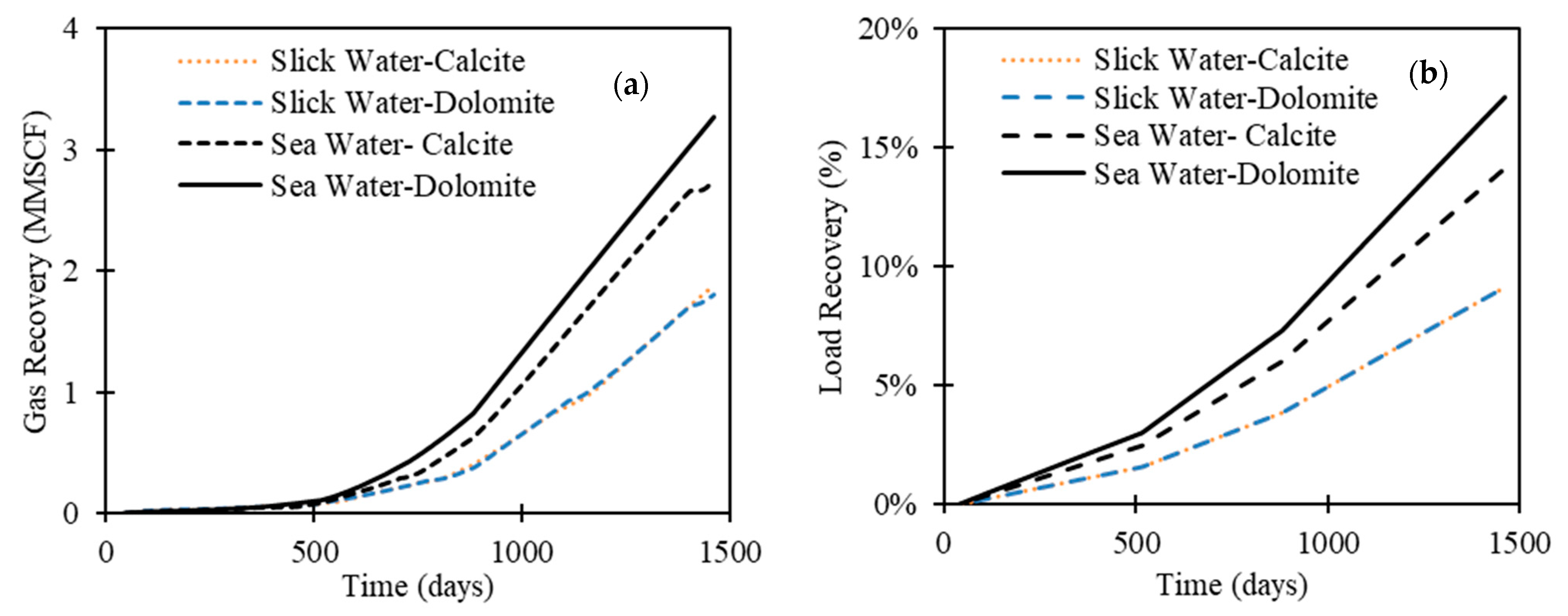
3.3. The Impact of Carbonate Mineral Type

The simulation results suggest that carbonate reactions are more pronounced than clay reactions. Therefore, we discuss the impact of carbonate mineral types on the geochemical reactions and well performance. The main carbonate minerals are calcite (CaCO3) and dolomite (CaMg(CO3)2). While the previous scenarios contained equal mineral content of calcite and dolomite at 15% each, this section involves two cases: one with calcite as the sole carbonate mineral and one with dolomite.
Figure 10 presents the simulation results for the dolomite case. It is evident that the geochemical reactions are depressed when sea water is injected, and subsequently, better gas and load recovery are reported for this scenario in Figure 11 compared to both the calcite case as well as the base case. On the other hand, similar results to the base case are reported for slick water injection when it comes to mineral reactions, as highlighted in Figure 10a.
When dolomite is taken out of the picture, calcite exhibits more reactivity with sea water than slick water, as shown in Figure 12. In the case of slick water, there was no impact on load and gas recovery, as shown in Figure 11. In the case of sea water, the lower reactivity, observed in the dolomite case, results in higher gas and load recovery as shown in Figure 11. In both cases, sea water exhibits better performance compared to slick water. Clearly, slick water is activating the dolomite reactivity, probably due to the absence of Mg+2 ions in the aqueous. On the other hand, sea water activates the dissolution of calcite, where tangible precipitation is observed, leading to lower recovery.

Sensitivity Analysis Results

Shale reservoirs and formations fluids are complex and heterogeneous [35,36,37,38,39]. Therefore, we conducted a sensitivity analysis to identify the key parameters controlling the load and gas recovery. This section presents the sensitivity results of both sea and slick water as fracturing fluid.
The input parameters selected include mineral content, fracturing fluid composition and reservoir characteristics. Table 5 summarizes the upper and lower limit of the input parameters. The total number of simulations is reduced from 213 to 72 by using the DOE and the factorial design options in CMOST. According to the results, a proxy model was generated to emulate the actual reservoir simulation model. In addition, a tornado plot is generated to represent the relative importance of the various factors (the positive effect means a positive correlation between the input parameters and the objective output and vice versa).
According to the sensitivity results for slick water, gas recovery depends mainly on the concentration of K+ and SO 4 2 and illite content, as shown in Figure 13. Equally importantly, load recovery is positively correlated with reservoir temperature and K+ concentration and negatively correlated with SO 4 2 concentration and illite content. On the other hand, the sea water results suggest a positive correlation between both gas and load recovery and the concentration of SO 4 2 and Na+, as shown in Figure 14. In addition, the reservoir temperature enhances the water recovery and lessens the gas recovery in the case of sea water injection.

4. Conclusions

We have investigated the impact of the geochemical interactions on the fate of the fracturing fluid and well performance in shale reservoirs. In addition, we have explored the feasibility of sea water as an alternative fracturing fluid and have provided a sensitivity analysis of the critical factors controlling well performance. The findings support the following conclusions:
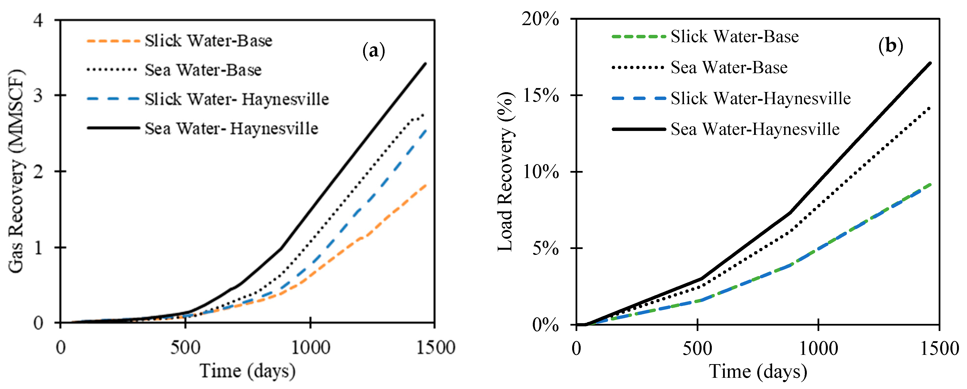
  • Neglecting geochemical coupling results in an overestimation of both load and gas recovery. We observed that geochemical interactions could reduce gas recovery and load recovery by more than 50%.
  • Sea water, as a fracturing fluid, consistently results in higher load and gas recovery compared to slick water (almost double). In fact, the salinity contrast between the injected fluid and the formation brine correlates negatively with well performance. We observed that sea water promotes calcite dissolution, while slick water promotes dolomite dissolution.
  • In most cases studied, clay mineral interactions are minimal compared to carbonate mineral interactions. The highest amount of clay interactions are observed in the case of slick water injection into the lower-salinity connate water case of Haynesville.
  • Sensitivity analysis suggests that the concentration of SO 4 2 , K+ and Na+ ions in the fracturing fluid and illite and calcite mineral content of the rock, along with the reservoir temperature, are the main key factors affecting well performance.
The fate of the fracturing fluids is a puzzling phenomenon. However, geochemical interactions could be responsible for some trapping (more than 50% reduction in the load recovery when considering the geochemical interactions). While computationally intense, geochemical and reactive modeling is sometimes essential for adequately describing the complexity of subsurface phenomena. Coupling reactive modeling and machine learning could alleviate the computational intensity and enable the modeling of more complex systems such as CO2 mineralization.

Author Contributions

Conceptualization, M.M. and M.F.; methodology, M.M.; software, M.M.; validation, M.M. and M.F.; formal analysis, M.M.; investigation, M.M.; resources, M.F., Q.K. and H.V.; data curation, M.M.; writing—original draft preparation, M.M.; writing—review and editing, M.M., M.F., F.C., Q.K. and H.V.; supervision, M.F., Q.K. and H.V.; funding acquisition, M.F., Q.K. and H.V. All authors have read and agreed to the published version of the manuscript.

Funding

This work was supported by the US Department of Energy through the Los Alamos National Laboratory (LANL). LANL is operated by Triad National Security, LLC, for the National Nuclear Security Administration of U.S. Department of Energy (Contract No. 89233218CNA000001). This work was supported by the Laboratory Directed Research and Development program at LANL.

Conflicts of Interest

The authors declare no conflict of interest.

References

  1. Hyman, J.; Jiménez-Martínez, J.; Viswanathan, H.S.; Carey, J.W.; Porter, M.L.; Rougier, E.; Karra, S.; Kang, Q.; Frash, L.; Chen, L.; et al. Understanding hydraulic fracturing: A multi-Scale problem. Philos. Trans. R. Soc. A Math. Phys. Eng. Sci. 2016, 374, 20150426. [Google Scholar] [CrossRef] [PubMed] [Green Version]
  2. Middleton, R.S.; Gupta, R.; Hyman, J.D.; Viswanathan, H.S. The shale gas revolution: Barriers, sustainability, and emerging opportunities. Appl. Energy 2017, 199, 88–95. [Google Scholar] [CrossRef]
  3. Middleton, R.S.; Carey, J.W.; Currier, R.P.; Hyman, J.D.; Kang, Q.; Karra, S.; Jiménez-Martínez, J.; Porter, M.L.; Viswanathan, H.S. Shale gas and non-aqueous fracturing fluids: Opportunities and challenges for supercritical CO2. Appl. Energy 2015, 147, 500–509. [Google Scholar] [CrossRef] [Green Version]
  4. King, G.E. Thirty years of gas shale fracturing: What have we learned? In Proceedings of the SPE Annual Technical Conference and Exhibition, Florence, Italy, 20–22 September 2010. [Google Scholar]
  5. Singh, H. A critical review of water uptake by shales. J. Nat. Gas Sci. Eng. 2016, 34, 751–766. [Google Scholar] [CrossRef] [Green Version]
  6. Hu, Y.; Zhao, C.; Zhao, J.; Wang, Q.; Zhao, J.; Gao, D.; Fu, C. Mechanisms of fracturing fluid spontaneous imbibition behavior in shale reservoir: A review. J. Nat. Gas Sci. Eng. 2020, 82, 103498. [Google Scholar] [CrossRef]
  7. Hun, L.; Bing, Y.; Xixiang, S.; Xinyi, S.; Lifei, D. Fracturing fluid retention in shale gas reservoir from the perspective of pore size based on nuclear magnetic resonance. J. Hydrol. 2021, 601, 126590. [Google Scholar] [CrossRef]
  8. Bai, J.; Wang, G.; Zhu, Q.; Tao, L.; Shi, W. Investigation on Flowback Behavior of Imbibition Fracturing Fluid in Gas–Shale Multiscale Pore Structure. Energies 2022, 15, 7802. [Google Scholar] [CrossRef]
  9. O’Malley, D.; Karra, S.; Currier, R.P.; Makedonska, N.; Hyman, J.D.; Viswanathan, H.S. Where does water go during hydraulic fracturing? Groundwater 2016, 54, 488–497. [Google Scholar] [CrossRef]
  10. Mehana, M.M.; Al, S.; Fahes, M. Impact of salinity and mineralogy on slick water spontaneous imbibition and formation strength in shale. Energy Fuels 2018, 32, 5725–5735. [Google Scholar] [CrossRef]
  11. Mehana, M.M.; Al, S.; Fahes, M. The impact of salinity on water dynamics, hydrocarbon recovery and formation softening in Shale: Experimental study. In Proceedings of the SPE Kingdom of Saudi Arabia Annual Technical Symposium and Exhibition, Dammam, Saudi Arabia, 24–27 April 2017. [Google Scholar]
  12. Mehana, M.; El-Monier, I. Numerical investigation of the osmatic flow impact on the load recovery and early well performance. J. Pet. Eng. Technol. 2015, 5, 52–64. [Google Scholar]
  13. Fakcharoenphol, P.; Torcuk, M.A.; Bertoncello, A.; Kazemi, H.; Wu, Y.-S.; Wallace, J.; Honarpour, M. Managing Shut-in Time to Enhance Gas Flow Rate in Hydraulic Fractured Shale Reservoirs: A Simulation Study. In Proceedings of the SPE Annual Technical Conference and Exhibition, New Orleans, LA, USA, 30 September–2 October 2013. [Google Scholar]
  14. Le, D.H.; Hoang, H.N.; Mahadevan, J. Gas recovery from tight sands: Impact of capillarity. Spe J. 2012, 17, 981–991. [Google Scholar] [CrossRef]
  15. Agrawal, S.; Sharma, M.M. Impact of liquid loading in hydraulic fractures on well productivity. In Proceedings of the SPE Hydraulic Fracturing Technology Conference, The Woodlands, TX, USA, 4–6 February 2013. [Google Scholar]
  16. Gdanski, R.; Walters, H. Impact of fracture conductivity and matrix relative permeability on load recovery. In Proceedings of the SPE Annual Technical Conference and Exhibition, Florence, Italy, 20–22 September 2010. [Google Scholar]
  17. Mahadevan, J.; Sharma, M.M.; Yortsos, Y.C. Evaporative cleanup of water blocks in gas wells. SPE J. 2007, 12, 209–216. [Google Scholar] [CrossRef]
  18. Hajirezaie, S.; Wu, X.; Soltanian, M.R.; Sakha, S. Numerical simulation of mineral precipitation in hydrocarbon reservoirs and wellbores. Fuel 2019, 238, 462–472. [Google Scholar] [CrossRef]
  19. Hajirezaie, S.; Wu, X.; Peters, C.A. Scale formation in porous media and its impact on reservoir performance during water flooding. J. Nat. Gas Sci. Eng. 2017, 39, 188–202. [Google Scholar] [CrossRef]
  20. Akrad, O.; Miskimins, J.; Prasad, M. The effects of fracturing fluids on shale rock mechanical properties and proppant embedment. In Proceedings of the SPE Annual Technical Conference and Exhibition, Denver, CO, USA, 30 October–2 November 2011. [Google Scholar]
  21. Das, P.; Achalpurkar, M.; Pal, O. Impact of formation softening and rock mechanical properties on selection of shale stimulation fluid: Laboratory evaluation. In Proceedings of the SPE/EAGE European Unconventional Resources Conference and Exhibition, Vienna, Austria, 25–27 February 2014. [Google Scholar]
  22. King, G. Fracture Fluid Additive and Formation Degradations. EPA Workshop on Hydraulic Fracturing, Workshop No. 1, Chemicals; 2015. Available online: https://19january2017snapshot.epa.gov/sites/production/files/documents/fracturefluidadditivesandformationdegradations.pdf (accessed on 18 October 2022).
  23. Chermak, J.A.; Schreiber, M.E. Mineralogy and trace element geochemistry of gas shales in the United States: Environmental implications. Int. J. Coal Geol. 2014, 126, 32–44. [Google Scholar] [CrossRef]
  24. Martin, R. Unconventional Completions–A Paradigm Shift–Evening Session; SPE: Dallas, TX, USA, 2015. [Google Scholar]
  25. Cipolla, C.L.; Lolon, E.P.; Erdle, J.C.; Rubin, B. Reservoir Modeling in Shale-Gas Reservoirs. SPE Reserv. Eval. Eng. 2010, 13, 638–653. [Google Scholar] [CrossRef]
  26. Webb, K.; Lager, A.; Black, C. Comparison of high/low salinity water/oil relative permeability. In Proceedings of the International symposium of the society of core analysts, Abu Dhabi, United Arab Emirates, 29 October–2 November 2008. [Google Scholar]
  27. Nghiem, L.; Sammon, P.; Grabenstetter, J.; Ohkuma, H. Modeling CO2 storage in aquifers with a fully-coupled geochemical EOS compositional simulator. In Proceedings of the SPE/DOE symposium on improved oil recovery, Tulsa, OK, USA, 17–21 April 2004; OnePetro: Richardson, TX, USA, 2004. [Google Scholar]
  28. Hakala, J.A.; Vankeuren, A.N.P.; Scheuermann, P.P.; Lopano, C.; Guthrie, G.D. Predicting the potential for mineral scale precipitation in unconventional reservoirs due to fluid-rock and fluid mixing geochemical reactions. Fuel 2021, 284, 118883. [Google Scholar] [CrossRef]
  29. Palisch, T.T.; Vincent, M.C.; Handren, P.J. Slickwater fracturing: Food for thought. In Proceedings of the SPE annual technical conference and exhibition, Denver, CO, USA, 21–24 September 2008. [Google Scholar]
  30. Computer Modelling Group. CMG-GEM Technical Manual; Computer Modelling Group: Calgary, AB, Canada, 2017. [Google Scholar]
  31. Luo, H.; Al-Shalabi, E.W.; Delshad, M.; Panthi, K.; Sepehrnoori, K. A Robust Geochemical Simulator To Model Improved-Oil-Recovery Methods. SPE J. 2016, 21, 55–73. [Google Scholar] [CrossRef]
  32. Fjelde, I.; Asen, S.M.; Omekeh, A. Low salinity water flooding experiments and interpretation by simulations. In Proceedings of the SPE improved oil recovery symposium, Tulsa, OK, USA, 14–18 April 2012. [Google Scholar]
  33. Schepdael, A.V.; Carlier, A.; Geris, L. Sensitivity analysis by design of experiments. In Uncertainty in Biology; Springer: Berlin/Heidelberg, Germany, 2016; pp. 327–366. [Google Scholar]
  34. Shehata, A.M.; Nasr-El-Din, H.A. Reservoir connate water chemical composition variations effect on low-salinity waterflooding. In Proceedings of the Abu Dhabi International Petroleum Exhibition and Conference, Abu Dhabi, United Arab Emirates, 10–13 November 2014. [Google Scholar]
  35. Tang, H.; Li, S.; Zhang, D. The effect of heterogeneity on hydraulic fracturing in shale. J. Pet. Sci. Eng. 2018, 162, 292–308. [Google Scholar] [CrossRef]
  36. Yucel, A.I.; Fathi, E. Multiscale gas transport in shales with local kerogen heterogeneities. SPE J. 2012, 17, 1002–1011. [Google Scholar] [CrossRef] [Green Version]
  37. Fathi, E.; Akkutlu, I.Y. Matrix heterogeneity effects on gas transport and adsorption in coalbed and shale gas reservoirs. Transp. Porous Media 2009, 80, 281–304. [Google Scholar] [CrossRef]
  38. Borrok, D.M.; Yang, W.; Wei, M.; Mokhtari, M. Heterogeneity of the mineralogy and organic content of the Tuscaloosa Marine Shale. Mar. Pet. Geol. 2019, 109, 717–731. [Google Scholar] [CrossRef]
  39. Chen, Y.; Mastalerz, M.; Schimmelmann, A. Heterogeneity of shale documented by micro-FTIR and image analysis. J. Microsc. 2014, 256, 177–189. [Google Scholar] [CrossRef] [PubMed]
Figure 2. Comparison between connate, slick and sea water in terms of salinity and pH [23].
Energies 15 08557 g002
Figure 3. Analog comparison between (a) unconventional fracturing and (b) conventional planar fracture [20].
Energies 15 08557 g003
Figure 4. Schematic illustration of the SRV using (a) DK-LS-LRG and (b) EHF.
Energies 15 08557 g004
Figure 5. Relative permeability sets for low- and high-salinity water.
Energies 15 08557 g005
Figure 6. The mineral content change (gmole): (a) slick water and (b) sea water.
Energies 15 08557 g006
Figure 7. Well Performance: (a) gas recovery, (b) load recovery.
Energies 15 08557 g007
Figure 8. The mineral content change (gmole) using Haynesville connate water composition: (a) slick water and (b) sea water.
Energies 15 08557 g008
Figure 9. Stimulated well performance using Haynesville connate water composition: (a) gas recovery, (b) load recovery.
Energies 15 08557 g009
Figure 10. The mineral content change (gmole) using dolomite as the sole carbonates mineral: (a) slick water and (b) sea water.
Energies 15 08557 g010
Figure 11. Stimulated well performance with calcite and dolomite as the only carbonates minerals: (a) gas recovery and (b) load recovery.
Energies 15 08557 g011
Figure 12. The mineral content change (gmole) using calcite as the sole carbonates mineral: (a) slick water and (b) sea water.
Energies 15 08557 g012
Figure 13. The effect estimates of the main parameters for slick water as fracturing fluid.
Energies 15 08557 g013
Figure 14. The effect estimates of the main parameters for sea water as a fracturing fluid.
Energies 15 08557 g014
Table 1. Input Parameters for Reservoir Simulation.
Model ParametersValue
Model Dimensions420 × 420 × 100 ft.
Reservoir Pressure5000 psi
Matrix Porosity7%
Natural Fracture Porosity1%
Matrix Permeability1.5 × 10−4 md
Fracture Conductivity4.13 md-ft.
Reservoir Temperature250 F
Natural Fracture Spacing10 ft.
Shut-in time1 month
Table 5. The upper and lower limits for the sensitivity analysis input parameters.
ParameterSlick WaterSea Water
BaseLowerUpperBaseLowerUpper
Ca+2 (Mole/L)0.0007240.0005430.0009040.0002990.0002250.000374
Cl (Mole/L)0.0008460.0006350.0010580.51840.38880.648
H+ (Mole/L)9.9216 × 10−77.44 × 10−71.24 × 10−69.92 × 10−117.44 × 10−111.24 × 10⁻¹⁰
HCO−3 (Mole/L)0.016380.012290.02050.010650.0079890.01332
K+ (Mole/L)0.025170.018880.031460.045660.034250.05708
Mg+2 (Mole/L)0.0001239.26 × 10−50.0001540.45670.33770.5629
Na+ (Mole/L)0.003480.0026090.0043490.023840.017880.0298
SO 4 2 (Mole/L)5.21 × 10−53.90 × 10−56.51 × 10−50.0115341.15 × 10−21.92 × 10⁻²
T (F)250187.5312.5250187.5312.5
Calcite0.150.11250.18750.150.11250.1875
Dolomite0.150.11250.18750.150.11250.1875
Illite0.150.11250.18750.150.11250.1875
Kaolinite0.150.11250.18750.150.11250.1875
Publisher’s Note: MDPI stays neutral with regard to jurisdictional claims in published maps and institutional affiliations.

