Abstract
District heating systems (DHS) are driven by the heat demands of their consumers, with higher demands giving a higher load on the heat production. While heat demands are human-dependent, they contain diurnal behaviors and weather dependencies. The diurnal behaviors contain periods with high demands causing peak loads on the heat production, which is operationally costly. This is especially true for heat pumps, a solution for DHS to include green energy, as the cost depends directly on the needed temperature. This paper presents a formulation of adaptive model predictive control (MPC) for inducing peak shaving on the production load to handle the peak load problem by using the DHS distribution network as a heat storage. It also presents a simulator model to describe the DHS. The MPC was applied to data from a case study of the DHS in Brønderslev, Denmark, showing a peak reduction of around .
1. Introduction
The heating consumption of houses, industries, cities, etc., all have diurnal behaviors [1], daily periods where their demand is high and periods where it is low. This results in peak loads on the heat production, where the peak loads are often more expensive to produce due to the higher temperature needs during the peak load as well as the production unit mix used to cover the peak.
District heating systems (DHS) is particularly affected by these peak loads, as the production is far from the consumption, giving a delay between temperature increase and its distribution, inducing higher inflows to fulfill demands, thus raising the supply power and production costs. The importance of this issue is likely to increase as heat pumps are being integrated into DHS as part of the transition to green energy, with their production cost being directly dependent on the needed supply temperature.
A DHS is a network for the distribution of heat to an entire district [2], see Figure 1, utilizing large-scale heat production instead of independent production per consumer, as in the case of gas. DHS is generally controlled through the supply temperature, while the inflows are governed by differential pressure. The heat is distributed through a medium, usually water, using the pipes of the network. While the pipe loses heat to the surroundings, it also stores the water until it reaches the consumer. Given the diurnal nature of the demand, it is possible to forecast when the demand is expected to increase [3].
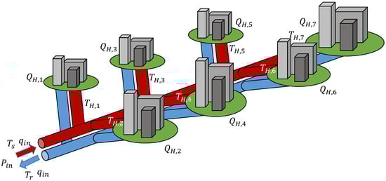
Figure 1.
District heating system—a conceptual layout of how consumers are distributed along the pipes, for .
To ensure that the supply temperature is high enough to satisfy the demand, but not higher than is needed, model predictive control (MPC) methods have previously been utilized, in combination with forecasts of heat demand [4,5]. MPC is a well-studied control method [6,7], capable of dealing with prediction and constraints. It has successfully been applied to multiple fields, such as cement production [8], urban drainage [9], district heating [10], and more [11].
To address the problem of peak load on the production, this paper contributes with the formulation of an MPC design to minimize the peak loads, using the pipe system to store heat energy. The main idea is to use the preheating of the water entering the pipe system prior to the peak load occurring, utilizing the transport delay as an opportunity for heat storage. The stored water in the pipe system then has a higher temperature, from which the coming load can draw power, thus reducing the need for increasing the supply power at the time.
Additionally, a surrogate model for the DHS is formulated and calibrated for the case of the district heating system in Brønderslev, Denmark. Brønderslev is a city of approx. 12,500 people, where the DHS supplies 5000 out of 5500 houses with heating [12]. This model is used to evaluate the proposed controller.
In the following sections, we start with outlining the surrogate model, then the MPC design, and end with the evaluation of the design.
2. Modeling of District Heating
District heating systems consist of a network of pipes. They can in general be considered to consist of two main pipes, one supplying and one returning, and branches with subnetworks as illustrated in Figure 1. The areas in these branches can then be lumped together as single houses, giving a simple lumped model of houses along a pipe.
As the return temperature of each house can be assumed roughly the same, our model assumes the temperature of the return pipe to be the same along the pipe, simplifying the model to a single pipe.
As pipes in district heating are constantly full, we describe the pipe using volume elements in discrete time, such that in each period, the volume leaving the pipe equals the volume entering, as illustrated in Figure 2. Each element is then described by its temperature, volume, and position in the pipe, while being updated as it traverses through the pipe. This gives a discrete description of the stored heat energy and its distribution along the pipe.
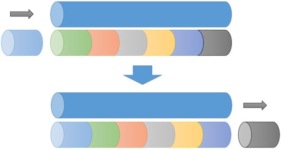
Figure 2.
Element model: the principle of volume elements moving through the pipe system.
The model includes two updates for the elements: (1) the contained volume; as the element passes by houses, flows to the houses are subtracted from the volume by (1). (2) Heat loss to the environment [13]; as an element moves through a pipe section, heat is lost as (2), and illustrated in Figure 3.
where is the return temperature, is the temperature going into the house, is the ground temperature, is the ingoing temperature of the section, and is the inflow to the section. The remaining parameters are the section length , the section depth , the section diameter , the section’s thermal conductivity , the heat loss , the house flow , and the heat demand .
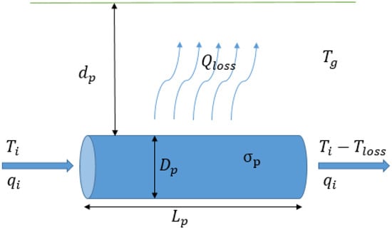
Figure 3.
Pipe heat loss with related parameters and variables.
In district heating, the pipe dimensions decrease along the network; by splitting the pipe model into sections between houses, the dimensions can be represented as seen in Figure 4.

Figure 4.
House junction point—dimension concept of a pipe before and after the connection to a house: change in pipe size.
2.1. Model Dimensioning—Brønderslev
For the particular model discussed in this paper, we utilized data and forecasts from the district heating system in Brønderslev, Denmark. For the dimensioning of said model, we considered the static case, where the flow velocity v is constant throughout the pipe, giving a constant ratio between static flow and cross-area :
The model was calibrated assuming a total temperature loss of 5 °C from the entrance to the last house, a typical value for a Danish DHS during winter operation. For the calibration, the static supply temperature, return temperature, and heat load were determined as the average from the available data.
Additionally, we assumed that the total transport time through the pipe system was 4 h, that there were 10 houses () along the pipe (branches), and that they were equally spaced with equal heat demands. Each pipe section was assumed to have equal temperature loss. With an assumed constant velocity, the transportation time, loss, and pipe temperature of each pipe section are given by:
Assuming each house has equal heat demand, the flows to each house, inflow, and flow through each pipe section are given by:
With the flows, temperatures, and transport times determined, the dimensions of the pipe model can be computed according to the mentioned assumptions.
where and .
2.2. Model Computation
As discussed, the model consisted of a series of volume elements describing the state along the pipe. Each element tracked its current/previous position, its temperature, volume, and its initial temperature when entering the current section.
At each time step, the simulator determined the needed inflow, by computing the heat consumption of the houses based on their demands and the pipe and supply temperatures. A new element was then added to the pipe, filling the pipe volume, while empty ones were removed. The heat loss of each element was then computed based on the element’s translation through the pipe. The details of the consumption and heat loss are discussed in the following parts, where is the sampling time of the discrete model.
2.2.1. Consumption
The consumption of a given house was computed by subtracting the needed volumes from the nearest pipe elements at or upstream of the house. Starting with the house at the end of the pipe, the consumption was computed independently for each house. From each element, only the volume part that was upstream of a house was used. If the positions of the element and the house are given in volume along the pipe, then the available needed volume of the element to fulfill the heat demand of the house is given by
where is the house position, is the back position of the element (upstream end), is the current demand of the house, and and are the volume and temperature of the element, respectively. Correspondingly, the element’s volume and the demand of the house are then reduced:
If the demand is unfulfilled (not zero), the procedure is repeated for the next element upstream of the house. When demand is fulfilled after, e.g., n elements, the flow and temperature supplied to the house for satisfying the demand are given by
The necessary inflow is then obtained after repeating the above computation for each house:
2.2.2. Computations of Losses
The heat loss of the elements can then be determined from the element’s change in position. As each pipe section has different dimensions, the heat losses are computed in parts, starting from the previous position to the nearest passed house , then to the next passed house until the current position is reached.
If is the end of the considered part of section i (the smallest of and ), then the procedure is given by Algorithm 1.
| Algorithm 1 Heat Loss of Element. |
| Require: i = section # of past position |
| while do |
| (1) Determine the moved amount: |
| (2) Compute the time spent and the moved length: |
| (3) Determine the heat loss, where is the temperature when entering that section. |
| (4) Apply the heat loss and update the temperature: |
| (5) Update the positions (past, part and section # i ): |
| end while |
When the heat losses have been applied, then the diffusion between elements can be computed for each element:
where r is the mixing rate (a mixing rate of was used throughout this work), with and being the temperature of the elements up- and downstream of the specific element.
2.2.3. Model Simulations
To test the model, simulations using historical data were used. As flow was computed by the model, we could compare the computed flow to the historical flow to evaluate the model. The used data of the heat demands were from the utility company’s measurements of the overall demand/consumption for the period of the data. In Figure 5, the flow of two simulations (dimensioning with 0 °C and 5 °C of total temperature loss) is given next to the historical flow. It can be seen that the 0 °C simulation is the closest match to the historical data, while the 5 °C induces slightly higher flows. Both simulations occasionally experience negative overshoots, as the approximation using the lumped model diverges from the historical data, due to the sampling time and the size of the elements.
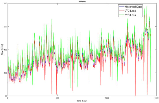
Figure 5.
Historical supply flow (blue) vs. simulated flows for 0 °C (red) and 5 °C loss (green).
As mentioned earlier, the 5 °C of total temperature loss was used in the dimensioning of the model in the later sections; this was chosen to ensure the simulation with MPC would have a temperature loss to consider, given the heat load data of the system included not just the actual heat load of houses but also the heat losses.
3. MPC Design
For the MPC design over a prediction horizon , a dynamic description is needed to describe the relationship between the control variables and the objectives. As this work focused on peak shaving of supply power, we utilized the definition of the supply power as a base for the design:
depending on both the inflow and the supply temperature. The inflow in return relied on the heat demands and the house temperatures throughout the pipe:
and the house temperatures were similarly affected by past loads and operations, thus coupling the supply powers at different times.
3.1. System Identification and Models
In the simulations, we used historical data and forecasts from the DHS in Brønderslev. The available data included the supply temperature, return temperature, and total heat load (losses + demand), as well as forecasts of load and supply temperature. The data and forecasts were provided by ENFOR, using methods for heat load forecasts [3] and supply temperature forecasts [14].
As the data and forecasts described the system externally, and the detailed system described above was highly nonlinear, given the house temperatures’ interconnection, we applied an adaptive approach to keep the design model simple, utilizing system identification (SysId) through the onlineforecasting package in R [15,16]. More specifically, we used recursive fitting [17] to obtain a prediction model based on historical forecasts and data, updating the model parameters when new data were available.
In this work, we tested five model structures for the MPC design, see (16)–(20),
where for the k-step ahead, is the heat load, is an estimate/forecast of the average house temperature, is the parameter for the first-order unit-gain low-pass function , and is the model coefficients determined through the recursive fitting.
The estimate was based on the simple assumption that the supply temperature lost a fixed amount of degrees per house passed, making each house temperature equal to a scaled past supplied temperature:
Each model and its motivation can be summarized as: (1) Model 1 approximates the physical structure of the system. (2) Model 2 is simplified but preserves the multiplicative structure. (3) Model 3 adds more degrees of freedom to model 2. (4) Model 4 is simplified but approximates the fractional structures. (5) Model 5 is the simpler linear model.
From the above discussion, we can see that all of our models take the same general low-pass form, see (22). For the k-step, the low-pass form can be rewritten to a linear form with respect to the control variables on the form:
where is the control variables, , , and are the remaining variables inside the low-pass filter of (16)–(20), and is a scaling variable on the low-pass filter. n is the number of terms in the model. Now, let and be the matrix and vector describing the entire power prediction:
giving the models a linear description over the prediction horizon with regard to the control variables.
3.2. Cost and Objectives
With the models defined, the MPC design can be addressed. The main part of the design was the definition of the optimum through the objectives in the cost function. The objectives were (1) inducing peak shaving through the reference-tracking of the power, (2) keeping the supply temperature low for the production cost, (3) keeping the production steady, through a minimum variation of the supply temperature. The objectives were all given as quadratic costs:
where is the power reference, defined as the mean forecasted power within the horizon:
The idea behind the first objective was to shift the top of the supply peaks to periods where the load from heat demand was below the reference, essentially averaging out the loads. Physically, this is done by storing up heat energy in the pipe system; the flow then distributes the heat along the pipe to be ready, increasing the temperature before higher demands occur. Applying the model structures, the cost function can be written as:
The MPC based on each model was tuned visually to induce peak shaving. The tuned weights can be observed in Table 1.

Table 1.
The visual tuned weights of each control design.
3.3. Constraints
The second part of MPC design is the constraints. For these controllers, the operational limits of the supply temperature regarding the temperature and its change were formulated as the constraints of the MPC:
where the minimum supply temperature was chosen as the forecasted supply temperature, to ensure a guaranteed base performance of the system. The maximum supply temperature was chosen as 85 °C, while the change limits were chosen as a 5 °C limit.
The constraints can be expressed purely in terms of the supply temperatures (no change) as
where is the past supply temperature.
4. Results
To evaluate the designed MPCs and the approach to peak shaving, we used simulations based on the model discussed in Section 2, using demand and data from a historical scenario. Each model case was given the exact same scenario and data: an initial 70-day data set for initializing the model spanning 1 March 2021 to 9 May 2021, then simulating the adaptive MPC over a period of 10 days, 10 May 2021 to 19 May 2021. For comparison, a base simulation was performed using the historical inputs and the system model. As the data were given in 1 h increments, the simulation and MPCs utilized a 1 h sampling time as well. The used data on the demands had a trend with the highest loads between 5 to 9 AM, with another small high around 18 to 19. The daily variation was around 0.4 MW, see Table 2.
Table 2.
Demand trends: the hourly trends of the heat demand, showing the mean, standard variation, minimum, and maximum values for each hour in MW.
4.1. Visual Evaluation
In Figure 6, Figure 7, Figure 8, Figure 9 and Figure 10, the performance of the MPCs is shown alongside historical and/or base simulation performance, each figure consisting of four graphs: (1) The top graph illustrates the supply and return temperatures evolution over time, both simulated, forecasted, and historical supply temperature is displayed. (2) The inflow over time is shown in the top-middle graph for the historical inflow, and the simulations of the MPC and the baseline. (3) The bottom-middle graph displays the supply power of the simulations, as well as the utilized historical load of the system. (4) The bottom graph shows how the stored energy in the system changes over time, for the simulations with the MPC and the baseline.

Figure 6.
Performance results of model 1, showing peak shaving through heat storing. MPC results (red), base simulation (blue), and historic results (green).
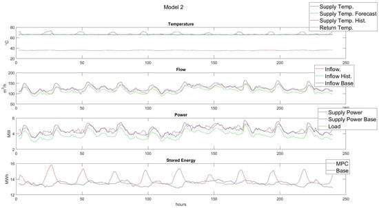
Figure 7.
Performance results of model 2, inducing peak shaving with increases in stored energy. MPC results (red), base simulation (blue), and historic results (green).
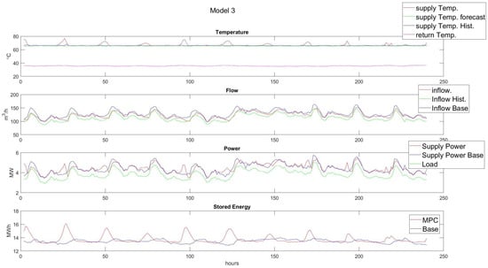
Figure 8.
Performance results of model 3, showing peak shaving though also inducing large peaks. MPC results (red), base simulation (blue), and historic results (green).
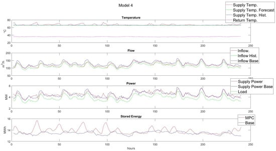
Figure 9.
Performance results of model 4, inducing peak shaving but also inducing large peaks. MPC results (red), base simulation (blue), and historic results (green).
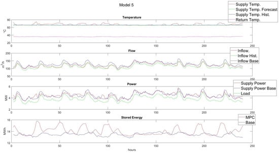
Figure 10.
Performance results of model 5, inducing peak shaving, though with an increase in supply temperature. MPC results (red), base simulation (blue), and historic results (green).
Model 1’s performance is shown in Figure 6. We can observe the supply temperature only diverges from the forecast in order to charge the system with stored energy, temporally increasing supply power. These charging periods happen prior to the peak loads occurring, resulting in the following power peak being reduced/shaved in comparison to the base. Importantly, the new peaks from the charged power are significantly smaller than the base supply peaks. A similar reduction and behavior are seen in the flow.
In Figure 7, the performance of model 2 is shown. It performs similarly to model 1 with an increased supply temperature for storing heat energy in the pipe system, though the amount of shaving is larger for model 2.
Furthermore, model 3 also has a similar performance to model 1, as seen in Figure 8, the general difference being a higher size of the charged power peaks than in model 3, occasionally comparable to the base supply peaks.
In model 4’s case, shown in Figure 9, the charging of the system can be observed, though the peak shaving occurs only occasionally. The charging time with a higher supply temperature also tends to be longer.
The performance of model 5 is shown in Figure 10, showing peak shaving, with substantially longer charging periods, extending into the peak period.
Given the visual performances of the MPCs, model 2 would be the MPC design which performed best. The high-induced supply power peaks excluded model 3 and 4 as the new peaks ran counter to the purpose of peak shaving. Model 5 was likewise unsuitable as its long period of charging indicated higher production costs. Between models 1 and 2, model 2 was preferable with its slightly larger peak shaving.
4.2. KPI-Based Evaluation
Key performance indexes (KPI) can reduce performance to a few numbers. In this evaluation, we focused on the following list of KPIs, with each model’s KPI shown in Table 3.
Table 3.
KPI results for the simulation of the five models.
- Added temperature: the average amount of degrees added to the supply temperature, in comparison to the forecast.
- Added energy: the additional energy applied to the entrance of the system
- Shaved peak power: the average difference of max peak powers at each event between base and MPC. Each event lies within a 12 h interval (12 AM–12 PM or 12 PM–12 AM).
- One-sided: only model peaks in the interval occurring prior to the maximum base peak are considered
- Two-sided: all model peaks in the interval are considered.
Since the performance of models 1–3 were relatively similar, the best model then depended on the importance given to each KPI. The increase in energy consumption was fairly even around 0.6%. Models 1 and 3 performed better keeping the temperature low, while model 2 was better at peak shaving. Overall, model 2 was the best performer when prioritizing peak shaving, with its 0.43 MW average reduction, roughly of the general power peak or for the two-sided peak shaving.
The overall KPI results show the best results were from the models preserving the multiplicative structure, models 1, 2, and 3, outperforming models 4 and 5 in every KPI.
Based on both the KPI and the visual analysis, model 2 was the best choice for a design model, with model 1 being a close alternative, providing a trade-off between peak shaving and low-temperature importance.
5. Conclusions
In this paper, we proposed formulations of adaptive model predictive control (MPC) for handling the peak load problem of supply power in district heating, through pipe energy storage. A model was similarly presented, for the purpose of simulating district heating systems approximated as a single pipe with distributed loads.
Several MPC formulation designs were proposed and applied to a case study of the district heating system in Brønderslev, Denmark. It was found that a simple physics-inspired model, named model 2, had the best performance among the designs, providing around of peak shaving in supply power without inducing unwarranted behaviors, such as new large power peaks.
Future Work
A continuation of the work could include a real-world application to an actual district heating system (DHS) or application to data from other DHS than the Brønderslev case. As model 1 was close to model 2 in performance, an updated design description of the house temperatures or the inclusion of internal pipe temperature measurements in the design could be added.
Funding
This research was funded by Innovation Fond Denmark through the FED project (project 8090-00069B), the TOP-UP project (project 9045-00017A), and the Heat 4.0 project (project 8090-00046B).
Data Availability Statement
Restrictions apply for the availability of these data. Data were obtained from ENFOR A/S and are available through and with the permission of ENFOR A/S.
Acknowledgments
I would like to thank ENFOR A/S and especially Torben Skov Nielsen for providing access to the necessary data, insights into district heating, cooperation, and discussions during the project period.
Conflicts of Interest
The funders had no role in the design of the study; in the collection, analyses, or interpretation of data; in the writing of the manuscript; or in the decision to publish the results.
Abbreviations
The following abbreviations are used in this manuscript:
| DHS | District heating system |
| MPC | Model predictive control |
References
- Gadd, H.; Werner, S. Daily heat load variations in Swedish district heating systems. Appl. Energy 2013, 106, 47–55. [Google Scholar] [CrossRef]
- Lund, H.; Werner, S.; Wiltshire, R.; Svendsen, S.; Thorsen, J.E.; Hvelplund, F.; Mathiesen, B.V. 4th Generation District Heating (4GDH): Integrating smart thermal grids into future sustainable energy systems. Energy 2014, 68, 1–11. [Google Scholar] [CrossRef]
- Nielsen, H.A.; Madsen, H. Predicting the Heat Consumption in District Heating Systems Using Meteorological Forecasts; Technical Report; IMM, DTU: Kongens Lyngby, Denmark, 2000. [Google Scholar]
- Nielsen, T.; Madsen, H. Control of Supply Temperature in District Heating Systems. In Proceedings of the 8th International Symposium on District heating and Cooling, Trondheim, Norway, 14–16 August 2002. [Google Scholar]
- Bavière, R.; Vallée, M. Optimal Temperature Control of Large Scale District Heating Networks. Energy Procedia 2018, 149, 69–78. [Google Scholar] [CrossRef]
- Propoi, A. Use of LP Methods for Synthesizing Sampled-data Automatic Systems. Autom. Remote Control 1963, 24, 837–844. [Google Scholar]
- Kouvaritakis, B.; Cannon, M. Model Predictive Control—Classical, Robust and Stochastic; Advances Textbooks in Control and Signal Processing; Springer: Cham, Switzerland, 2016. [Google Scholar] [CrossRef]
- Prasath, G.; Recke, B.; Chidambaram, M.; Jørgensen, J. Application of Soft Constrained MPC to a Cement Mill Circuit. In Proceedings of the 9th International Symposium on Dynamics and Control of Process Systems, Leuven, Belgium, 5–7 July 2010; pp. 288–293. [Google Scholar]
- Svensen, J.L.; Sun, C.; Cembrano, G.; Puig, V. Chance-constrained Stochastic MPC of Astlingen Urban Drainage Benchmark Network. Control Eng. Pract. 2021, 115, 104900. [Google Scholar] [CrossRef]
- Hermansen, R.; Smith, K.; Thorsen, J.; Wang, J.; Zong, Y. Model predictive control for a heat booster substation in ultra low temperature district heating systems. Energy 2022, 238, 121631. [Google Scholar] [CrossRef]
- Qin, S.J.; Badgwell, T.A. A survey of industrial model predictive control technology. Control Eng. Pract. 2003, 11, 733–764. [Google Scholar] [CrossRef]
- The Organization of Brønderslev Forsyning. Available online: https://bronderslevforsyning.dk/organisation/organisationen/datterselskaber/ (accessed on 7 November 2022).
- Çengel, Y. Heat Transfer: A Practical Approach; McGraw-Hill Series in Mechanical Engineering; McGraw-Hill: New York, NY, USA, 2002. [Google Scholar]
- Nielsen, T.S. Online Prediction and Control in Nonlinear Stochastic Systems. Ph.D. Thesis, DTU, Kongens Lyngby, Denmark, 2002. [Google Scholar]
- Onlineforecast: An Adaptive Forecasting Package in R. Available online: https://onlineforecasting.org/ (accessed on 13 September 2022).
- Barcher, P. Description of the Onlineforecast R Package; Technical Report; DTU Compute: Kongens Lyngby, Denmark, 2019. [Google Scholar]
- Madsen, H. Time Series Analysis, 3rd ed.; Chapman & Hall/CRC: Boca Raton, FL, USA, 2007. [Google Scholar]
Publisher’s Note: MDPI stays neutral with regard to jurisdictional claims in published maps and institutional affiliations. |
© 2022 by the author. Licensee MDPI, Basel, Switzerland. This article is an open access article distributed under the terms and conditions of the Creative Commons Attribution (CC BY) license (https://creativecommons.org/licenses/by/4.0/).