Research on the Application of Uncertainty Quantification (UQ) Method in High-Voltage (HV) Cable Fault Location

Abstract

In HV cable fault location technology, line parameter uncertainty has an impact on the location criterion and affects the fault location result. Therefore, it is of great significance to study the uncertainty quantification of line parameters. In this paper, an impedance-based fault location criterion was used for an uncertainty study. Three kinds of uncertainty factors, namely the sheath resistivity per unit length, the equivalent grounding resistance on both sides, and the length of the cable section, were taken as random input variables without interaction. They were subject to random uniform distribution within a 50% amplitude variation. The relevant statistical information, such as the mean value, standard deviation and probability distribution, of the normal operation and fault state were calculated using the Monte Carlo simulation (MCS) method, the polynomial chaos expansion (PCE) method, and the univariate dimension reduction method (UDRM), respectively. Thus, the influence of uncertain factors on fault location was analyzed, and the calculation results of the three uncertainty quantification methods compared. The results indicate that: (1) UQ methods are effective for simulation analysis of fault locations, and UDRM has certain application prospects for HV fault location in practice; (2) the quantification results of the MCS, PCE, and UDRM were very close, while the mean convergence rate was significantly higher for the UDRM; (3) compared with the MCS, PCE, and UDRM, the PCE and UDRM had higher accuracy, and MCS and UDRM required less running time.

1. Introduction

With the rapid development of the economy and the rapid expansion of the scale of the power grid, the number of power cables has greatly increased in the past 20 years due to their low footprint and high reliability [1,2,3]. At the same time, the cables were laid in various modes, and the operating conditions and environments were also quite different, resulting in different aging rates of cables in different laying sections, which in turn leads to different changes in the electrical parameters of the cables. In addition, in the event of a cable failure, when replacing the cable, the method often used is to remove the fault segment and use a cable joint at each end to connect the new cable to the original. Thus, the distributed electrical parameters of the cable become more uneven.

At present, HV cable fault location of is mainly based on two principles. One is the distance protection principle based on impedance measurement [4,5,6], and the other is the traveling wave ranging principle based on traveling wave measurement [7,8,9]. The basic principle of distance protection is mainly to identify the impedance parameters of the line, because once the line fails, its impedance parameters change. However, since there is not necessarily a linear relationship between the measured impedance and the distance to the fault point, it is difficult to accurately locate the fault through the relationship between impedance and distance. Traveling wave ranging is mainly realized by analyzing the transient traveling wave arrival time of the fault voltage or current. The main difficulty of traveling wave ranging lies in the elimination of noise and the extraction of the wave head.

In order to improve fault location accuracy and the application scope of the impedance-based method, there has been continuous research in recent years. In [10], the impedance-based method was improved by considering the mutual inductance effect of double-circuit lines, making it suitable for fault location of medium-voltage distribution networks in double-circuit scenarios. In [11], the electrical characteristics of nodes in distributed networks under fault conditions were considered, and fault location criteria for different fault sections of distributed networks were proposed. In [12], a fault line selection method was proposed for distributed networks according to the directional vector characteristics of fault currents under fault conditions. The improvement of the impedance method in these studies mainly focused on the applicability of different application scenarios. These studies have different emphases, but the formulas of the fault location criteria are not unified and cannot be mutually applied in different application scenarios.

In order to improve the fault location effect of the traveling wave method, in recent years continuous research on denoising, head wave extraction, and traveling wave arrival time identification has been conducted. In [13], a fault position search algorithm was proposed based on the midpoint of time and the reflection law of voltage, and current traveling waves were analyzed at the end of the line. In [14], the continuous wavelet transform method was used to analyze the time–frequency of the fault’s traveling wave, and the experiment verified that the method can identify the arrival time of the traveling wave according to the characteristic frequency of the fault’s traveling wave. In [15], a multilayer neural network method was used to improve the recognition accuracy of the high-frequency part of the fault’s traveling wave. With the improvement of computing power and signal synchronization accuracy, many applications of intelligent algorithms have emerged in recent years, but these improvements and applications are limited to a single type of line or specific application scenarios, and it is difficult to form a unified fault location criterion. These improved methods have not fundamentally solved the inherent problems of traveling wave attenuation and noise.

Uncertainty quantification (UQ) is a quantitative solution technology that models the input uncertainty parameters of the model with random variables, and then converts them into corresponding random problems, and performs statistical analysis on the output changes [16]. With the development of big data, UQ has been widely studied in the fields of statistics and computer science in recent years [17]. However, to the best of the authors’ knowledge, few practical applications of UQ methods in HV cable fault location have been reported. In order to solve the problem of uncertainty analysis in fault location, this paper introduces theory and UQ methods to explore the influence of uncertainty factors on fault location. Three UQ methods, MCS, PCE, and UDRM, are compared and analyzed to verify the effectiveness of each method. The results obtained will help guide the design of the fault location algorithm.

2. Theoretical Basis of the UQ methods

Unlike conventional model calculations, the input parameters of UQ are its possible probability distributions. Through the propagation of model uncertainty, a certain distribution UQ method that finally obtains the output is roughly divided into two categories: a probabilistic framework and a non-probabilistic framework. UQ under the probabilistic framework models the input parameters of the computational model as random variables and gives their variable types, the probability distribution’s types of model parameters are fitted by statistical methods, and finally the distribution probability of the model output in a certain interval is determined by statistical analysis. Commonly used probabilistic UQ methods mainly include the MCS method [18], the PCE method [19], the surrogate model method, and the dimensionality reduction method.

2.1. MCS Method

The MCS method is the simplest method based on sample calculation. When solving uncertain problems, multiple samples are required to repeat the calculation, and the sample dependence is strong [20]. The MCS uncertainty analysis method is simple in principle and focuses on how to generate samples.

First, according to the distribution type of the random input variable X = [X₁, X₂, …, X_d], generate N samples x_i = {x_i1, x_i2, …, x_id}(i = 1, …, N); then substitute x_i into Y = g(X) in turn to solve y_i(i = 1, …, N); finally, calculate its related statistical information for N outputs, such as mean value, standard deviation, probability function distribution, etc.

The mean convergence rate of MCS is 1/N, that is, accurate results can be obtained only when the number of samples is large enough. Therefore, the MCS method is generally only used as a benchmark in uncertainty quantification. The large amount of calculation and long running time limit its development.

2.2. PCE Method

The PCE method is a popular uncertainty quantification method in recent years. It performs finite-order truncation expansion on stochastic problems, uses a series of deterministic coefficient polynomial equations to represent the original uncertainty problem, and obtains the exact solution of the stochastic problem by solving the coefficients of the polynomial equations [21]. For the chaotic polynomial model, the output Y = g(X) is expressed as in (1).

$$Y=c_0{H}_0+{\displaystyle \sum _{q_1=1}^p{c}_{q_1}}{H}_1\left({\xi }_{q_1}\right)+{\displaystyle \sum _{q_1=1}^p{\displaystyle \sum _{q_2=1}^{q_1}{c}_{q_1{q}_2}{H}_2\left({\xi }_{q_1},{\xi }_{q_2}\right)}+\dots +}{\displaystyle \sum _{q_1=1}^p{\displaystyle \sum _{q_2=1}^{q_1}\dots {\displaystyle \sum _{q_d=1}^{q_{d-1}}{c}_{q_1{q}_2\dots q_d}{H}_p\left({\xi }_{q_1},{\xi }_{q_2},\dots ,,{\xi }_{q_d}\right)}}}$$

(1)

In (1), p is the order of the polynomial model; c₀ is a constant coefficient; c_q1q2…qd =c_q is the q-th order polynomial coefficient to be determined; x = (x_q1, x_q2, …, x_qd) dimension standard random variable; H_p(x) is a Hermite orthogonal polynomial of order p. The PCE method has high precision and fast convergence speed, but for complex model calculation problems, the solution process of c_q becomes cumbersome.

2.3. UDRM Method

UDRM decomposes the original function with the mean point as the reference point of the single variable [22]. UDRM is mainly realized through the following three steps.

First, find a set of reference points, and decompose the original function g(X) at the mean point m_i of each single variable to approximately decompose it into the form of summation of multiple single variable functions, as presented in (2).

$$g\left(X\right)\approx \widehat{g}\left(X\right)=\widehat{g}\left(X_1,\dots ,X_d\right)={\displaystyle \sum _{i=1}^{d}g\left({\mu }_1,\dots ,{\mu }_{i-1},X_i,{\mu }_{i+1},\dots ,{\mu }_d\right)-\left(d-1\right)g\left({\mu }_1,\dots ,{\mu }_d\right)}$$

(2)

In (2), d is the variable dimension; m_i is the mean value corresponding to the i-th dimension variable; X_i is the only variable; g(μ₁, …, μ_i−1, X_i, μ_i+1, …, μ_d) is the function value of the variable X_i; g(μ₁, …, μ_d) is the function value of g(X) at m_X. It can be seen from (2) that the d summation terms on the right-hand side of the equal sign minus d−1 constant terms are equal to the left-hand end term of the equal sign.

After decomposing the single variable of g(X), the second step of UDRM is to solve the r-th order statistical moment of ĝ(X), that is, to directly integrate (2) to obtain (3).

$$m_r\approx E\left[{\widehat{g}}^r\left(X\right)\right]$$

(3)

In (3), E(⋅) is the mathematical expectation operator.

Based on the expansion of the binomial theorem, the r-order statistical moment of g(X) is obtained as shown in (4) and (5), where i = 1, …, r.

$$m_r\approx {\displaystyle \sum _{i=0}^r\left(\begin{array}{c}r\\ i\end{array}\right)}{S}_d^i{\left[-\left(d-1\right)g\left({\mu }_1,\dots ,{\mu }_d\right)\right]}^{r-i}$$

(4)

$$S_d^i={\displaystyle \sum _{k=0}^i\left(\begin{array}{c}i\\ k\end{array}\right)}{S}_{d-1}^{k}E\left[g^{i-k}\left({\mu }_1,\dots ,{\mu }_{d-1},X_d\right)\right]$$

(5)

The third step of UDRM is to specifically solve the d one-dimensional integrals. Select a Gaussian interpolation product formula for calculating higher-order integrals, as shown in (6).

$$E\left[g^h\left({\mu }_1,\dots ,{\mu }_{j-1},X_j,{\mu }_{j+1},\dots ,{\mu }_d\right)\right]={\displaystyle \int g^h\left({\mu }_1,\dots ,{\mu }_{j-1},X_j,{\mu }_{j+1},\dots ,{\mu }_d\right)f_{X_j}\left(x_j\right)d{x}_j}\approx {\displaystyle \sum _{i=1}^m{\omega }_{ji}{\left[g\left({\mu }_1,\dots ,{\mu }_{j-1},X_j,{\mu }_{j+1},\dots ,{\mu }_d\right)\right]}^h}$$

(6)

In (6), h = i−k; f_Xj(x_j) is the marginal probability density function of the j-th dimension variable X_j, which can be calculated or given according to the given random variable type; g(m₁, …, m_j−1, l_ji, m_j+1, …, m_d) is the single variable function value corresponding to the j-th dimension variable.

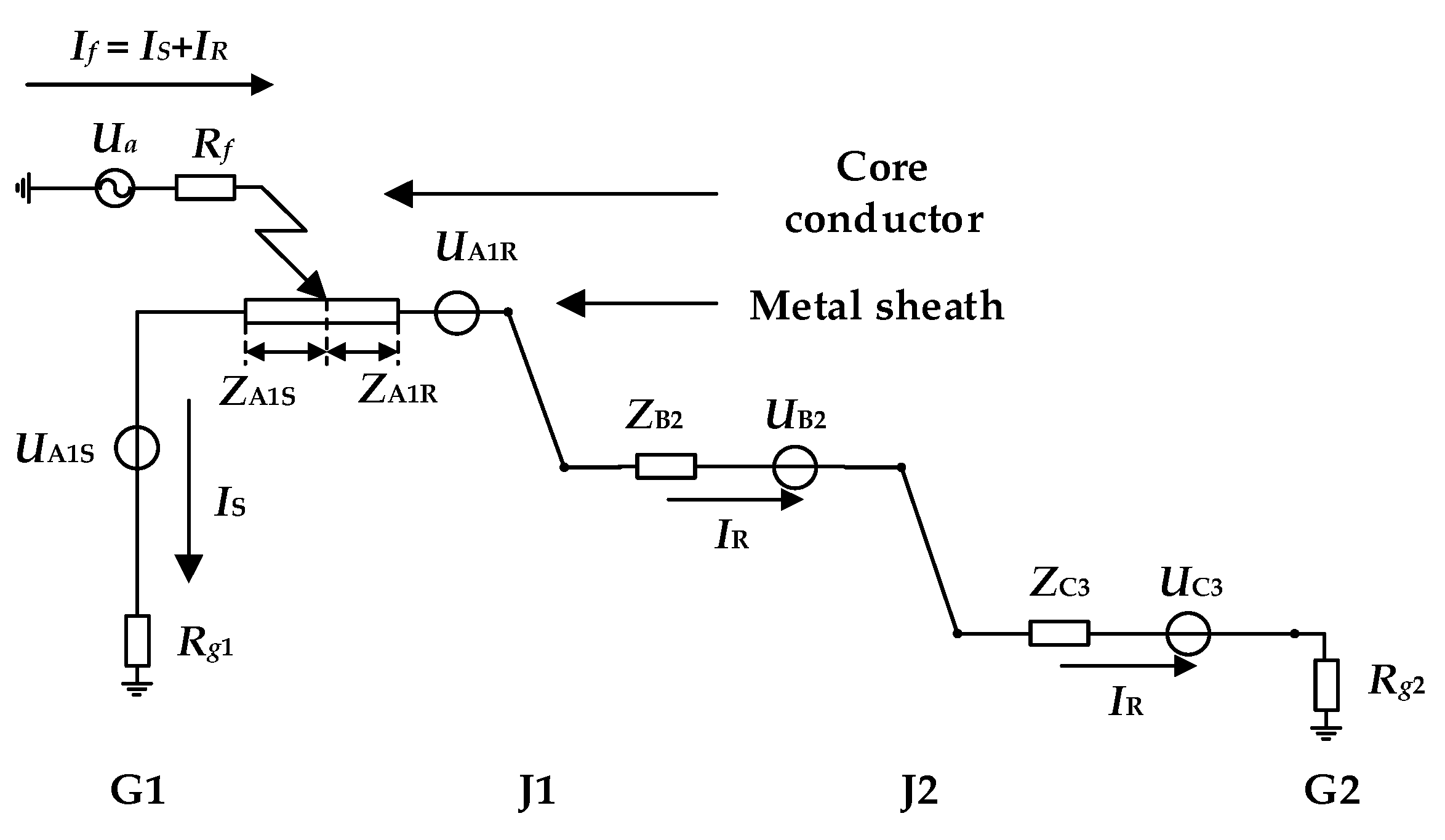
3. HV Cable Fault Location Model

3.1. HV Cable Fault Location Model

In [23], based on the calculation of the phase angle of the sheath circulation, a fault location criterion for high-voltage cross-connected cables is proposed. The model and cable structure parameters are used in this paper, as shown in Figure 1.

A typical HV cable consists of at least 5 layers, as shown in Figure 1. The core conductor carries the load current, and the metal sheath is grounded. Cables with a length of more than 1.2 km are mostly grounded by cross-bonded, as shown in Figure 2. The fault studied in this paper is mainly a short-circuit fault caused by the breakdown of the main insulation, and the fault location is mainly realized by analyzing the grounding current of the sheath, because the monitoring of the sheath current is relatively safer and easier to obtain.

In a major section, under normal operating conditions, the equivalent circuit model of the sheath current of the A1-B2-C3 section is shown in Figure 3. The calculation expression of the sheath current is shown in (7), where I_m1 represents the sheath current of the A1-B2-C3 section, U_a1 represents the induced electromotive force of the sheath section A1, and U_b2 represents the induced electromotive force of the sheath section B2, U_c3 is the induced electromotive force of the sheath section C3, Z_ma1 is the equivalent impedance of the sheath section A1, Z_mb2 is the equivalent impedance of the sheath section B2, Z_mc3 is the equivalent impedance of the sheath section C3, R_g1 Indicates the grounding resistance of the G1 end, and R_g2 indicates the grounding resistance of the G2 end. U_a1, U_b2, U_c3 contain the equivalent induced electromotive force of adjacent lines.

Since half of the leakage current flows in the same direction as the sheath circulating current and the other half is opposite to the sheath circulating current, it can be ignored in the calculation of the sheath grounding current under normal operation. When the short-circuit fault occurs, the equivalent circuit of the sheath current is changed, and the calculation method of the elements in the corresponding transmission line equation is also changed. During the short-circuit fault, the fault current flows from the core conductor into the metal sheath, and then flows to the ground through the metal sheath. A new current loop is formed between the core conductor and the metal sheath, and this current loop contains its own loop self-inductance and mutual inductance with other current loops. Taking the short-circuit fault in section A1 as an example, the equivalent circuit of the fault is shown in Figure 4, where U_a represents the equivalent voltage source of the A-phase line, U_A1S represents the induced electromotive force of the metal sheath section from G1 to the fault location, U_A1R represents the induced electromotive force of the metal sheath section from the fault location to J1, R_f represents the fault resistance, I_f represents the fault current of the power supply terminal, I_S represents the fault current flowing to G1 terminal, and I_R represents the fault current flowing to the G2 terminal.

The expressions of I_S and I_R are shown in (7) and (8), where Z_A1S represents the equivalent impedance of the metal sheath section from G1 to the fault position, and Z_A1R represents the equivalent impedance of the metal sheath section from the fault position to J1. For the specific solution method of each parameter, see reference [23], and the position of the fault point can be calculated by the phase difference P(section) between I_S and I_R. For example, P(A1) represents the phase difference between I_S and I_R of A1 section, the sheath currents are measured at G1 and J1.

$$I_S=\frac{U_a+U_{A1S}}{Z_{A1S}+R_f+R_{g1}}$$

(7)

$$I_R=\frac{U_a+U_{A1R}+U_{B2}+U_{C3}}{Z_{A1R}+Z_{B2}+Z_{C3}+R_f+R_{g2}}$$

(8)

3.2. Case Study of the Fault Location of HV Cable

In a simple power system consisting of a voltage source, a transformer, a complete cross-connected section of high-voltage cables, and three-phase balanced loads, the high-voltage cables were laid in three-phase tunnels in a zigzag pattern with a phase spacing of 0.3 m and a height of 0.5 m above the ground. The complete cross-connection section had a total length of 1500 m, each small section was 500 m long, and the grounding resistance of the direct grounding point of the metal sheath was 0.1 Ω. The soil resistivity was 100 Ωm. The cross-section of the core conductor was 800 mm², and the rated current carrying capacity was 976 A. The structural parameters are shown in

Table 1. Parameters of cross-sectional structure of the cable ¹.

Serial Number	Structure	Outer Radius/mm
1	Core conductor (copper)	17.0
2	Inner semi-conductive shield	18.4
3	Main insulation (cross-linked polyethylene, XLPE)	34.4
4	Outer semi-conductive shield	35.4
5	Water-blocking layer (semiconductor material)	39.4
6	Metal sheath (aluminum)	43.9
7	Jacket (Polyvinyl chloride, PVC)	48.6

(¹ The designation of the cable is YJLW03).

.

The three-phase voltage source of 110 kV was set to U_a = 63.51∠0° kV, U_b = 63.51∠−120° kV, U_c = 63.51∠120° kV, the three-phase balanced load ran at full load, and the short-circuit fault was set in the A1 section. According to the research on the breakdown characteristics of cross-linked polyethylene materials in [24], the conductivity of the penetrating main breakdown channel was about 10⁻³ Ω·cm. According to this calculation, the resistance of the breakdown channel of the main insulation of the cable was only a few milliohms, depending on the equivalent cross-sectional size of the breakdown channel. In addition, considering that there may have been a small contact resistance at the cross-bonded point, based on the above analysis, in this case, the transition resistance R_f was set to 0.01 Ω, and the fault point distance L_x was set as an independent variable. Since the length of the cable section A1 was 500 m, the variation range of L_x was (0, 500), so that the fault point can traverse any point in the section, the calculated phase difference P(A1) of the sheath current at both ends of the section A1 is shown in Figure 5.

4. Fault Location Simulation Analysis Based on UQ Method

4.1. The Simulation Based on the Three UQ Methods

At present, the accuracy of fault location is limited by the uncertainty factors of the actual fault scene. This paper mainly studies three common uncertainty factors: the resistivity of the sheath per unit length, the uneven distribution of the capacitance, and the length of the line section.

Three UQ methods such as MCS method, PCE method, and UDRM were respectively used to quantitatively analyze the uncertainty in HV cable fault location. Taking the parameters in the calculation example in Section 3.2 as the reference value, the change rate of the studied uncertainty factors was 50% random and uniform distribution, and the output changes of the sheath current and the fault location criterion were calculated and analyzed.

(1)

MCS method. The MCS method is generally used as a benchmark for methods in the field of uncertainty quantification. When using the MCS method to calculate the uncertainty of the resistivity per unit length of the HV cable fault location problem, it mainly includes the following steps: (a) according to the given distribution type, N samples are randomly generated; (b) substitute the N samples into the HV cable fault location calculation model in turn, and repeat the calculation to obtain the corresponding N sample output values; (c) calculate the relevant statistical characteristics of the sheath current, such as mean, standard deviation, probability density distribution, etc.

First, the relationship between the MCS mean convergence rate and N under normal operating conditions was calculated as shown in Figure 6a. When the number of samples reaches 300, the result tends to converge. Under the condition of short-circuit fault, the mean convergence rate of the fault location criterion was calculated respectively when the short-circuit point was 50–500 m, as shown in Figure 6b, when the number of samples reaches 300, the result tends to converge. Therefore, in the follow-up study, the sample size was chosen to be 500.

(2)

PCE method. The focus of the PCE method is the construction of a polynomial model, and then quantitative analysis is performed on its model. The fault location model of high-voltage cables is expressed as a polynomial model shown in (1), and N sampling points are selected in the standard random space and transformed into the original random space. Next, select an appropriate method to obtain the PCE coefficient, and calculate the probability and statistical characteristics of the sheath current value. Considering that the truncation order of the PCE method may have an influence on the calculation results, the PCE methods of the second-order expansion (p = 2), the third-order expansion (p = 3), and the fourth-order expansion (p = 4) were used for simulation.

(3)

UDRM. When using the UDRM method, the parameters in the calculation example in Section 3.2 are used as reference values, and the fault location model of the HV cable is expressed as the type shown in (2). Then, the number of integration nodes m corresponding to the random input variables of each dimension is determined. Calculate the corresponding 1-dimensional Gaussian nodes and weights according to the random input variable type, and substitute the given uncertainty factor range into the single-variable element calculation of (6). Thus, the statistical moment of the output voltage of the model can be calculated.

4.2. Quantitative Analysis of the Results

In order to quantitatively evaluate the uncertainty quantification results, parameters such as mean and standard deviation are usually used to describe the output uncertainty information. When there are a large number of samples, m is the arithmetic mean of the samples, as shown in (9).

$$\mu ={\displaystyle \underset{\mathrm{\Omega }}{\int }X{f}_X\left(X\right)}dX$$

(9)

The standard deviation s indicates the degree of deviation of the random variable distribution X from its mean. The smaller the standard deviation, the more concentrated the distribution of sample points.

$$\sigma =\sqrt{E{\left(X-\mu \right)}^2}=\sqrt{{\displaystyle \underset{\mathrm{\Omega }}{\int }{\left(X-\mu \right)}^2{f}_X\left(X\right)}dX}$$

(10)

Covariance (Cov) is used to describe the relationship between variables, as shown in (11), where $\overline{X}$ and $\overline{Y}$ are the mean values of variables X and Y, respectively.

$$Cov=\frac{{\displaystyle \sum _{i=1}^N\left(X_i-\overline{X}\right)\left(Y_i-\overline{Y}\right)}}{N-1}$$

(11)

The coefficient of variation (Cvar) measures the degree of dispersion of the predicted values of the model, also known as the “dispersion coefficient”, which represents the stability of the model. The expression of Cvar is shown in (12). Different Cvar values represent different stability situations, and the model stability quantification table is shown in

Table 2. Model stability quantization table.

Cvar	Model Stability
≤0.2	The fluctuation is very small and very stable
>0.2, ≤0.4	Small fluctuations, basically stable
>0.4, ≤0.6	Generally volatile, less stable
>0.6, ≤0.8	High volatility, unstable
>0.8	Highly variable and random

.

$$C\mathit{var}=\left|\frac{\sigma }{\mu }\right|$$

(12)

The mean absolute error (Mape) is used to discriminate the prediction accuracy of the model, and its expression is shown in (13), where N is the number of samples, u is the actual value, and û is the model predicted value.

$$Mape=\frac{1}{N}{\displaystyle \sum _{i=1}^N\frac{\left|u-\widehat{u}\right|}{u}}$$

(13)

The probability distribution of the sheath current I_m1 (under normal operation) and the fault location criterion P(A1) at a distance of 50 m from the head end of the short-circuit fault point were calculated respectively, under 50% amplitude variation range of three uncertainty factors, the resistivity of the sheath per unit length, the equivalent grounding resistance on both sides, and the length of the cable sections. The results of the statistical parameters are shown in

Table 3. Evaluation table of different UQ methods under 50% uncertainty of sheath resistivity under normal operation.

Methods	m	s	Cov	Cvar	Mape	t/s
MCS	0.1492	0.0025	0.0026	0.3386	0.2975	0.133
PCE_2	0.1393	0.0187	0.0004	0.1346	0.1023	0.554
PCE_3	0.1384	0.0180	0.0003	0.1304	0.1000	0.572
PCE_4	0.1373	0.0176	0.0003	0.1285	0.0990	0.651
UDRM	0.1498	0.0486	0.0024	0.3247	0.2891	0.438

,

Table 4. Evaluation table of different UQ methods under 50% uncertainty of the grounding resistance under normal operation.

Methods	m	s	Cov	Cvar	Mape	t/s
MCS	0.1363	5.39 × 10−6	2.91 × 10−11	3.96 × 10−5	3.46 × 10−5	0.183
PCE_2	0.1363	2.37 × 10−6	5.65 × 10−12	1.74 × 10−5	0	0.547
PCE_3	0.1363	2.30 × 10−6	5.31 × 10−12	1.69 × 10−5	0	0.629
PCE_4	0.1363	2.32 × 10−6	5.37 × 10−12	1.70 × 10−5	0	0.685
UDRM	0.1362	2.08 × 10−7	4.33 × 10−14	1.53 × 10−6	0.0004	0.429

,

Table 5. Evaluation table of different UQ methods under 50% uncertainty of the cable length under normal operation.

Methods	m	s	Cov	Cvar	Mape	t/s
MCS	0.1488	0.0478	0.0023	0.3212	0.2819	0.121
PCE_2	0.1389	0.0178	3.16 × 10−4	0.1281	0.1009	0.541
PCE_3	0.1395	0.0192	3.70 × 10−4	0.1379	0.1110	0.553
PCE_4	0.1385	0.0178	3.18 × 10−4	0.1287	0.0991	0.688
UDRM	0.1306	0.0032	1.04 × 10−5	0.0248	0.0417	0.408

,

Table 6. Evaluation table of different UQ methods under 50% uncertainty of sheath resistivity under short-circuit fault.

Methods	m	s	Cov	Cvar	Mape	t/s
MCS	177.95	0.1639	0.0269	9.21 × 10−4	7.79 × 10−4	12.78
PCE_2	178.07	0.0674	0.0045	3.79 × 10−4	1.07 × 10−4	13.12
PCE_3	178.08	0.0655	0.0043	3.68 × 10−4	1.22 × 10−4	13.14
PCE_4	178.16	0.0646	0.0042	3.62 × 10−4	3.98 × 10−4	13.45
UDRM	178.12	0.0102	1.04 × 10−4	5.72 × 10−5	1.94 × 10−4	13.33

,

Table 7. Evaluation table of different UQ methods under 50% uncertainty of sheath resistivity under short-circuit fault.

Methods	m	s	Cov	Cvar	Mape	t/s
MCS	177.96	0.3282	0.1077	0.0018	7.06 × 10−4	12.89
PCE_2	178.07	0.1317	0.0174	7.40 × 10−4	1.13 × 10−4	13.27
PCE_3	178.07	0.1301	0.0169	7.31 × 10−4	8.08 × 10−5	13.28
PCE_4	178.06	0.1314	0.0173	7.38 × 10−4	1.70 × 10−4	13.42
UDRM	178.13	0.0253	6.40 × 10−4	1.42 × 10−4	2.51 × 10−4	13.32

and

Table 8. Evaluation table of different UQ methods under 50% uncertainty of the cable length under short-circuit fault.

Methods	m	s	Cov	Cvar	Mape	t/s
MCS	177.96	0.0139	1.94 × 10−4	7.84 × 10−5	7.10 × 10−4	12.93
PCE_2	178.05	0.0055	3.06 × 10−4	3.11 × 10−5	2.34 × 10−4	13.53
PCE_3	178.12	0.0060	3.58 × 10−5	3.36 × 10−5	1.95 × 10−4	13.49
PCE_4	178.09	0.0056	3.11 × 10−5	3.13 × 10−5	1.90 × 10−5	13.43
UDRM	178.09	0.0011	1.22 × 10−6	6.19 × 10−6	3.30 × 10−5	13.37

and the probability density distribution plot of the results are shown in Figure 7, Figure 8, Figure 9, Figure 10, Figure 11 and Figure 12.

It is to be noted that all the calculations presented in the paper were performed using MATLAB, and the simulations were carried out on an AMD Ryzen Threadripper 3970X 32-Core, 64 GB RAM computer. As presented in Table 3, Table 4, Table 5, Table 6, Table 7 and Table 8 and Figure 7, Figure 8, Figure 9, Figure 10, Figure 11 and Figure 12, the five UQ methods have good effects on the quantification of the uncertain factors when the sample size is sufficient. The mean values of the results of these five methods are relatively close, but the distributions are quite different. In general, the distribution of results of UDRM is relatively concentrated, while the distribution of results of MCS is relatively scattered. Specifically, under 50% amplitude variation range of three uncertainty factors, the changes in sheath resistivity make the waveform flatter, while the changes in cable length make the waveform more spread out by different methods, whether in normal operation or short-circuit fault conditions. Under 50% amplitude variation range of grounding resistance, all the distributions of results of these five methods are relatively concentrated. The probability density of the calculated data of P(A1) using the five different methods under 50% uncertainty of the cable length under short-circuit fault condition is the most scattered. For the condition of normal operation or short-circuit fault condition, the waveforms in normal operation are flatter.

5. Discussion

In order to study the feasibility and effectiveness of the UQ method in the problem of HV cable fault location, MCS, PCE, and UDRM were studied and compared with each other. It can be seen from the simulation results of the HV cable that when the MCS method is used for the quantitative analysis of uncertainty, the sample mean convergence rate is relatively low, and only when the number of N is large enough, a smooth probability distribution curve can be obtained, which costs a lot of time. Especially for the fault location in practice, it is almost impossible to withstand hundreds of tests to calculate the fault position. The PCE method has higher accuracy, and with the increase of the polynomial order p, the uncertainty calculation results are more accurate. However, the running time of PCE is relatively long, and with the increase of uncertain factors, greater nonlinearity may lead to an exponential increase in the computational scale of PCE, which in turn makes it impossible to solve. The quantification results using UDRM are very close to the results of the MCS and PCE, while the mean convergence rate is significantly higher, and the distribution of the results is more concentrated, which is a great advantage for practical applications.

However, the actual experiments and applications on the HV cables are still premature. For example, the settings and verification problems of the uncertain factors in practice, and the maximum number of tests and cost issues that can be accepted. These will be further studied in the future.

6. Conclusions

The paper conducted a prospective study on the application of three UQ methods, MCS, PCE, and UDRM, in HV cable fault location. The sheath resistivity per unit length, the equivalent grounding resistance on both sides, and the length of the cable section were taken as the uncertainty factors. The simulation results indicate that:

(1)

The UQ methods are effective for the simulation analysis of the fault location, and UDRM has certain application prospects for HV fault location in practice.

(2)

The quantification results of MCS, PCE, and UDRM are very close, while the mean convergence rate is significantly higher for UDRM.

(3)

Compared with MCS, PCE, and UDRM, PCE and UDRM have higher accuracy, MCS and UDRM require less running time.

References

1. Zhou, C.; Yi, H.; Dong, X. Review of recent research towards power cable life cycle management. High Volt. 2017, 2, 179–187. [Google Scholar] [CrossRef]
2. Teng, C.; Zhou, Y.; Wu, C.; Zhang, L.; Zhang, Y.; Zhou, W. Optimization of the Temperature-Dependent Electrical Resistivity in Epoxy/Positive Temperature Coefficient Ceramic Nanocomposites. IEEE Trans. Dielectr. Electr. Insul. 2021, 28, 468–475. [Google Scholar] [CrossRef]
3. Montanari, G.C.; Hebner, R.; Morshuis, P.; Seri, P. An approach to insulation condition monitoring and life assessment in emerging electrical environments. IEEE Trans. Power Deliv. 2019, 34, 1357–1364. [Google Scholar] [CrossRef]
4. Suonan, J.; Qi, J. An accurate fault location algorithm for transmission lines based on R-L model parameter identification. Electr. Power Syst. Res. 2005, 76, 17–24. [Google Scholar] [CrossRef]
5. Eissa, M. Ground distance relay compensation based on fault resistance calculation. IEEE Trans. Power Deliv. 2006, 29, 1830–1835. [Google Scholar] [CrossRef]
6. Sheta, A.N.; Abdulsalam, G.M.; Eladl, A.A. Online tracking of fault location in distribution systems based on PMUs data and iterative support detection. Int. J. Electr. Power Energy Syst. 2021, 128, 106793. [Google Scholar] [CrossRef]
7. Xie, L.; Luo, L.; Li, Y.; Zhang, Y.; Cao, Y. A Traveling Wave-Based Fault Location Method Employing VMD-TEO for Distribution Network. IEEE Trans. Dielectr. Electr. Insul. 2020, 35, 1987–1998. [Google Scholar] [CrossRef]
8. Zhang, J.; Gong, Q.; Zhang, H.; Wang, Y.; Wang, Y. A Novel Pix2Pix Enabled Traveling Wave-Based Fault Location Method. Sensors 2021, 21, 1633. [Google Scholar] [CrossRef]
9. Yu, K.; Zeng, J.; Zeng, X.; Liu, F.; Zu, Y.; Yu, Q.; Zhuo, C. A novel traveling wave fault location method for transmission network based on time linear dependence. Int. J. Electr. Power Energy Syst. 2021, 126, 106608. [Google Scholar] [CrossRef]
10. Dashti, R.; Salehizadeh, S.M.; Shaker, H.R.; Tahavori, M. Fault Location in Double Circuit Medium Power Distribution Networks Using an Impedance-Based Method. Appl. Sci. 2018, 8, 1034. [Google Scholar] [CrossRef]
11. Bahmanyar, A.; Jamali, S. Fault location in active distribution networks using non-synchronized measurements. Int. J. Electr. Power Energy Syst. 2017, 93, 451–458. [Google Scholar] [CrossRef]
12. Dashti, R.; Ghasemi, M.; Daisy, M. Fault location in power distribution network with presence of distributed generation resources using impedance based method and applying π line model. Energy 2018, 159, 344–360. [Google Scholar] [CrossRef]
13. Lopes, F.V.; Dantas, K.M.; Silva, K.M.; Costa, F.B. Accurate Two-Terminal Transmission Line Fault Location Using Traveling Waves. IEEE Trans. Power Deliv. 2018, 33, 873–880. [Google Scholar] [CrossRef]
14. Borghetti, A.; Bosetti, M.; Nucci, C.A.; Paolone, M. Integrated Use of Time-Frequency Wavelet Decompositions for Fault Location in Distribution Networks: Theory and Experimental Validation. IEEE Trans. Power Deliv. 2010, 25, 3139–3146. [Google Scholar] [CrossRef]
15. Alexandre, P.; Alves, S.; Antonio, C.S.L.; Suzana, M.S. Fault location on transmission lines using complex-domain neural networks. Electr. Power Energy Syst. 2012, 43, 720–727. [Google Scholar]
16. Preece, R.; Milanovic, J.V. Assessing the Applicability of Uncertainty Importance Measures for Power System Studies. IEEE Trans. Power Syst. 2016, 31, 2076–2084. [Google Scholar] [CrossRef]
17. Feinberg, J.; Langtangen, H.P. Chaospy: An Open Source Tool for Designing Methods of Uncertainty Quantification. J. Comput. Sci. 2015, 11, 46–57. [Google Scholar] [CrossRef] [Green Version]
18. Yasuda, M.; Sekimoto, K. Spatial Monte Carlo integration with annealed importance sampling. Phys. Rev. E 2021, 103, 052118. [Google Scholar] [CrossRef]
19. Fox, J.; Kten, G. Polynomial Chaos as a Control Variate Method. SIAM J. Sci. Comput. 2021, 43, A2268–A2294. [Google Scholar] [CrossRef]
20. Yuan, X.; Liu, S.; Valdebenito, M.A.; Faes, M.G.R.; Jerez, D.J.; Jensen, H.A.; Beer, M. Decoupled reliability-based optimization using Markov chain Monte Carlo in augmented space. Adv. Eng. Softw. 2021, 157–158, 103020. [Google Scholar] [CrossRef]
21. Bhusal, R.; Subbarao, K. Generalized Polynomial Chaos Expansion Approach for Uncertainty Quantification in Small Satellite Orbital Debris Problems. J. Astronaut. Sci. 2020, 67, 225–253. [Google Scholar] [CrossRef]
22. Tripathy, R.K.; Ilias, B. Deep UQ: Learning deep neural network surrogate models for high dimensional uncertainty quantification. J. Comput. Phys. 2018, 375, 565–588. [Google Scholar] [CrossRef] [Green Version]
23. Li, M.; Zhou, C.; Zhou, W. A Revised Model for Calculating HV Cable Sheath Current under Short-circuit Fault Condition and Its Application for Fault Location—Part 1: The Revised Model. IEEE Trans. Power Deliv. 2019, 34, 1674–1683. [Google Scholar] [CrossRef] [Green Version]
24. Vaughan, A.S.; Hosier, I.L.; Dodd, S.J.; Sutton, S.J. On the structure and chemistry of electrical trees in polyethylene. J. Phys. D-Appl. Phys. 2006, 39, 962–978. [Google Scholar] [CrossRef]
Figure 1. The schematic diagram of the structure and sheath current of HV cable. In the equivalent circuit, Zc represents the equivalent impedance of the core conductor, Ri represents the equivalent resistance of the main insulation, Ci represents the equivalent capacitor of the main insulation, ZmL represents the equivalent impedance of the left half of the metal sheath, ZmR represents the equivalent impedance of the right half of the metal sheath, ZmLk represents the equivalent ground impedance of the metal sheath on the left side, ZmRk represents the equivalent ground impedance of the metal sheath on the right side.
Energies 15 08447 g001
Figure 2. The schematic diagram of a cross-bonded HV cable.
Energies 15 08447 g002
Figure 3. The equivalent circuit of sheath current in A1–B2–C3 section under normal operation.
Energies 15 08447 g003
Figure 4. The equivalent circuit of sheath current when a short circuit fault occurs in section A1.
Energies 15 08447 g004
Figure 5. The phase difference between fault current IS and fault current IR when the fault occurred in cable section A1.
Energies 15 08447 g005
Figure 6. Mean convergence rate of MCS. (a) Normal operation. (b) Short-circuit fault.
Energies 15 08447 g006
Figure 7. The probability density of the calculated data of Im1 using the 5 different methods under 50% uncertainty of sheath resistivity under normal operation.
Energies 15 08447 g007
Figure 8. The probability density of the calculated data of Im1 using the 5 different methods under 50% uncertainty of grounding resistance under normal operation.
Energies 15 08447 g008
Figure 9. The probability density of the calculated data of Im1 using the 5 different methods under 50% uncertainty of the cable length under normal operation.
Energies 15 08447 g009
Figure 10. The probability density of the calculated data of P (A1) using the 5 different methods under 50% uncertainty of sheath resistivity under short-circuit fault condition.
Energies 15 08447 g010
Figure 11. The probability density of the calculated data of P (A1) using the 5 different methods under 50% uncertainty of grounding resistance under short-circuit fault condition.
Energies 15 08447 g011
Figure 12. The probability density of the calculated data of P (A1) using the 5 different methods under 50% uncertainty of the cable length under short-circuit fault condition.
Energies 15 08447 g012