Decomposition of a Cooling Plant for Energy Efficiency Optimization Using OptTopo

Abstract

The operation of industrial supply technology is a broad field for optimization. Industrial cooling plants are often (a) composed of several components, (b) linked using network technology, (c) physically interconnected, and (d) complex regarding the effect of set-points and operating points in every entity. This leads to the possibility of overall optimization. An example containing a cooling tower, water circulations, and chillers entails a non-linear optimization problem with five dimensions. The decomposition of such a system allows the modeling of separate subsystems which can be structured according to the physical topology. An established method for energy performance indicators (EnPI) helps to formulate an optimization problem in a coherent way. The novel optimization algorithm OptTopo strives for efficient set-points by traversing a graph representation of the overall system. The advantages are (a) the ability to combine models of several types (e.g., neural networks and polynomials) and (b) an constant runtime independent from the number of operation points requested because new optimization needs just to be performed in case of plant model changes. An experimental implementation of the algorithm is validated using a simscape simulation. For a batch of five requests, OptTopo needs 61$\min$ while the solvers Cobyla, SDPEN, and COUENNE need 0.3 min, 1.4 min, and 3.1 min, respectively. OptTopo achieves an efficiency improvement similar to that of established solvers. This paper demonstrates the general feasibility of the concept and fortifies further improvements to reduce computing time.

1. Introduction

Using energy as efficiently as possible is a key challenge of our time. For the manufacturing sector, this motivates investment in more efficient machinery as well as approaches to use existing facilities more efficiently. This paper contributes to the latter, specifically to the set-point optimization of complex systems by means of decomposition. As an example of a complex system serves a refrigerating plant consisting of a cooling tower, a cooling water cycle, two chillers, and a chilled water cycle. A simulation in Simscape^TM using MATLAB/Simulink is available under [1].

The here proposed method OptTopo (Optimization based on topology) uses the physical topology information about the plant structure to model components separately and organize these potentially heterogeneous models in a graph. We apply an established method for energy performance indicators (EnPI) designed by ÖKOTEC Energiemanagement GmbH to formulate an optimization problem [2]. According to the EnPI-methodology [3], relevant parameters are classified as either efforts, set-points, external parameters or benefits. Figure 1 illustrates the general structure of the system with these parameters assigned. The green boxes highlight the variables which can be used for the optimization: pressure values for the water circulations, set temperature for the cooling tower, and the switch-off temperature for two chillers. Thus, five variables can be used.

The research goal of this paper is to demonstrate that the optimization problem can be solved recursively by the optimization algorithm OptTopo which traverses the graph containing all component models. A draft of the approach was first presented in 2020 [4]. Further details about performance measures are given in [5].

This paper is structured as follows. Section 2 presents seven approaches for similar problems to illustrate the context of this work. The concept of OptTopo is introduced in Section 3, while implementation, experiments, and results follow in Section 4. Section 5 gives a conclusion and a brief outlook.

2. Related Work

This section summarizes some approaches for calculating optimal set-points for coupled systems without any claim to expound a systematical review. The projects described aim to optimize more or less complex systems by means of supervisory control. According to Behrooz et al. [6], the term supervisory control refers to algorithms “pursuing the minimization or maximization of a real function by systematically selecting values of parameters or variables within acceptable ranges”. Correspondingly, we address techniques that steer physically inter-connected systems to increase their overall energy efficiency. We mainly consider the field of heating ventilation air conditioning (HVAC), except from two approaches (Section 2.4 and Section 2.5) with the demonstration of how the operation of machine tools uses graph theory and reinforcement learning, respectively. These methods are also of interest for the optimization of cooling plants and, thus, are discussed here as well.

2.1. Cascade Control for Coupled HVAC Systems

Komareji et al. considers a system that consists of several heat exchangers whose set temperatures are regulated by presetting the volume flows of air and water [7]. A primary, a secondary, and a tertiary circuit are coupled, the first transition being realized by an air-air heat exchanger, the second by an air-water heat exchanger. For clarity, the relationships are modeled as static polynomials. Since polynomial functions up to the third degree are used, it is a nonlinear problem that is potentially nonconvex. The numerical calculation is not detailed in the article, but the decomposition of interconnected utilities and the modeling with static functions is described as an example. With Komareji [7,8], the optimization is performed using an objective function composed from the models per component. Thus, the optimization works for coupled systems but not along the topology because all manipulated variables are changed in the overall model. A non-convex model with only continuous variables is explicitly assumed. Combining all terms of energy consumption to a common objective function is a very common approach but leads to an optimization problem with all variables of the entire system. OptTopo, in contrast, aims to find optimal set-points for each subsystems separately.

2.2. Multiplexed Real-Time Optimization

Asad et al. presented Multiplexed Real-Time Optimization (MRtOpt) applied to an air-conditioning system of an office building [9,10]. Their approach realizes a supervisory cascade for several locally controlled units to reduce total energy consumption. The authors vividly present the mutual influence of the involved subsystems, which emphasizes the complexity of the resulting optimization problem. An interior point method is used to solve the posed optimization problem.

The testing was carried out using a simulation with the established tool TRNSYS. The authors point out potentially undesirable deviations in the presence of abrupt changes in set-points [10] and design separate models for predicting these effects, both for the actuated control loop and for neighboring entities physically affected by the change. The models are determined by sub-space system identification. An adaptive variant of the method was published in 2019 [11]. The MRtOpt, according to Asad et al., is applied to a system of several components, thus, optimizing coupled systems, but as a joint objective function without considering the topology. Polynomials are used, making the models transferable and transparent. A convex and continuous problem is assumed.

2.3. Extremum Seeking Control (ESC)

In a collaboration between Whirlpool Cooperation, Johnson Controls Inc., and the University of Texas, Baojie et al. investigated the optimization of a refrigeration system consisting of two chillers operating parallel, a cooling tower, and associated water circuits [12]. The authors first distinguish between rule-based, model-based, and model-free optimization. ESC is used, where the gradient is estimated online. The system is stimulated by a peripheral signal (in this case, a sinusoidal oscillation). Due to the provoked variation around the operating point, the gradient can be estimated robustly. This is integrated into the control so that the operating point is shifted in real-time in the direction of lower energy consumption.

Addressed manipulated variables are the speed values of the chilled water pumps, the ventilation of the cooling tower, and the supply temperatures of the chillers. The authors assume the input and output dynamics each as a linear time-invariant system, thus, encapsulating any nonlinearities as a static model and assuming the convexity of the optimization problem. The control itself is performed by a PI controller. When the manipulated variable is constrained, the integrator may ineffectively assume an unrealistically high value without reaching the distance accordingly. This wind-up effect poses the risk that the integrator value cannot be decayed fast enough when the motion is in the opposite direction. As a remedy, Ying et al. [13] presented an anti-windup solution for ESC controls.

Complementing the presented method, Salsbury et al. published an automatic selection of the considered input variables [14]. The starting point is a dither signal composed of several oscillations to stimulate the system dynamics. Here, for inputs, it is checked concurrently whether there is either no coupling or a weak or strong coupling. This is done by means of singular value decomposition. Thus, only those couplings with large singular values are considered to keep the complexity of the optimization problem low. This ESC approach was tested on a Modelica simulation [12] with anti-windup control and in [14] with automatic input selection.

Analogous to Komareji [7,8], the ESC designed by Salsburg forms a objective function containing separate terms for each component. In contrast to Komareji, however, no prefabricated models are used. Empirical estimation of the gradient allows the model-free descent on the objective function, which is assumed to be convex and continuous for this purpose.

2.4. Optimization of Machine Tools Using Graph Models

Working in the ECOMATION research group dedicated to efficient machine tool operation, Eberspächer and Schlechtendahl [15,16] describe a graph of states that is also developed from a consideration of the components, leading to the optimization of coupled systems. The optimization is a set of rules to navigate along this state machine. Any continuous and integer values can be stored in the nodes of this state machine, but the optimization is still the selection of solutions from a finite set. This means that there is no need to distinguish between integer and real values here, and in particular, convexity is not a category in this context. This approach is related to OptTopo but does not necessarily consider Kirchhoff’s law for nodes with respect to energy flows because machine tools do not have the chained energy transformation like cooling plants do.

2.5. Multi-Agent Reinforcement Learning (MARL) in Machine Control

This approach was presented by Bakakeu in cooperation with the SIEMENS Digital Factory division [17,18]. With this algorithm, several machines are to run in such a coordinated manner that cumulated energy expenses, taking into account effects like self-generation and volatile energy prices, reaches an always up-to-date optimum. Reinforcement learning (RL) is based on the so-called Markov Decision Process, which assumes that changes in the defined state of the system only depend on the current state and considered actions. In the work of Bakakeu, this cannot be assumed for several machines with plenty of parameters each. Instead, machines are modeled separately. Thus, the Markov condition can no longer be assumed for the resulting ensemble because of mutual influence. Bakakeu proposes “a multi-agent actor-critic method that takes into account the policies of other participants to achieve explicit coordination between a large number of actors” [17].

The learning of the agents follows the scheme of the autocurricula [19], so that challenges are solved in both ways cooperatively and competitively. The agents learn the behavior of the surrounding machines along with the strategies of the agents behind them. The implementation uses Proximal Policy Optimization (PPO). The authors describe how the machines shut themselves down when overload threatens but act swiftly on changes in the situation and compete for supply phases that become available. Bakakeu’s MARL takes into account several components of a system, each with autonomous agents, which, however, partly collaboratively pursue common goals. The models are created by learning, so they are not directly transferable and also are not transparent. MARL can provide individual agents with different initial values, but this is not explicitly discussed in the paper. Integer values and binary states can easily be included in the state spaces of MARL.

2.6. Deep Reinforcement Learning

In 2019, Panten presented a study on the use of Deep Reinforcement Learning (DRL) to increase energy efficiency in supply technology [20]. Panten argues the necessity of machine learning methods with the increase in complexity of optimization tasks due to both the interconnection of many subsystems and the consideration of dynamic memory effects. For the latter, prediction functions are provided. The scalability of the optimization facilitates a hierarchical concept, which solves subproblems locally on a lower level, whereby only a fraction of the variables are considered in a higher-level optimization problem.

Panten builds a simulation of a complex system that includes a cooling tower, chillers, pumps, condensing boilers, immersion heaters, solar panels, and other elements, relying on the simulation standard functional mock-up interface (FMI) to organize the models created in Modelica. The components are each controlled locally, such as by hysteresis or PI controllers. The higher-level system behavior is learned by a deep neural network (DNN) using PPO as well. Reinforcement learning now optimizes continuous parameters on this system knowledge, which are passed to the lower-level control. The communication between the entities works via OPC UA. The entire approach is validated on simulation data using a functional model implemented in Python [21].

Panten’s approach is similar to the MARL of Bakakeu. Here, too, coupled systems are considered, but in Panten’s case the superimposed optimization takes place without local agents being pronounced for each entity. Thus, one cannot speak of optimization along the topology here. With the DNN approach, models cannot be interpreted manually nor transferred in a modular way. In this study, the optimization parameters are expressed as real numbers. In general, a generalization to integer and binary attributes should be possible here as well.

2.7. Optimization of Parallel Pumps

Wang and Zhao present a special case of using topology where six differently sized pumps interact to serve the flow and pressure demands with as little energy as possible [22,23]. These operating requirements are assumed to be quasi-static. The pumps can be turned on and off and their flow rate can be controlled via the rotational speed. The resulting energy consumption and volume flow are predicted on the basis of polynomials estimated from measured data.

The pumps operating in parallel each have controllers, which are connected to a network. This results in a network of agents that can be represented as a connected graph. A starting node sends messages to neighboring nodes, which identify themselves as child nodes, and also sends out messages until all (six in the example) nodes are marked. The nodes evaluate randomly chosen operating points along a uniform distribution. These include normalized speed $\omega$, flow Q, and electrical power P. The algorithm includes synchronous updates of this aggregation and replaces the value initialized by $P^{★}=\infty$ for the total power expended. For a sufficient number of iterations, this algorithm finds the optimal allocation of flow among the six pumps. For the example, the desired setting could be found with 20 iterations in under 3 $\mathrm{s}$. In the experiment, Zhao et al. apparently used the polynomials of the pump characteristics both for the solution algorithm and for validation, which makes it difficult to track. A more advanced publication by the same authors converts the method to asynchronous communication while preserving the basic principle [23].

This approach deals with coupled pumps but considers the topology only to establish a computational order and is limited to a parallel arrangement. Polynomials are deposited, which is why the models are interchangeable and transparent. The consideration of discrete states is conceivable but is not explicitly discussed.

2.8. Summary of Literature

Closely related to the given subject, Komareji [7], Asad [11] and Baojie [12] set up an overall cost function and varied the parameters of the resulting optimization problem accordingly. To our knowledge, there are no publications on approaches that use plant topology to decompose the overall system and optimize every subsystem following energy flows.

3. Concept

3.1. General Workflow to Optimize a System Based on Topology

Assume a cooling system consisting of chillers, pumps, and cooling towers as sketched in Section 1. Firstly, we assume that all these components are physically interconnected and considered separately from any (physically) independent systems. Given this system of coupled components, we propose an optimization method that works as a supervisory cascade. To implement this set-point optimization, we address the three following steps:

• For each component, assign the absorbed energy flow (e.g., electrical energy), generated output flow (called benefit), control variables, and external influence factors.
• Generate models to predict the in- and outgoing flows of all the subsystems. Since they are separated, these models can be of different forms for different subsystems, like polynomials for one and a neural network for another subsystem.
• Use the system decomposition (step 1) together with the models of the subsystems (step 2) and an objective function as input for an optimization algorithm using this topology.

As for step (2), it is important to see the advantage of being able to use different model types for the identified heterogeneous subsystems. In that way, problem-specific models (and, in consequence also, optimization procedures) can be used. In this research, the topology information connects these independent models as a more general interface for reunification and, thus, allows us to find the optimal set-point for the overall system instead of just combining the local optima of the subsystems. However, we do restrict the model types to be quasi-static [2]. In the work on hand, we model the flow through an individual subsystem as a static energy model, which we formalize via

$$f\left(\overrightarrow{\phi },\overrightarrow{\vartheta },\overrightarrow{\xi }\right)=\left(\overrightarrow{\alpha },\overrightarrow{\nu },\overrightarrow{\chi }\right).$$

(1)

Here, f is a static, potentially non-smooth function. We use energy performance indicators (EnPI) to describe every subsystem formally. The variable $\alpha$ denotes the effort, in our example energy input, $\nu$ denotes the benefit, for our system, the utilized energy output. The variable $\overrightarrow{\alpha }$ can be read as a vector consisting of multiple forms of energy being absorbed, e.g., electrical energy and natural gas. In this paper, we use the scalar form. The variable $\phi$ denotes a free parameter, which controls the adjustable set-points of the subsystem. On the left side of Equation (1), besides the free parameter, an external parameter $\vartheta$ considered in the constraints. To constrain thermal interconnections, we add an arbitrary but fixed parameter $\xi$ denoting properties in which subsystems have to match but for which there are no further requirements for their concrete values, e.g., a common temperature in a thermal equilibrium. On the right side, we are mainly interested in the resulting effort $\alpha$ and benefit $\nu$, but we can also define the internal variable $\chi$ to be observed. The energy efficiency is denoted $ϵ=\frac{\nu }{\alpha }$. For any system A, the set ${\mathrm{\Phi }}_A$ contains all free parameters $\phi$, and analogously ${\mathrm{\Xi }}_A$ is a set of $\xi$.

As described in step (1), to use topology information for the optimization of an interconnected system of subsystems, this topology information has to be encoded in a machine-readable way. We used a directed acyclic graph (DAG). That means that every subsystem is represented by models in the form of equation (1) and a node in a graph. As a result, the topology graph holds one node per component (e.g., cooling tower, chiller) and one edge for each energy flow (e.g., thermal conduction from cooling water to the chiller).

The connections of the models according to their topology need to reflect on conservation laws: If the benefit ${\nu }_A$ of subsystem A delivers the effort ${\alpha }_B$ for subsystem B, then their values have to be (approximately) equal. Evidently, the heat absorbed by a heat-exchanger needs to be released. These issues of defining appropriate performance indicators for industrial systems were further discussed in [2,4,5].

3.2. Optimization Algorithm Based on Topology

OptTopo is an attempt to decompose the subsystems to achieve problems with fewer dimensions. The idea of solving a complex problem by means of decomposition in smaller subproblems comes from the algorithmic paradigms Divide and Conquer and Dynamic Programming. We draw inspiration especially from the core idea of Dynamic Programming, known as Bellman’s principle, that the optimal solution for the overall system must also be optimal for the tail problems at any point in our procedure. In our case, the “tail“ from any point on is given by the direction of the flow through the directed graph.

Despite various forms of energy available (e.g., natural gas and electricity), we assume a virtual common source which is achieved by assigning prices to all energy sources considered. This leads to a unique root node serving as a starting point for OptTopo. So, we avoid a multi-objective optimization problem.

Furthermore, we assume a non-cyclic system and graph so that all edges (energy flows) direct themselves towards a common sink, e.g., the cooling power demanded by a manufacturing process. The optimization problem is now defined as follows: find, if possible, a configuration of the free variables of all the subsystems such that the request (at the sink) is satisfied with minimal energy demand (at the common root).

3.3. Boundedness and Discretization

In its present state, OptTopo uses a brute force search to optimize the elementary models for each subsystem, meaning that, at each subsystem, it computes Equation (1) for every possible combination of relevant parameters and saves only the best ones for each possible request (a certain benefit $\nu$ under constraints regarding $\vartheta$ and $\xi$). Hence, we assume the components of all parameter vectors to be contained in bounded intervals which can be discretized. These limitations concerning the parameters of the model could be avoided by applying other solvers (instead of brute force) to find optimal set-points for every subsystem. In the current state, we presume boundedness and proper discretization.

3.4. Topological Sorting and Graph Traversal for Optimization

The topology information is encoded in the graph structure of the problem with energy flows as edges between individual subsystems (nodes). OptTopo uses this information to solve the overall optimization problem by optimizing it from left to right—which we take to be the imaginary direction of the energy flows. This means that OptTopo creates a topological sorting of the nodes of the graph. The problem of topological sorting was discussed in 1962 by Kahn [24]. The topological ordering simply follows the paths of the energy flows and if two components are both children of a common parent node (with no edge between them pointing to one or the other), they are randomly ordered.

Given this sorting, every subsystem can be optimized using brute force regarding the primary effort caused in the root node—because every predecessor node is already optimized and, thus, holds the most efficient set-points and the anticipated quantities for effort and benefit. In other words: once all predecessors of a component have been optimized, the different efficiencies for all the energy conversions in the path are known, respectively. This information can be propagated along the path through all predecessors to the current node. This strict procedure gives commensurable efforts in every component to be optimized and allows one to calculate the efficiency in a certain node with reference to a common source (e.g., primary energy or cost).

Topological sorting gives an unambiguous sequence of nodes. Therefore, every node has a set of preceding nodes. We call this set of nodes, including the respective edges, the ancestor system. At every point of the graph traversal, OptTopo can access the already calculated optimal values $(\alpha ,\nu )$ valid for the current request. This ensures that every node in the graph can be optimized on the basis of the solutions for every ancestor node.

As pointed out before, this sequential brute-force computation from left to right by graph traversal would not be possible without discretization (i.e., with infinite sets of possible values for the benefits) since the storage capability is, of course, limited. However, with further developments of OptTopo, especially the data structures and procedures that are better optimized, the granularity of the discretization can be designed to be sufficient.

3.5. Solution Look-Up

When the graph traversal is complete, meaning that OptTopo has optimized all the components, the optimal configuration for any request in the given discretization can be received by a simple look-up. This is a great advantage compared to conventional optimizers, which would have to solve an individual problem for every demanded request. OptTopo, however, can solve multiple requests with no additional computation required.

For a certain request at the sink (e.g., 100 $\mathrm{k}$$\mathrm{W}$ of cooling power), the sink node has stored its own optimal settings and its demands regarding its direct predecessors. Metaphorically speaking: the chilled water cycle requests for a certain level of cooling from the chiller, which knows its most efficient operation points and infers its demand for cooling supplied by the cooling water cycle, which is fed by the cooling tower. Obviously, new requests do not evoke any recalculation, but only a new propagation of the already known results.

4. Implementation and Experiments

For testing OptTopo, a test bed was designed as described in [4,5]. The main elements are

• a simulation of a cooling plant mentioned in Section 1 which provides data for model training—and allows to validate the resulting set-points,
• a python project for running different optimization routines on predefined problems,
• interfaces to dedicated solver libraries like Pyomo [25] and pyOpt [26].

This setup allows one to run OptTopo and other algorithms, which get all topology information and subsystem models.

4.1. Comparison and Benchmarking

To have a reliable reference, the global mixed-integer solver COUENNE is used as a benchmark. The conventional way of using a common objective function containing all subsystems is examined using COBYLA and SDPEN. Therefore, all these algorithms are briefly introduced here.

4.1.1. Sequential Derivative-free Penalty method (SDPEN)

Introduced by Liuzzi in 2010, SDPEN minimizes via line search a sequential penalty function consisting of the objective function plus a penalty term penalizing constraint violations [27]. During iteration, the stepsize of the line search and the multiplicative parameter of the penalty term are driven to zero and infinity, respectively. Convergence to a stationary point of the original problem is guaranteed for continuously differentiable objective functions and constraint terms. A second condition is that in each accumulation point of the sequence generated by the line search, the Mangasarian–Fromovitz constraint qualification (MFCQ) [28] is satisfied, i.e., for every iteration that breaks a condition, there exists at least one feasible direction, which leads the next iteration back to the allowed set [27].

4.1.2. Constrained Optimization by Linear Approximation (COBYLA)

Similar to the sequential penalty function of SDPEN, COBYLA employs a merit function that combines the objective function and the state constraints [29], where the penalty parameter is again increased heuristically during iteration. In contrast to SDPEN, however, it is not the merit function that is minimized in each step. Rather, in each iteration, a linear approximation of the objective function is defined by linear interpolation on a non-degenerate simplex. The resulting linear polynomial is now optimized in a trust region defined by a specified radius around the current “best” point (in terms of the merit function). Which point is to be replaced by the new iterate is mainly determined by the need to receive in each iteration an acceptable non-degenerate simplex, i.e., one whose volume does not collapse to zero. In some steps (see [29]), a new iterate is not chosen by optimization of the linear polynomial but with the sole purpose of improving the acceptability of the simplex.

4.1.3. Convex over and under Envelopes for Nonlinear Estimation (COUENNE)

Part of the COIN-OR infrastructure for Operations Research software [30], COUENNE deploys a spatial branch&bound (sBB) scheme to perform global optimization on Mixed Integer Nonlinear Programming problems (MINLP). In sBB, the initial problem is successively partitioned according to an sBB tree structure into smaller problems, each of which is restricted to a subset of the set of possible solutions defined by the constraints. For these subproblems, lower bounds are obtained by convex relaxation. COUENNE first reformulates the original problem by the introduction of auxiliary variables, such that it is easier to obtain lower bounds. For the branch&bound framework, Linear Programming relaxations are used. Critically, COUENNE provides several options to enhance performance, such as bound tightening (reducing the size of the solution set) and branching strategies (minimizing the size of the sBB tree).

4.1.4. Comparison

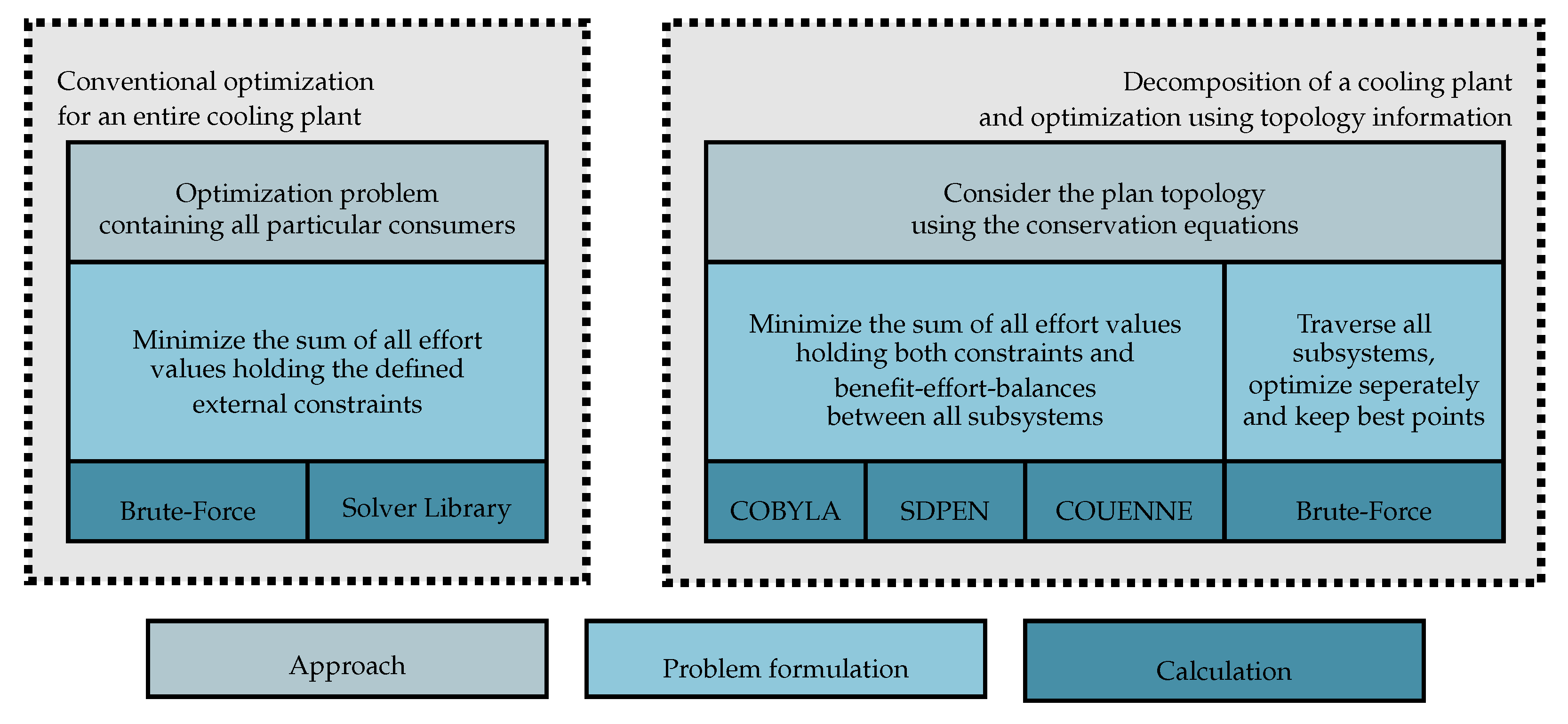
The established solvers cannot directly compute optimal set-points for the cooling plant. Figure 2 illustrates the different ways to address this problem. In a naive approach, one can just tune all adjustable parameters and observe the effect on the overall efficiency, either by brute-force search or using a solver. On the right in Figure 2, two categories of how to involve topology knowledge are mentioned. The first problem formulation combines all particular (primary) effort variables into an objective function and incorporates constraints which formalize the energy conservation law in every energy flow from one subsystem to another. Still, an overall optimization problem is solved completely.Here, without the decomposition to a graph, there are no intermediate efforts like cooling power transferred between the cooling tower and cooling water. The objective function holds the sum of all terms of primary consumption, e.g., the electrical energy demanded by pumps, fans, and compressors, which corresponds to the common root source of the OptTopo graph. In contrast, OptTopo decomposes the system, and finds solutions for every subsystem with respect to common efficiency.

4.2. Experimental Setup

In this section, we present the experiments conducted to evaluate OptTopo. We designed three different experiments: In the first experiment in Section 4.3.1 the general feasibility of the approach is demonstrated and in Section 4.3.2 the quality of its solutions is compared to the comparison and benchmarking algorithms COBYLA, SDPEN, and COUENNE. The last experiment in Section 4.3.3 examines the effect of a variation of the problem size on the optimizer.

The objective of the experimental optimization is to minimize the effort needed to deliver a specified cooling power to a consumer.

Table 1. Nomenclature of EnPI: Adjustable parameters $\phi$ and arbitrary but fixed parameters $\xi$.

Variable	Meaning
${\phi }_{\mathrm{TempCoTo}}$	set-point temperature for the cooling tower (CoTo)
${\phi }_{\mathrm{HysteresisA}}$, ${\phi }_{\mathrm{HysteresisB}}$	hysteresis width of the two chillers
${\phi }_{\mathrm{SetPressureCoW}}$	set pressure for the cooling water (CoW) cycle
${\phi }_{\mathrm{SetPressureChWa}}$	set pressure for the chilled water (ChWa) cycle
${\xi }_{\mathrm{TempHeatex}}$	temperature level between the cooling water cycle and the chillers
${\xi }_{\mathrm{TempConsumer}}$	temperature of the consumer

lists the relevant variables of the cooling plant. The assignment to the respective subsystems can be seen in Table 2. While all free parameters $\phi$ are adjustable, the temperature levels of the consumer and the heat exchanger, ${\xi }_{\mathrm{TempConsumer}}$ and ${\xi }_{\mathrm{TempHeatex}}$, depending on the entire system. As arbitrary but fixed parameters, they are used to ensure the compatibility of adjacent subsystems.Accordingly, the polynomial model in Equation (1) map from the free variables, external variables, and the arbitrary but fixed parameters to the efforts, benefits, and internal parameters. These static models were instanced using the MATLAB System Identification toolbox.

In Table 2, we can observe how the model of the given industrial system could be reduced by decomposition. For the decomposed system, the greatest amount of dimensions results for the modeling of the chillers, depending on four parameters. Since the subsystems are computed independently and sequentially, the dimension of the decomposed system equals the maximal dimension of a subsystem, which is four in this example. Analogous modeling of the overall system would depend on at least five dimensions, the free parameters $\mathrm{\Phi }$. The problem size could hence be reduced by one dimension.

Table 2. Overview of variables for each subsystem: While optimizing the entire system evokes a problem with five free influence variables, decomposing the entire system reduces to a maximum number of four dimensions to be considered from free variables $\mathrm{\Phi }$ and arbitrary but fixed variables $\mathrm{\Xi }$.

	Cooling Tower	Cooling Water	Chillers	Chilled Water	$\Sigma$
$\mathrm{\Phi }$	${\phi }_{\mathrm{TempCoTo}}$	${\phi }_{\mathrm{SetPressureCoW}}$	${\phi }_{\mathrm{HysteresisA}}$, ${\phi }_{\mathrm{HysteresisB}}$	${\phi }_{\mathrm{SetPressureChWa}}$	5
$\mathrm{\Xi }$	${\xi }_{\mathrm{TempHeatex}}$	${\xi }_{\mathrm{TempHeatex}}$	${\xi }_{\mathrm{TempHeatex}}$, ${\xi }_{\mathrm{TempConsumer}}$	${\xi }_{\mathrm{TempConsumer}}$	2
$\mathrm{\Sigma }$	2	2	4	2

Table 2. Overview of variables for each subsystem: While optimizing the entire system evokes a problem with five free influence variables, decomposing the entire system reduces to a maximum number of four dimensions to be considered from free variables $\mathrm{\Phi }$ and arbitrary but fixed variables $\mathrm{\Xi }$.

	Cooling Tower	Cooling Water	Chillers	Chilled Water	$\Sigma$
$\mathrm{\Phi }$	${\phi }_{\mathrm{TempCoTo}}$	${\phi }_{\mathrm{SetPressureCoW}}$	${\phi }_{\mathrm{HysteresisA}}$, ${\phi }_{\mathrm{HysteresisB}}$	${\phi }_{\mathrm{SetPressureChWa}}$	5
$\mathrm{\Xi }$	${\xi }_{\mathrm{TempHeatex}}$	${\xi }_{\mathrm{TempHeatex}}$	${\xi }_{\mathrm{TempHeatex}}$, ${\xi }_{\mathrm{TempConsumer}}$	${\xi }_{\mathrm{TempConsumer}}$	2
$\mathrm{\Sigma }$	2	2	4	2

4.3. Results and Interpretation

4.3.1. Feasibility of the Approach

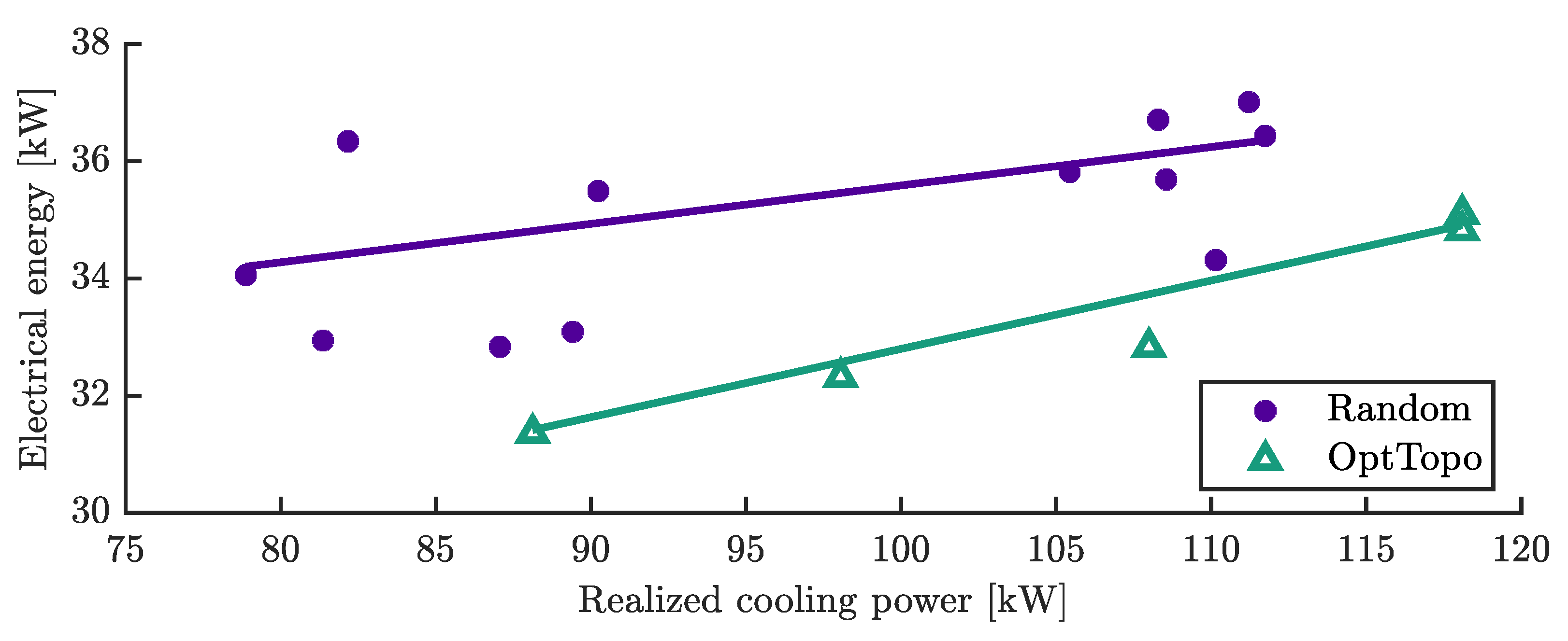
This experiment demonstrates the general functionality of the approach and the usability of the generated solutions. OptTopo is configured to optimize the described cooling system for five different requests equally distributed over the interval from 74 kW to 121 kW, see

Table 3. Five intervals of cooling power are defined as requests to the overall system.

$\mathrm{\nu }$

(74, 83.4]

(83.39, 92.8]

(92.8, 102.2]

(102.2, 111.6]

(111.6, 121]

. Afterward, the solutions are realized using the simulation of the system to demonstrate the feasibility and to compare their efficiency with randomly generated points. For this configuration, OptTopo needs approximately one hour, during which it executes ten billion function calls. There is no solution found for the lowest request. For the last request, however, OptTopo returned two solutions. This can occur if the predicted effort is (approximately) equal, in which case the selection of the optimal configuration should be based on a different operation criterion. Figure 3 illustrates that OptTopo achieves valid set-points, which lead to more efficient operating points in comparison to random settings meeting the same requested cooling power.

4.3.2. Comparison to Other Optimization Procedures

To evaluate the performance of the here presented algorithm OptTopo and the efficiency of its returned solutions beyond its general feasibility, the following experiment compares it to the benchmark algorithms COBYLA, SDPEN, and COUENNE. The amount and the interval of requests posed are the same as in the first experiment listed in the previous Section 4.3.1.

For the lowest request, the other optimizers also fail to find a solution, hinting at an error in the model, which renders this point infeasible. In addition, COBYLA does not find a solution for the second request. SDPEN and COUENNE, like OptTopo, find a solution for all the remaining four requests. For a demand of 102.2 kW to 111.6 kW, OptTopo returns the settings listed in

Table 4. For the interval request with an average value of $106.9$ kW, OptTopo provides the following values for the setpoint pressure at the chilled water, the hysteresis widths, the setpoint pressure at the cooling water, and the setpoint temperature at the cooling tower.

Variable	${\mathit{\phi }}_{\mathbf{SetPressureChWa}}$	${\mathit{\phi }}_{\mathbf{HysteresisA}}$	${\mathit{\phi }}_{\mathbf{HysteresisB}}$	${\mathit{\phi }}_{\mathbf{SetPressureCoW}}$	${\mathit{\phi }}_{\mathbf{TempCoTo}}$
Value	$1.66$ bar	$2.15$$\mathrm{K}$	$2.65$$\mathrm{K}$	$1.72$ bar	$21.05$${}^{°}\mathrm{C}$

. This interval is defined in the fixed grid with the center point 106.9 kW.

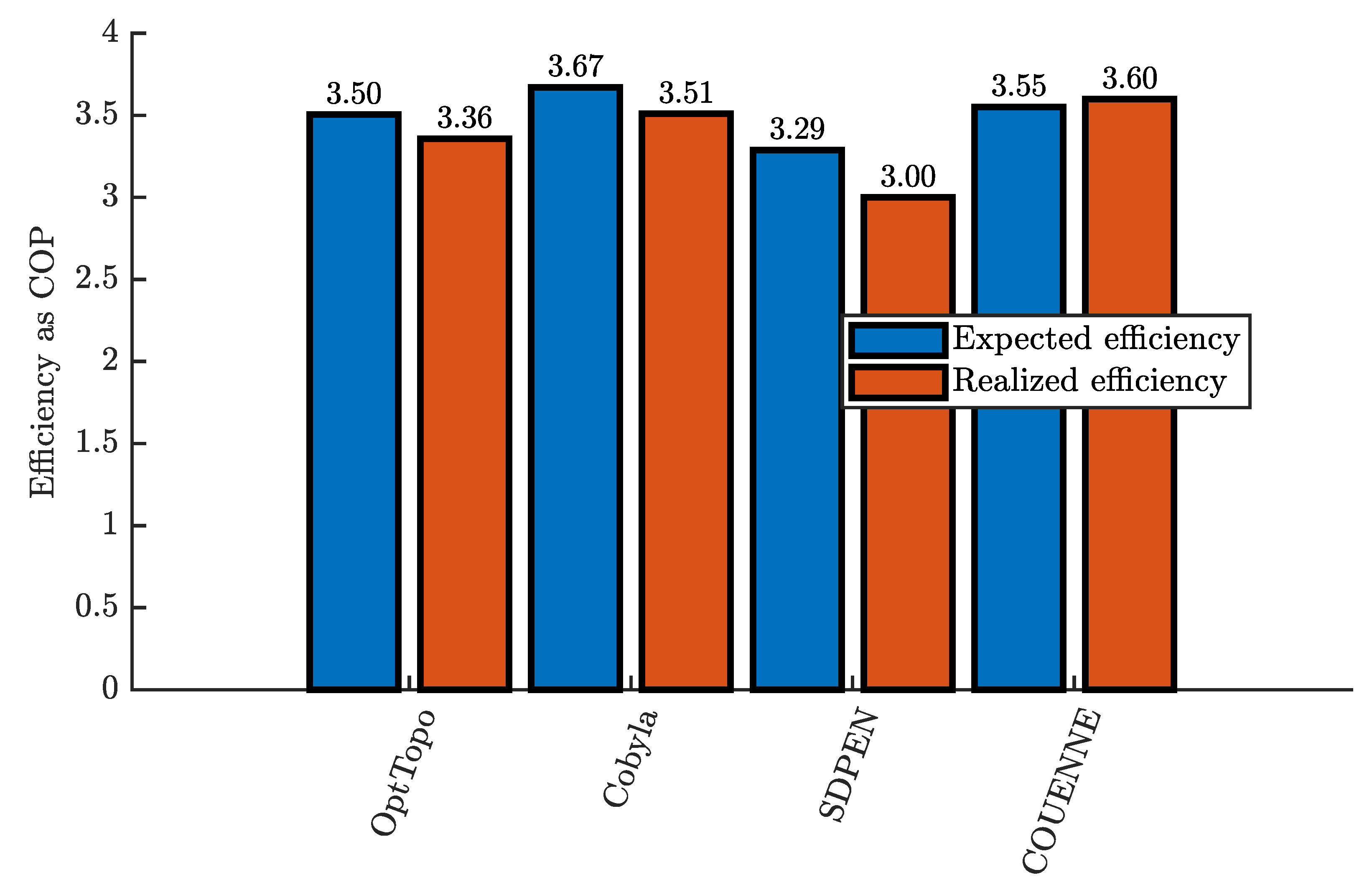
For cooling technology, the efficiency can be quantified using the Coefficient of Performance (COP) which gives the ratio of transported thermal power and electrical power used. Figure 4 shows the expected efficiency (blue, computed by the optimizer) and the realized efficiency (red, running the simulation with the returned solution) for one exemplary chosen request for all the optimizers. As expected, the global solver COUENNE reaches the best value. The remaining deviation may be caused by the model fit. For comparison, the efficiency achieved by COUENNE is assigned to 100% for better comparability. COBYLA and OptTopo accomplish $97.5$% and $97.2$% while SDPEN reaches 83%. In particular, SDPEN also displays the largest discrepancy between the expected and realized efficiency. For COUENNE, there is only a small difference between these values (being the only algorithm that underestimates the efficiency of its solution), while COBYLA and OptTopo both slightly overestimate their efficiency. The good (realized) result of the benchmark algorithm COUENNE yields a strong case for the suitability of the identified polynomials. In terms of efficiency, the first prototype of OptTopo deployed here seems to be able to compete successfully with the local solvers COBYLA and SDPEN.

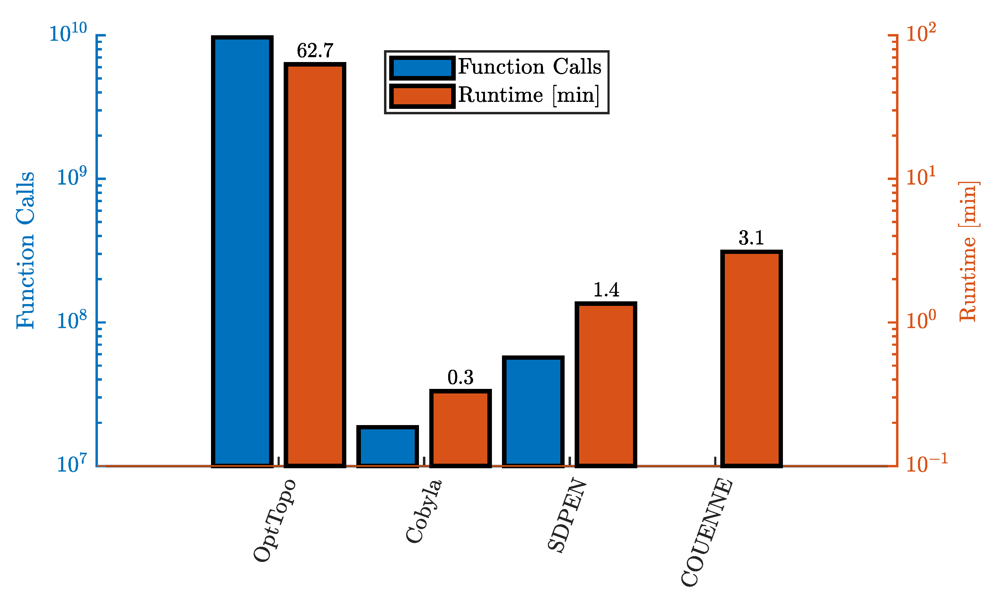
Figure 5 compares the runtime and number of function calls in this experiment for all the optimizers. Clearly, OptTopo is much more expensive than the other approaches. This high complexity is caused by the brute-force search utilized, which leads to a comparatively large number of function calls. As already stated in Section 3, this needs to be optimized via better-suited data structures and methodologies like parallelization not yet realized in this first prototype version of the algorithm. However, we stress again that OptTopo does not require additional computation time if queried with new requests from the same interval, whereas all the benchmark algorithms do.

4.3.3. Scalability

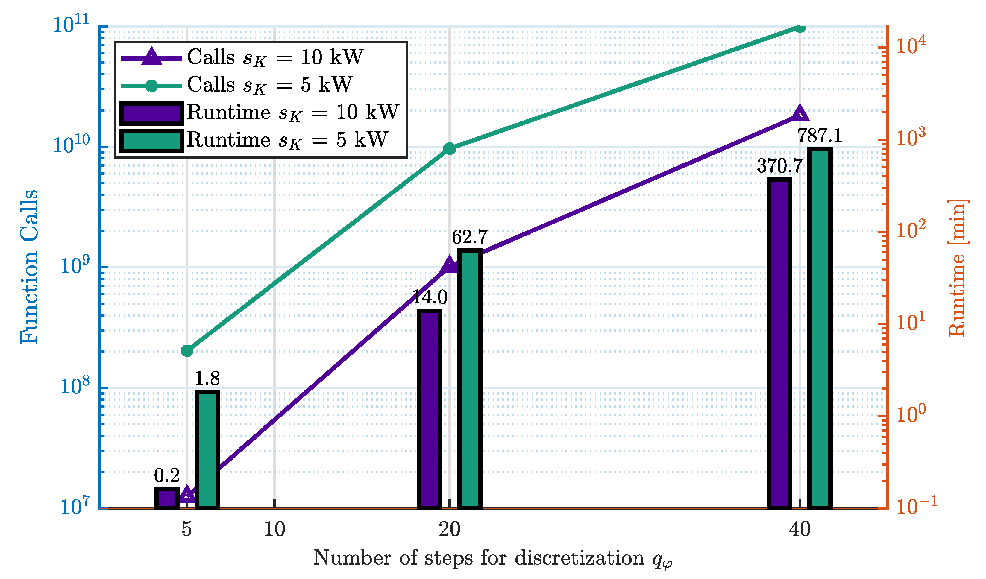
In this last experiment, the scalability of the approach is examined. In the current implementation, OptTopo uses a brute-force search to compute the optimal solutions of the subsystems. In doing so, the parameters of the model function have to be discretized in a suitable manner. More precisely, OptTopo is based on a fixed grid with free variables $\mathrm{\Phi }$ and arbitrary but fixed variables $\mathrm{\Xi }$ as independent dimensions. The number of discretization points is the same for all these dimensions, and we denote it by $q_{\phi }$. Besides that, the energy flows need to be discretized as described in Section 3. For this discretization, we tested only two different settings: A coarse discretization and a finer one. The flow of cooling power is discretized in steps of $s_K=5 \mathrm{k}\mathrm{W}$ or $s_K=10 \mathrm{k}\mathrm{W}$. This setting implies for $s_K=5 \mathrm{k}\mathrm{W}$ a fine discretization of the electrical power in 1 $\mathrm{k}$$\mathrm{W}$ steps and for $s_K=10 \mathrm{k}\mathrm{W}$ a coarser discretization of the electrical power in 2 $\mathrm{k}$$\mathrm{W}$ steps. For each of these two settings, Figure 6 plots the runtime of OptTopo over the granularity of $\mathrm{\Phi }$ and $\mathrm{\Xi }$ with $q_{\phi }$ = 5, 20 and 40.

As expected, both runtime and number of function calls grow with a finer discretization for the energy flows (purple versus green columns) and also with a finer discretization of the parameters (x-axis of the plot). This relation is also displayed in

Table 5. Runtime of OptTopo depending on the discretization: The computational effort increases with the number of steps in the grid, but this increase is slower than the expected exponential growth.

	Combinations	Function Calls	Runtime in Min
5 Steps	625	2.03e8	1.8395
Factor	256	47.6512	34.0853
20 Steps	16 × 104	9.6732 × 109	62.7
Factor	16	10.2292	12.5534
40 Steps	256 × 105	9.8949 × 1010	787.1

: The grid has a size of $q_{\phi }^{|\mathrm{\Phi }\cup \mathrm{\Xi }|}$ since all $|\mathrm{\Phi }\cup \mathrm{\Xi }|$ dimensions considered are divided into $q_{\phi }$ steps. In the presented use-case, the maximal number of dimensions is given by $|\mathrm{\Phi }\cap \mathrm{\Xi }|=4$ for the chillers (see Table 2). Thus, for ${\tilde{q}}_{\phi }=2·q_{\phi }$, the size of the grid grows to ${\tilde{q}}_{\phi }^{|\mathrm{\Phi }\cap \mathrm{\Xi }|}$ by a factor $2^4=16$. Table 5 shows that the number of function calls increases by a factor 10 instead of 16 when changing from 20 to 40 steps. In addition, when changing from 5 to 20 steps, the amount of combinations grows by factor 256, but the amount of function calls only by a factor of approximately 50. This effect is achieved by the component-wise optimization that allows discarding infeasible and non-efficient solutions for equal benefits at an early stage of the graph traversal so that not all of the possible combinations have to be saved.

5. Conclusions and Outlook

We presented a set-point optimization algorithm, OptTopo, which utilizes topological information from a complex system consisting of several subsystems connected by directed energy flows. We demonstrated OptTopo’s performance in comparison to widely used local solvers SDPEN and COBYLA, as well as the global solver COUENNE. While the presented prototype is prone to high complexity due to the brute-force search of the subsystem optimization, it could be demonstrated to compete successfully with the aforementioned local solvers in terms of reliability and efficiency. Both OptTopo and Cobyla achieved about 97% of the efficiency hit by COUENNE. The conventional solvers take only a few minutes to serve five requests but OptTopo requires over 60 $\min$. However, once OptTopo has finished, an optimal configuration for any given request adhering to the requested discretization can be received by a simple look-up, generating no additional cost. This is a big advantage compared to other widely used optimizers.

The mitigation of OptTopo’s complexity is a conjecture for future work. In its present form, the algorithm does not use parallelization, which could greatly increase the speed of optimization in systems with multiple parallel branches. The present version also requires that all parameters be contained in finite intervals, which are then discretized for brute-force optimization of the subsystems, leading to an excess of function calls compared to other methods. More sophisticated continuous optimization methods for the subproblems, even hybrid versions with local solvers such as SDPEN or COBYLA, could be introduced for the subsystems to reduce the computational burden.

References

1. Thiele, G.; Clauss, R.; Krüger, J.; Heimann, O. Chiller System Simulation and Optimization. Available online: https://fordatis.fraunhofer.de/handle/fordatis/124 (accessed on 2 November 2022).
2. Thiele, G.; Heimann, O.; Grabowski, K.; Krüger, J. Framework for energy efficiency optimization of industrial systems based on the Control Layer Model. Procedia Manuf. 2019, 33, 414–421. [Google Scholar] [CrossRef]
3. Grabowski, K.; Kubin, K.; Ernst, C. Energiekennzahl-Methodik zur Überwachung und Bewertung von Anlagen in produzierenden Unternehmen. Energiewirtschaft Tagesfragen 2015, 65. [Google Scholar]
4. Thiele, G.; Clauß, R.; Johanni, T.; Krüger, J. Energy optimal set-points for coupled systems using their topology. In Proceedings of the 2020 7th International Conference on Control, Decision and Information Technologies (CoDIT), Prague, Czech Republic, 29 June–2 July 2020; pp. 1052–1057. [Google Scholar] [CrossRef]
5. Thiele, G.; Johanni, T.; Sommer, D.; Krüger, J. OptTopo: Automated set-point optimization for coupled systems using topology information. In Proceedings of the 2022 8th International Conference on Control, Decision and Information Technologies (CoDIT), Istanbul, Turkey, 17–20 May 2022; pp. 1052–1057. [Google Scholar]
6. Behrooz, F.; Mariun, N.; Marhaban, M.H.; Mohd Radzi, M.A.; Ramli, A.R. Review of Control Techniques for HVAC Systems—Nonlinearity Approaches Based on Fuzzy Cognitive Maps. Energies 2018, 11, 495. [Google Scholar] [CrossRef] [Green Version]
7. Komareji, M.; Stoustrup, J.; Rasmussen, H.; Bidstrup, N.; Svendsen, P.; Nielsen, F. Optimal Set-point Synthesis in HVAC Systems. In Proceedings of the American Control Conference, New York, NY, USA, 9–13 July 2007; pp. 5076–5081. [Google Scholar] [CrossRef]
8. Komareji, M.; Stoustrup, J.; Rasmussen, H.; Bidstrup, N.; Svendsen, P.; Nielsen, F. Simplified optimal control in HVAC systems. In Proceedings of the 2009 IEEE Control Applications, (CCA) Intelligent Control, (ISIC), St. Petersburg, Russia, 8–10 July 2009; pp. 1033–1038. [Google Scholar] [CrossRef]
9. Asad, H.S.; Yuen, R.K.K.; Huang, G. Multiplexed real-time optimization of HVAC systems with enhanced control stability. Appl. Energy 2017, 187, 640–651. [Google Scholar] [CrossRef]
10. Asad, H.S.; Yuen, R.K.K.; Huang, G. Degree of freedom based set-point reset scheme for HVAC real-time optimization. Energy Build. 2016, 128, 349–359. [Google Scholar] [CrossRef]
11. Asad, H.S.; Yuen, R.K.K.; Liu, J.; Wang, J. Adaptive modeling for reliability in optimal control of complex HVAC systems. Build. Simul. 2019, 12, 1095–1106. [Google Scholar] [CrossRef]
12. Mu, B.; Li, Y.; House, J.M.; Salsbury, T.I. Real-time optimization of a chilled water plant with parallel chillers based on extremum seeking control. Appl. Energy 2017, 208, 766–781. [Google Scholar] [CrossRef]
13. Tan, Y.; Li, Y.; Mareels, I.M.Y. Extremum Seeking for Constrained Inputs. IEEE Trans. Autom. Control. 2013, 58, 2405–2410. [Google Scholar] [CrossRef]
14. Zhao, Z.; Li, Y.; Salsbury, T.I.; House, J.M. Extremum-seeking control integrated online input selection with application to a chilled-water plant. Sci. Technol. Built Environ. 2022, 28, 170–187. [Google Scholar] [CrossRef]
15. Eberspächer, P.; Verl, A. Realizing Energy Reduction of Machine Tools Through a Control-integrated Consumption Graph-based Optimization Method. Procedia CIRP 2013, 7, 640–645. [Google Scholar] [CrossRef] [Green Version]
16. Schlechtendahl, J.; Eberspächer, P.; Schraml, P.; Verl, A.; Abele, E. Multi-level Energy Demand Optimizer System for Machine Tool Controls. Procedia CIRP 2016, 41, 783–788. [Google Scholar] [CrossRef]
17. Bakakeu, J.; Kisskalt, D.; Franke, J.; Baer, S.; Klos, H.H.; Peschke, J. Multi-Agent Reinforcement Learning for the Energy Optimization of Cyber-Physical Production Systems. In Proceedings of the 2020 IEEE Canadian Conference on Electrical and Computer Engineering (CCECE), London, ON, Canada, 30 August–2 September 2020; pp. 1–8. [Google Scholar]
18. Bakakeu, J.; Baer, S.; Klos, H.H.; Peschke, J.; Brossog, M.; Franke, J. Multi-Agent Reinforcement Learning for the Energy Optimization of Cyber-Physical Production Systems. In Artificial Intelligence in Industry 4.0: A Collection of Innovative Research Case-Studies that Are Reworking the Way We Look at Industry 4.0 Thanks to Artificial Intelligence; Springer: Berlin/Heidelberg, Germany, 2021; pp. 143–163. [Google Scholar]
19. Leibo, J.Z.; Hughes, E.; Lanctot, M.; Graepel, T. Autocurricula and the Emergence of Innovation from Social Interaction: A Manifesto for Multi-Agent Intelligence Research. arXiv 2019, arXiv:1903.00742. [Google Scholar]
20. Panten, N. Deep Reinforcement Learning zur Betriebsoptimierung hybrider industrieller Energienetze. Ph.D. Thesis, Technische Universität Darmstadt, Darmstadt, Germany, 2019. [Google Scholar]
21. Weigold, M.; Ranzau, H.; Schaumann, S.; Kohne, T.; Panten, N.; Abele, E. Method for the application of deep reinforcement learning for optimised control of industrial energy supply systems by the example of a central cooling system. CIRP Ann. 2021, 70, 17–20. [Google Scholar] [CrossRef]
22. Wang, X.; Zhao, Q.; Wang, Y. A Distributed Optimization Method for Energy Saving of Parallel-Connected Pumps in HVAC Systems. Energies 2020, 13, 3927. [Google Scholar] [CrossRef]
23. Wang, X.; Zhao, Q.; Wang, Y. An asynchronous distributed optimization method for energy saving of parallel-connected pumps in HVAC systems. Results Control. Optim. 2020, 1, 100001. [Google Scholar] [CrossRef]
24. Kahn, A.B. Topological Sorting of Large Networks. Commun. ACM 1962, 5, 558–562. [Google Scholar] [CrossRef]
25. Hart, W.E.; Watson, J.P.; Woodruff, D.L. Pyomo: Modeling and solving mathematical programs in Python. Math. Program. Comput. 2011, 3, 219–260. [Google Scholar] [CrossRef]
26. Perez, R.E.; Perez, R.E.; Jansen, P.W.; Jansen, P.W.; Martins, J.R.R.A.; Martins, J.R.R.A. pyOpt: A Python-based object-oriented framework for nonlinear constrained optimization. Struct. Multidiscip. Optim. 2012, 45, 101–118. [Google Scholar] [CrossRef]
27. Liuzzi, G.; Lucidi, S.; Sciandrone, M. Sequential Penalty Derivative-Free Methods for Nonlinear Constrained Optimization. SIAM J. Optim. 2010, 20, 2614–2635. [Google Scholar] [CrossRef]
28. Mangasarian, O.; Fromovitz, S. The Fritz John necessary optimality conditions in the presence of equality and inequality constraints. J. Math. Anal. Appl. 1967, 17, 37–47. [Google Scholar] [CrossRef] [Green Version]
29. Powell, M.J.D. A Direct Search Optimization Method That Models the Objective and Constraint Functions by Linear Interpolation. In Advances in Optimization and Numerical Analysis; Gomez, S., Hennart, J.P., Eds.; Springer: Dordrecht, The Netherlands, 1994; pp. 51–67. [Google Scholar]
30. Belotti, P.; Lee, J.; Liberti, L.; Margot, F.; Wächter, A. Branching and bounds tighteningtechniques for non-convex MINLP. Optim. Methods Softw. 2009, 24, 597–634. [Google Scholar] [CrossRef]
Figure 1. Schema of a typical cooling plant with assigned parameters.
Energies 15 08387 g001
Figure 2. This paper compares the approaches in the right box and does not deal with approaches that do not utilize the topology information.
Energies 15 08387 g002
Figure 3. Operation points resulting from solutions from OptTopo together with operation points from randomly chosen configurations. The former ones prove to realize a lower demand for electrical energy in this sample. A regression illustrates this trend.
Energies 15 08387 g003
Figure 4. Efficiency of the optimizers in comparison: The blue bars illustrate the efficiency which is claimed by the optimization algorithm and the red bars give the actual achieved efficiency.
Energies 15 08387 g004
Figure 5. The runtime of the optimizers in comparison: The logarithmic scale allows a better illustration. OptTopo is by far slower than the competitors.
Energies 15 08387 g005
Figure 6. Runtime of OptTopo for different numbers of discretization steps q φ : With a finer discretization, the runtime grows slower than exponentially.
Energies 15 08387 g006