Article

Solution of Probabilistic Optimal Power Flow Incorporating Renewable Energy Uncertainty Using a Novel Circle Search Algorithm

1
Electrical Engineering Department, Future University in Egypt, Cairo 11835, Egypt
2
State Key Laboratory of Advanced Electromagnetic Engineering and Technology, Huazhong University of Science and Technology, Wuhan 430074, China
3
Centre for Advances in Reliability and Safety, Hong Kong, China
4
Electrical Power and Machines Department, Faculty of Engineering, Ain Shams University, Cairo 11517, Egypt
5
Department of Mechanical Engineering, National University of Singapore, 9 Engineering Drive 1, Singapore 117576, Singapore
6
Department of Electrical Engineering, Superior Polytechnic School of Linares, University of Jaén, 23700 Linares, Spain
7
Electrical Power and Machines Engineering Department, Faculty of Engineering, Tanta University, Tanta 31511, Egypt
*
Author to whom correspondence should be addressed.
Energies 2022, 15(21), 8303; https://doi.org/10.3390/en15218303
Submission received: 8 October 2022 / Revised: 1 November 2022 / Accepted: 4 November 2022 / Published: 7 November 2022

Abstract

:
Integrating renewable energy sources (RESs) into modern electric power systems offers various techno-economic benefits. However, the inconsistent power profile of RES influences the power flow of the entire distribution network, so it is crucial to optimize the power flow in order to achieve stable and reliable operation. Therefore, this paper proposes a newly developed circle search algorithm (CSA) for the optimal solution of the probabilistic optimal power flow (OPF). Our research began with the development and evaluation of the proposed CSA. Firstly, we solved the OPF problem to achieve minimum generation fuel costs; this used the classical OPF. Then, the newly developed CSA method was used to deal with the probabilistic power flow problem effectively. The impact of the intermittency of solar and wind energy sources on the total generation costs was investigated. Variations in the system’s demands are also considered in the probabilistic OPF problem scenarios. The proposed method was verified by applying it to the IEEE 57-bus and the 118-bus test systems. This study’s main contributions are to test the newly developed CSA on the OPF problem to consider stochastic models of the RESs, providing probabilistic modes to represent the RESs. The robustness and efficiency of the proposed CSA in solving the probabilistic OPF problem are evaluated by comparing it with other methods, such as Genetic Algorithm (GA), Particle Swarm Optimization (PSO), and the hybrid machine learning and transient search algorithm (ML-TSO) under the same parameters. The comparative results showed that the proposed CSA is robust and applicable; as evidence, an observable decrease was obtained in the costs of the conventional generators’ operation, due to the penetration of renewable energy sources into the studied networks.

1. Introduction

Integrating RES, such as solar photovoltaic (PV) and wind turbine (WT) sources, into electric distribution networks has been emphasized in the last two decades, due to the advantages of low prices and an environmentally clean electric power supply. However, managing the intermittent profile of renewable energy sources (RESs) is challenging in terms of keeping the system operation smooth. Optimizing the power flow in electric distribution networks plays an important role. The optimal power flow (OPF) problem is a large-constrained multi-objective problem, wherein the main objectives are to reduce the fuel cost of power generation and reduce the losses of the transmission lines, considering the constraints of power generation and voltage variations [1,2,3]. The OPF for large power systems requires extensive data on the transmission line parameters, bus voltages, and power generation constraints [4]. The OPF problem can be solved as a single-objective or multi-objective function optimization problem [5]. Due to environmental protection considerations and the consequent changes in the structure of energy provision, there is a growing integration of renewable energy sources (RESs) with electrical power systems. RESs assure superiority in carbon emissions reduction. In addition, they are considered sustainable energy sources compared to conventional thermal power stations [6]. In the past, the OPF problem in its classical formulation was solved by deterministic methods [7,8]. After that, many classical optimization methods were introduced to solve the classical OPF problem [9]. However, the classical type of OPF problem did not include RES in the problem formulation [10]. Recently, the formulation of the OPF problem has been developed to consider RES in the power system [11]. The inclusion of RES in the OPF problem model led to uncertainties [12]. The uncertainties in the power systems need probabilistic models to deal with them [13,14]. Therefore, the probabilistic optimal power flow (POPF) problem appears [15,16]. The difference between the OPF and the POPF problems is that the POPF solution is determined based on probabilistic models instead of deterministic ones [17]. Therefore, this paper addresses the uncertainties of wind speed and solar irradiance by proposing statistical models to determine the generated power from such inserted RESs accurately [18,19].
The solutions available to the POPF problem can be classified as analytical [20,21], approximate [22], numerical [23], and heuristic approaches [24]. Error! Reference source not found.For example, the authors of [25] treat the POPF problem as a probabilistic inference model using Bayesian inference. Elsewhere, the authors of [26] provide a novel POPF model that copes with uncertainties, considering electrical power generation from a wind turbine. Another study [27] introduces a new POPF problem solution approach for electrical power networks, including wind energy sources, using an approach that adopts sampling to determine the probability density functions (PDF). The authors of [28] provide a new method for the POPF solution of large power networks, including Pearson correlated uncertainty sources, using a technique that enhances the efficiency from each aspect. Finally, reference [29] presents the incorporation of optimal DG allocation and network reconfiguration to improve voltage stability and reduce distribution network losses while considering probability in terms of loads at different power factors, using a modified version of the whale optimization method.
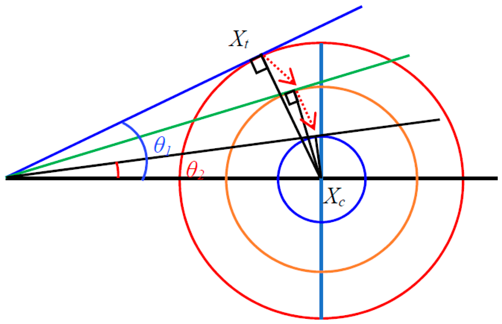
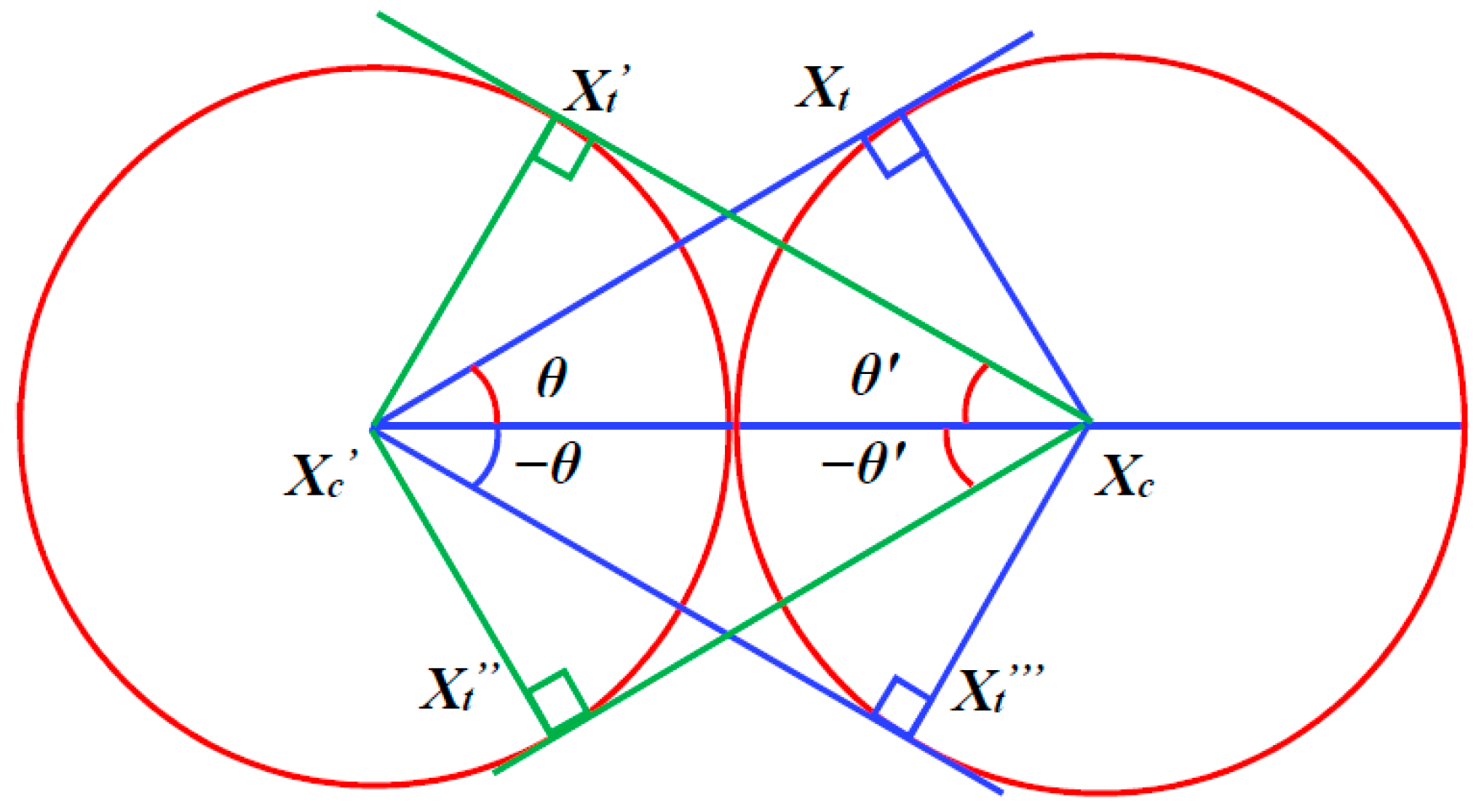
In this paper, the application of a novel algorithm, called the circle search algorithm (CSA) optimization method, for solving the POPF problem is introduced for the first time, to reach a global solution proficiently without becoming trapped in local minima, compared to other existing algorithms. The CSA algorithm was first introduced in 2022 by Mohammed H. Qais et al. [30]. The CSA optimization algorithm is classified as a geometry-based and metaheuristic optimization method. The category of geometry-based optimization methods also includes the sine-cosine optimization method. The sine-cosine optimization method simulates sinusoidal waveforms [31,32]. The inspiration for the CSA comes from the geometrical features of the circle. Geometry studies the features of the figures in space. The circle is a geometric shape that has a diameter, center, and circumference, as well as tangential lines. The radius length, divided by the tangent line length, represents the orthogonal function of the angle that opposes the orthogonal radius. Such an angle is vital to explore new search agents and is also important for the exploitation process of the proposed optimization algorithm. A small change in angle leads to a significant difference in orthogonal function. This can help accelerate the exploration behavior.
The significant contributions of the current article can be summarized as follows:
  • We are introducing a newly developed CSA to solve the OPF problem, as well as the POPF one.
  • We have reformulated the CSA optimization method for integrating RESs apart from fuel generators, with different scenarios and conditions reflecting system demands.
  • We have developed statistical models for the RESs, depending on actual historical measurements. The provided models can help to accurately determine the amount of electrical power that is generated, while solving the POPF problem.
  • We have evaluated the efficiency of the CSA optimization method using MATLAB software, applied to the IEEE 57-bus test system and the 118-bus system. The introduced method is further validated with the commonly used algorithms of Genetic Algorithm (GA), and the Particle Swarm Optimization (PSO).
The remainder of the article is divided as follows: Section 2 introduces the objective mathematical formulation; Section 3 presents the modeling of the WT and PV; the CSA is provided in Section 4. Section 5 shows the results and analysis; Section 6 offers the authors’ conclusions.

2. Problem Formulation

In the first stage, the CSA optimization method is used to get the solution to the classical case of the OPF problem. The fitness function in this stage minimizes the cost of the power generated from conventional generators. In the second stage, the CSA is adapted to solve the POPF problem, considering the randomness of both the irradiance and the wind speed, which correspondingly affects the output of power generated from the solar PV panels and WTs.

2.1. The Classical Optimal Power Flow Problem

This section introduces the solution to the OPF problem of the IEEE 57-bus and IEEE 118-bus test systems, assuming constant loads and that the power generation comes only from conventional generation methods [33]. The cost of power generation, which represents the objective function, is described mathematically in the following subsections [34].

2.1.1. The Cost Function

The calculation of the total generation cost is shown in Equation (1). As seen, the total cost is calculated by summing the generation costs of the generators. The equation of the cost of such generation is shown in Equation (2). The cost of the power per generator is mathematically defined as a quadratic equation of the real power [35]:
M i n i m i z e               J = h = 1 24 i = 1 N G C i , h ( P G i , h )
C i , h ( P G i , h ) = a i * P G i , h 2 + b i * P G i , h + c i
where J is the total cost, N G is the number of generators, and P G i , h is the real power generated at location ‘ i ’ at hour ‘ h ’. In the second part of the study, where the POPF problem is performed, the cost function is recalculated independently at each hour.

2.1.2. The Optimization Problem Constraints

The proposed optimization problem’s limitations can be divided into equality and inequality constraints. The equality constraints are constraints on the active and reactive powers. There are also equality constraints on the power transmitted through the OHTLs, due to thermal considerations. The equality constraints are mathematically represented in Equations (3), (4) and (8). Conversely, inequality limitations represent the constraints on the active and reactive power of the generators. Moreover, there are minimum and maximum restrictions on the bus voltages. The inequality constraints are mathematically represented by Equations (5)–(7) [36]:
P i n j k , h V k , h l = 1 N V l , h * [ G k l * cos ( δ k , h δ l , h ) + B k l * sin ( δ k , h δ l , h ) ] = 0
Q i n j k , h V k , h l = 1 N V l , h * [ G k l * sin ( δ k , h δ l , h ) B k l * cos ( δ k , h δ l , h ) ] = 0
where P i n j k , h and Q i n j k , h are the active and reactive powers at bus ‘ k ’. V k , h and V l , h are the bus voltages at hour ‘ h ’. G k l is the conductance, B k l is the susceptance, and δ l , h is the voltage angle:
P G m i n P G i , h P G m a x   ,   i = 1 , 2 , ,   N G   a n d   h = 1 , 2 , , 24
Q G m i n Q G i , h Q G m a x   ,   i = 1 , 2 , ,   N G   a n d   h = 1 , 2 , , 24
V i m i n V i , h V i m a x   ,   i = 1 , 2 , ,   N G   a n d   h = 1 , 2 , , 24
| V k , h * V l , h * [ G k l * cos ( δ l , h δ k , h ) + B k l * sin ( δ l , h δ k , h ) ] | P l i m k l ,   k , l = 1 , 2 , , N
where P G m i n and Q G m i n are the minimum power of the generator, P G m a x and Q G m a x are the maximum power of the generator, and P l i m k l is the maximum power of the OHTL between buses ‘ k ’ and ‘ l ’.
The newly developed CSA optimization method suggests candidate populations that satisfy the constraints stated in Equation (5). The objective function of Equation (2) is modified by adding terms as penalty factors, to force the solutions to remain within their limits. The penalties are mathematically expressed as follows:
Penalties = K v i = 1 N [ max ( 0 , V i V i m a x ) + max ( 0 , V i m i n V i ) ] + K l j = 1 n b r [ max ( 0 , S a j S a j r a t e d ) ]
where K v and K l are constants equal to 9 × 10 15 and 9 × 10 13 . S a is the power through branch ‘ j ’, and S a j r a t e d represents its limit.
MATLAB software was used to perform the optimization problem of this study, including the MATPOWER library for power systems. The CPU specification used in this study is “up to 8th Generation Intel® Quad Core i7-8550U”.

2.2. The POPF Problem

In this subsection, the problem is modified to include the stochastic nature of the RESs in the system [37,38,39]. In addition, the power systems’ loads are considered variable throughout the day [40]. This section investigates the effect of inserting the RESs into the system and how the generation costs are affected. Four scenarios depicting the optimization problem are studied in this section. In scenario 1, the loads of the power systems are changed throughout the daylight hours, while there are no RESs inserted. The POPF is solved every hour independently. In scenario 2, the power generation from PV panels, with their probabilistic models of solar irradiance, is added to the systems to investigate the effect on the generation costs of the fuel generators. The POPF problem is then solved hourly. In scenario 3, the power generated from the wind turbine is added to the systems, to share the burden of the conventional generators and to reduce the overall power production costs. The POPF is then repeated independently. In scenario 4, the POPF is solved, considering the stochastic nature of the power generated from both types of RESs (solar PV and WT). The integration of the RESs with their probabilistic models makes the optimization problem more complex. The probabilistic model of power generated from the wind turbine is constructed, based on six readings of wind speed per hour. Similarly, the probabilistic model of power generated from the PV panels is built based on sixty readings of solar irradiance per hour.

3. Modeling of Renewable Energy Uncertainty

Electrical power generation from PV array and WT farm is highly uncertain and is affected by solar irradiance and wind speeds [41,42,43,44]. Accordingly, the accurate modeling of the generators of the PV panels and the wind turbine is essential. The following sections present further details about such models.

Solar PV Power Generator

Depending on the solar irradiance ( S ) , the electrical power generated from the PV array is mathematically represented as in Equation (10) [45]:
P P V ( S ) = { P p v n S 2 S s t c R c                     f o r   S < R c P p v n S S s t c                               f o r   S R c .
where P p v n is the nominal power, S s t c is the standard conditions for irradiance, and R c is a certain irradiance point.
The Beta probability density function f s ( S ) is used to model the irradiance. Thus, it is mathematically expressed in Equation (11):
f s ( S ) = { Γ ( α + β ) Γ ( α ) Γ ( β ) × S ( α + 1 ) × ( 1 S ) ( β 1 ) ,               f o r   0 S 1 , α 0 , β 0 0 ,                                                                                                                                                                                   o t h e r w i s e .
The unit of ‘ S ’ is kW/m2. ‘ α ’ and ‘ β ’ are the shape parameters of the used probability density function. ‘ Γ ’ denotes the Gamma function. The ‘ α ’ and ‘ β ’ are determined during a time period, ‘ h ’, as in Equations (12) and (13):
β h = ( 1 μ s h ) × ( μ s h ( 1 + μ s h ) ( σ s h ) 2 1 )
α h = μ s h × β h ( 1 μ s h ) .
The number of samples for the Beta function N s . The power generated is forecasted and calculated as shown in Equation (14).
P P V = g = 1 N s P P V g × f s ( S g h ) g = 1 N s f s ( S g h )
where S g h is the solar irradiance, and f s ( S g h ) is its probability.
According to the wind blow, the power generated is a function of wind speed, and it is calculated as shown in Equation (15) [45]:
P W T ( v ) = { 0                                                                                   v v c i v v c i v n v c i × P w t n                     v c i < v v n P w t n                                                   v n < v v c o 0                                                                                   v v c o
where P w t n is the nominal WT power, v n is the nominal wind speed, v c i is the cut-in wind speed, and v c o is the cut-off wind speed. The modeling of the wind speed follows the Weibull PDF f v ( v ) , which is calculated, as shown in Equation (16):
f v ( v ) = k C × ( v C ) k 1 × e ( v C ) k
where C and k are the scale parameter and shape parameter of the Weibull probability density function. r is a uniform random number, the range of which is [0, 1]. The parameters, C , and k , are obtained from ( μ v h ) , and ( σ v h ) . ( μ v h ) and ( σ v h ) are the mean and the standard deviation of the speeds. They are calculated as shown in Equations (17) and (18):
k h = ( σ v h μ v h ) 1.086
C h = μ v h Γ ( 1 + 1 k h ) .
N v is the number of samples of the Weibull distribution function. The corresponding probabilistic speeds are used to determine the forecasted generated powers. The predicted power generated from the WT is mathematically represented, as in Equation (19):
P W T = g = 1 N v P W T g × f v ( v g h ) g = 1 N v f v ( v g h )
where v g h is the wind speed and f v ( v g h ) is its probability.

4. Proposed Solution Method

A novel competitive optimization algorithm, CSA, is introduced in this manuscript for the POPF simulation.

4.1. Background

A circle is a closed path featured by an equal distance from any point to its center. The diameter of the circle is measured as the distance between any two points on the circle and passes through its center ( x c ). The radius ( R ) of the circle is the distance from a point on the circle to its center. A tangent to the circle is defined as a line that intersects the circle at a single point ( x t ) at which the radius and the tangent are perpendicular.

4.2. The Circle Search Algorithm Formulation

The CSA optimization algorithm explores the optimal solution within random circles. Targeting the circle center, the angle θ decreases upon reaching the circle’s center. Figure 1 shows the decrease in the angle θ .
To prevent trapping at a local minimum, the angle θ is changed randomly. Figure 2 is provided for more clarity. Point x t defines the population of the CSA optimization algorithm. Meanwhile, x c defines the optimal solution of the CSA. The CSA optimization algorithm updates the population corresponding to moving x t in the direction of x c .
The main procedures of the CSA optimization algorithm are explained as follows:
(1)
Initialize the first population randomly between the upper and lower limits of the design variables.
(2)
Step 2: Update the population ( X t ) based on the calculated X c as presented mathematically in Equation (20):
X t = X c + ( X c X t ) × tan ( θ ) .
The angle θ has a significant effect on the exploration and exploitation phases. The calculation of the angle θ is mathematically represented as follows:
θ = { w × r a n d         I t e r > ( c × M a x i t e r )       ( e s c a p e   f r o m   l o c a l   s t a g n a t i o n ) w × p                                                                                                                                                                               o t h e r w i s e
w = w × r a n d w
a = π π × ( I t e r M a x i t e r ) 2
p = 1 0.9 × ( I t e r M a x i t e r ) 0.5
where the range of ‘ r a n d ’ is [0, 1]. I t e r is the number of the current iteration, and ‘ c ’ is a constant where the range is [0, 1] and refers to the percentage of maximum iterations. ‘ w ’ moves from π to 0 upon the increase in the iteration number. ‘ a ’ moves from π toward 0, depending on Equation (23). ‘ p ’ changes from 1 to 0, based on Equation (24). Consequently, the angle θ moves from π towards 0 . When the iteration number is greater than ( c × M a x i t e r ) , the angle θ equals w × r a n d .   The exploration phase is then improved. On the other hand, when the iteration is less than ( c × M a x i t e r ) , the angle θ   equals   w × p . Accordingly, the exploitation phase is improved. The populations of the CSA are further improved by applying the levy function [46], which can be represented as follows:
L F ( γ ) = 0.01 × u × σ | v | 1 γ   , σ = ( Γ ( 1 + γ ) × sin ( π γ 2 ) Γ ( 1 + γ 2 ) × γ × 2 ( γ 1 2 ) ) 1 γ
where v and u are random numbers in the range of [0, 1]. ‘ L F ’ is the levy function factor.
Figure 3 provides the flowchart for solving the OPF/POPF problems using the proposed improved CSA.

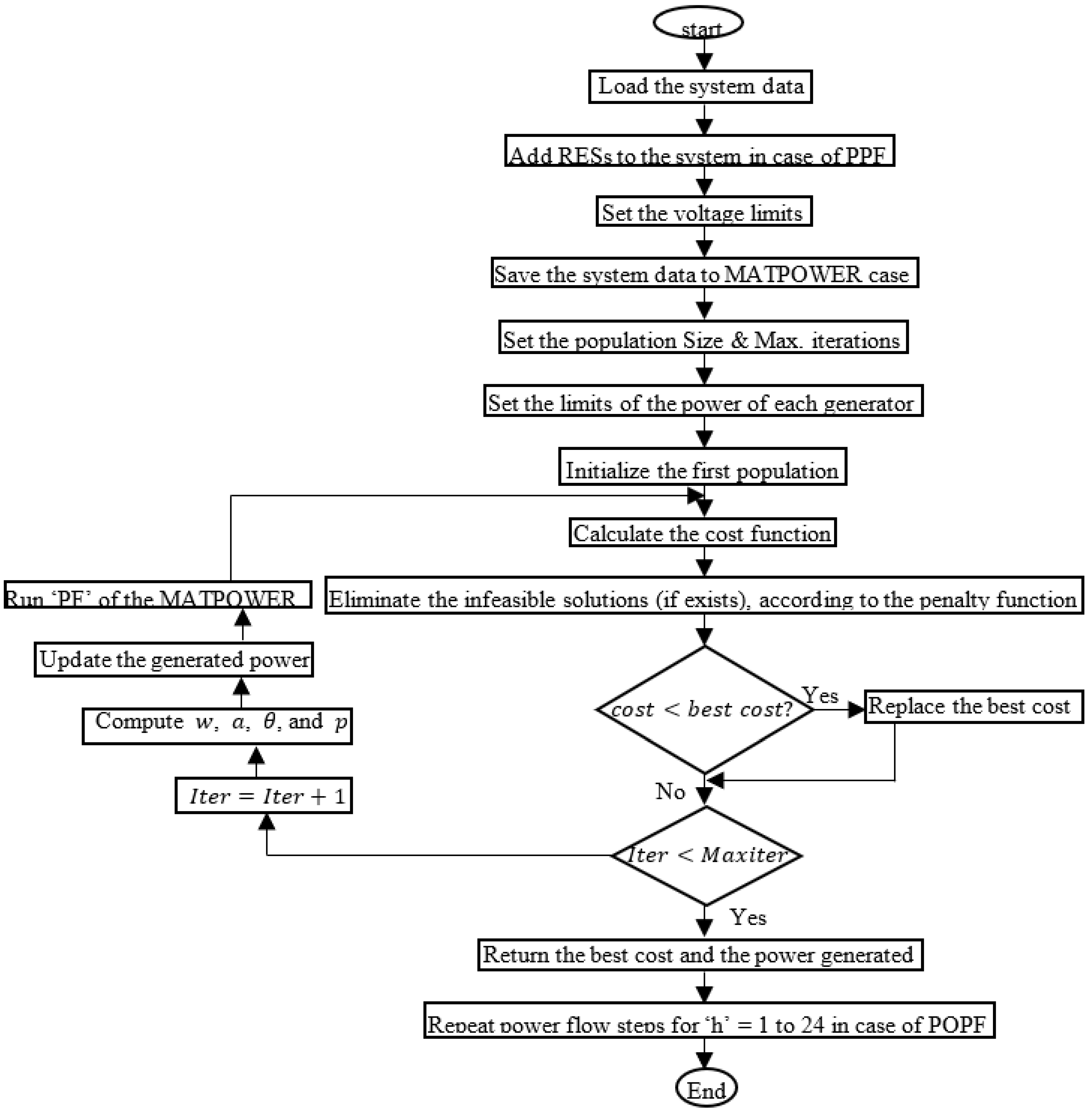
5. Analysis of the Simulation Results

The discussion and analysis of the simulation results are presented in this section. First, the simulation results of the classical OPF optimization problem are shown, compared, and analyzed. The classical OPF optimization problem itself is a well-established optimization problem, but in this paper, the performance of the newly developed and enhanced CSA method is evaluated by solving the OPF problem in its classical formulation. The comparisons and analyses of the simulation results are used in other optimization algorithms. Some of these optimization algorithms are well established, such as the GA and the PSO. Other recently published optimization algorithms are included in results comparisons, such as hybrid machine learning with transient search optimization (ML-TSO). These comparisons are presented to test how competitive the CSA algorithm is in solving such optimization problems. For more validation of the enhanced CSA method, more than one standard test system is used in the test, such as the IEEE 57-bus system and the IEEE 118-bus system.
The POPF problem simulation results are presented and discussed In the second section, where the PV array and the WT farm are inserted into the studied system in different scenarios, considering their stochastic nature. In this part of the study, the loads on the systems are also time-varying. The increasing penetration of the RESs made it important to consider the model of the photovoltaic systems and the wind energy systems with their stochastic nature in the OPF problem, to achieve optimal operating conditions in the electrical power systems. Integrating the RESs into the studied systems significantly affected the generation costs. This is also shown in detail in Section 5.1.2 and Section 5.2.2.
At the end of the Section 5, statistical analysis and the numerical results of the classical OPF problem are provided. The statistical analysis measures how robust the CSA model is. The essential data regarding the specification of the two standard systems used in the study are provided in Table 1.
The mutation operator of the GA optimization method is selected as 10%, while the crossover operator is selected as 65%. A conventional GA is used, which is based on uniform distribution selection. The search agents’ size is 15. Conversely, the inertia coefficient of the PSO algorithm is chosen as ‘1’. The inertia coefficient damping ratio equals 0.99. Meanwhile, the personal and social acceleration coefficients equal 2. The population size is 15. In the case of the CSA, the population size is 40.

5.1. First Test System: The IEEE 57-Bus Test Network

5.1.1. The Classical OPF Results

To verify the simulation results achieved by the proposed CSA algorithm, the same optimization problem was tackled using the GA, ML-TSO algorithm and the PSO. The stopping criterion of the compared optimization methods’ simulation process is 600 iterations. The simulation results of the classical are then compared and shown in Table 2. The design variables are also included in the tables. The control parameters are the active power generated by fuel generators. Figure 4 offers a more graphical comparison between the convergence performance of the CSA, the GA, the ML-TSO, and the PSO in the IEEE 57-bus test system. In this figure, a focus in the last three iterations is also shown.
It can be seen from the previous figure that the CSA reached its best solution at the end of the iterations. The CSA needed fewer than 100 iterations to gain a better solution than the GA and the PSO. After 600 iterations, the proposed CSA optimization algorithm achieved superior simulation results than the GA, by 0.044079%, and outstanding simulation results compared to the PSO results, by 0.9306%. Comparing the ML-TSO with the proposed CSA, it is clear that they reached almost the same optimization results.

5.1.2. The POPF with RESs Uncertainties and Load Demand Variation

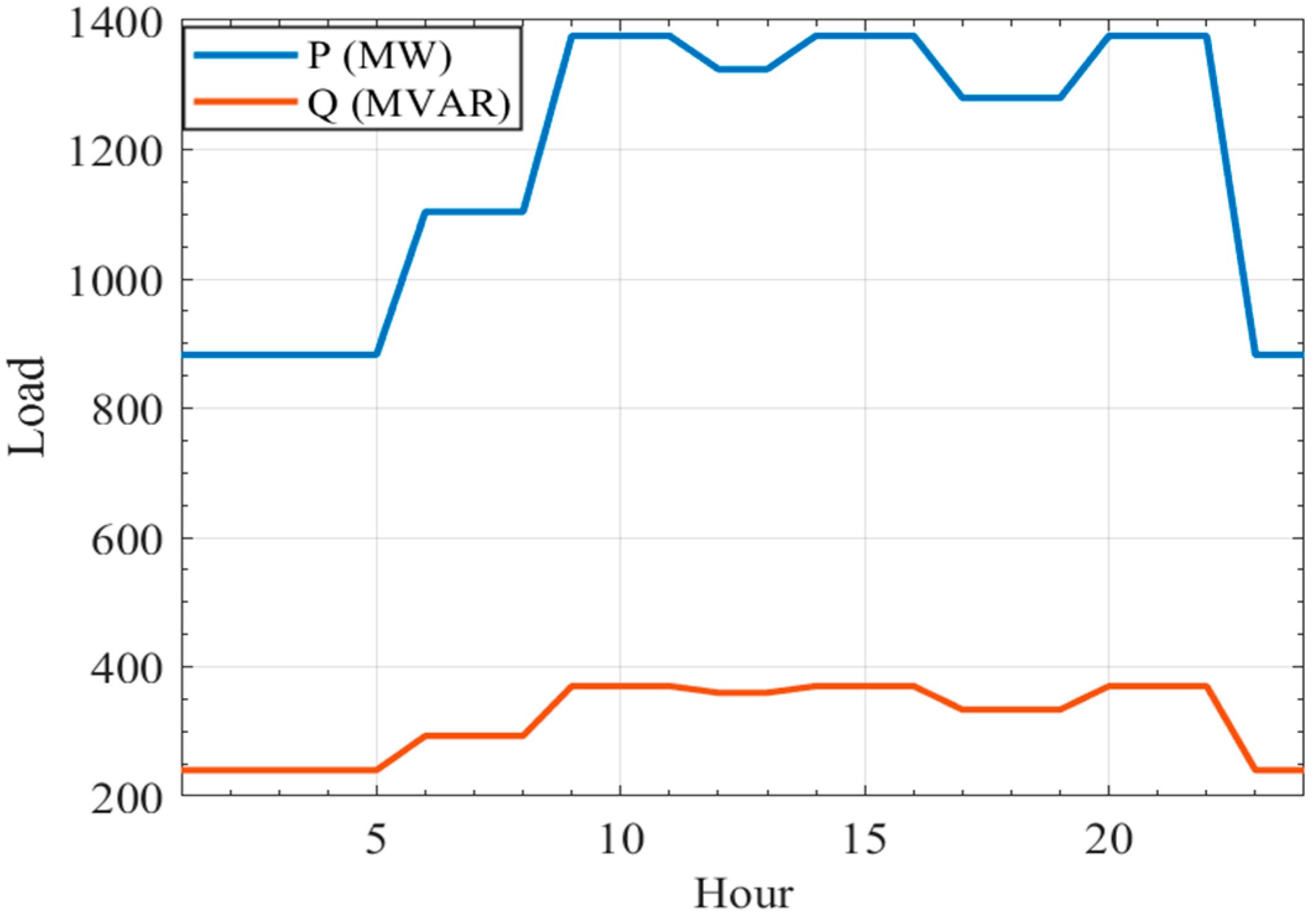
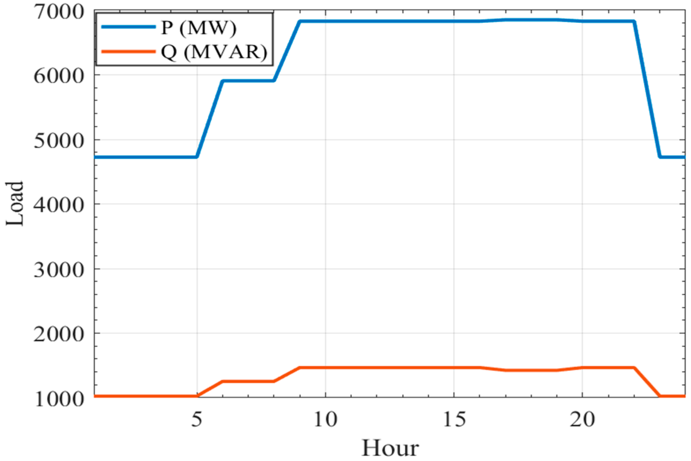
The CSA optimization method is used to perform the POPF. The system used in this subsection is the IEEE 57-bus system, with modifications. The PV and WT generators are inserted into the test system at specified buses. The PV array is connected to bus 37. Meanwhile, the WT farm is connected to bus 12. The loads are assumed to change hourly, as shown in Figure 5 [47]. The one-line diagram of the standard 57-bus test network can be found in Figure A1, in Appendix A. The location of the PV array is marked with red in the single-line diagram, while the location of the wind turbine is marked in green.
The generated power of the RESs changes based on the irradiance, as well as with wind speed [48,49]. Accordingly, the stochastic nature of the RESs [40] should be taken into consideration to properly forecast the generated power from the solar and wind systems. In this subsection, various conditions of POPF are investigated. First, the OPF problem is tested on both test networks, using changing loads. No RESs are inserted into the grids. In the second and third tests, the POPF problem is studied using the 57-bus system, including only one type of RES in the system. In the fourth case, the POPF is tackled by integrating the two kinds of RESs into the 57-bus test system.
The nominal wind speed, allowable cut-in, and cut-off speeds of wind to operate the WT are set to 15, 2.7, and 25 m/s, respectively. The solar irradiance is set to 1000 W/m2 in standard conditions. The certain irradiance point (Rc) is set to 120 W/m
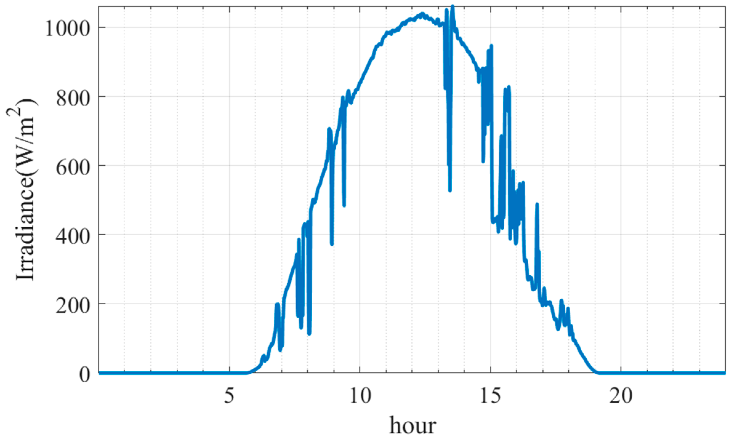
2. This subsection aims to show the effect of integrating the RESs with the uncertain nature of the system and the reflection of this integration on the generation costs of the fuel generators. The installation costs of the RESs are not included in the cost function of this study. The POPF is performed independently at each hour of the day. The measurements of wind speeds used for this study were performed in Zafarana in Egypt on 6 March 2015. The Natural Energy Laboratory of Hawaii Authority (NELHA) provided the solar irradiance measurements on 13 June 2022. The readings of solar irradiance and the wind speeds were plotted, as shown in Figure 6 and Figure 7.
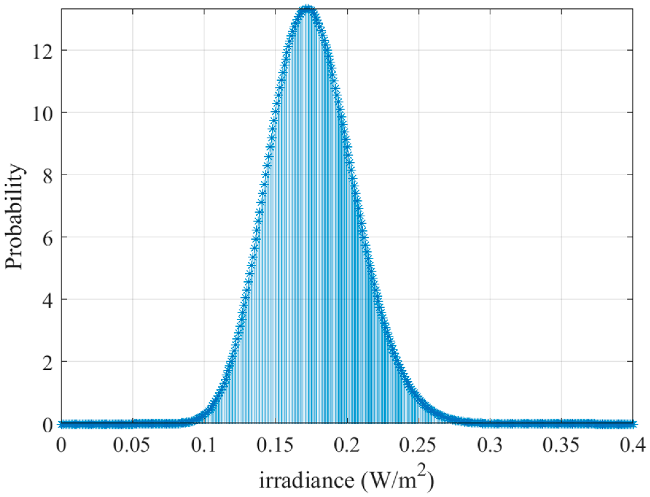
Moreover, the PDFs of the solar irradiance and the wind speed at hour 18 are provided in Figure 8 and Figure 9 as examples of the PDFs of solar irradiance and wind speeds at any hour through the day. The forecasted power generation of the RESs can then be determined, as mathematically shown in Equations (15) and (19).
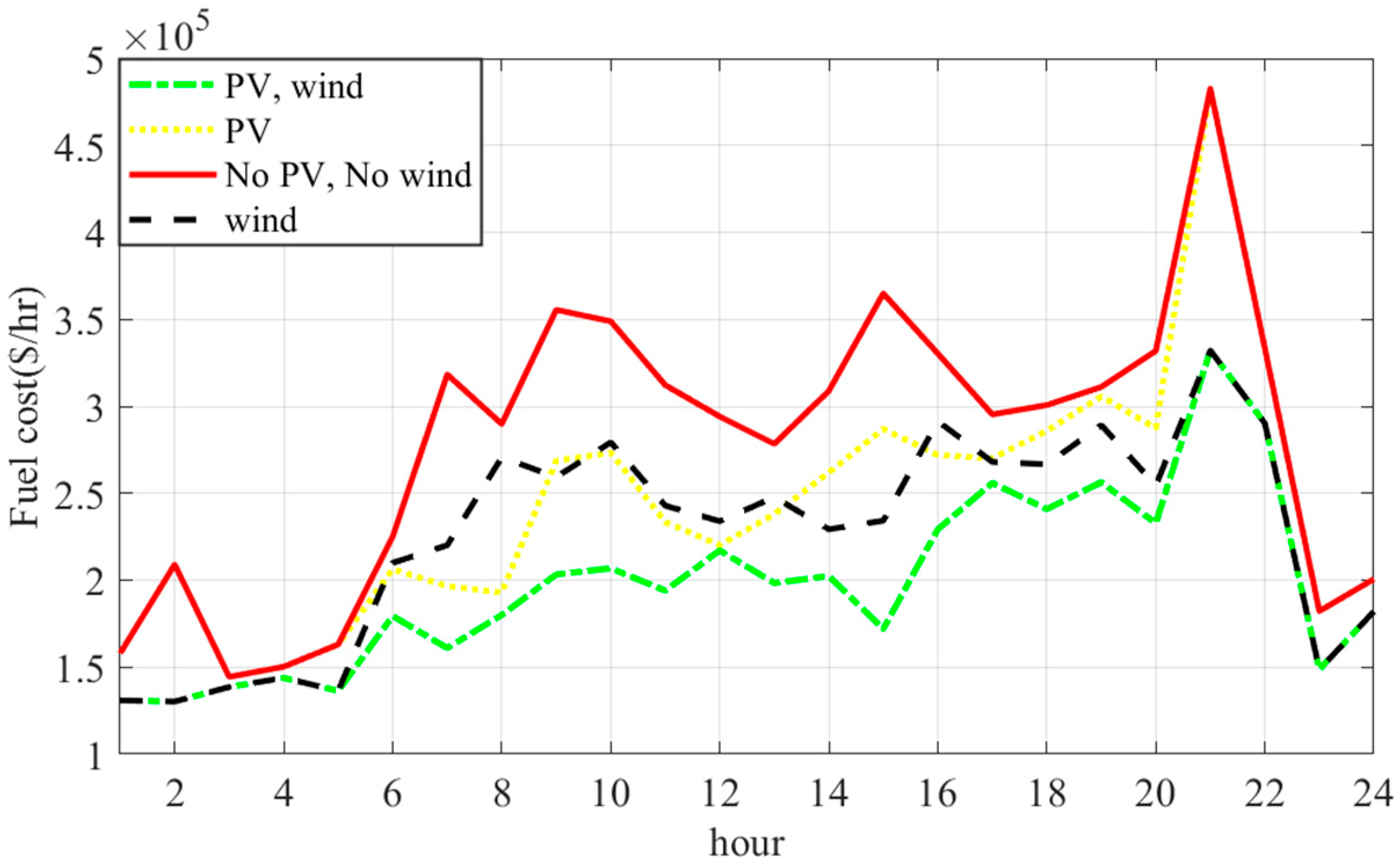
After the simulation is complete and the POPF results are obtained in the four mentioned cases, using the proposed CSA optimization algorithm, the comparisons of the fuel costs of the conventional generators in the four cases can be graphically illustrated, as shown in Figure 10 for the 57-bus test network. The effect of the power generated from the PV systems is observed between hours 6 and 19. This is when solar irradiance is more effective in generating electrical power. The PV cannot be used to generate power beyond this period. On the other hand, the second type of RES connected to the systems, the wind turbine, can generate power at any time, as long as the actual wind speed is within the range of the cut-in and cut-off speeds. The cost reduction due to the integration of the WT can be observed throughout a typical day.

5.1.3. Statistical Investigation of the Classical OPF Results

The statistical analysis aims to investigate how robust the proposed CSA optimization algorithm is when solving the classical OPF optimization problem. The robustness is measured by repeating the simulation 20 times, independently. Repeated runs were also performed with the PSO and the GA. The statistical analysis was performed with the IEEE 57-bus system. The simulation results of the repeated runs of the three optimization methods are observed and compared, as shown in Table 3. Comparing the results verified the robustness of the introduced CSA optimization method.
The final test to be performed was Wilcoxon’s rank-sum test. These test results were compared among the three presented optimization methods. These comparisons are provided in Table 4. The level of significance was set at 5%. It can be seen from the test results that the h-values were equal to ‘1’. The results of Wilcoxon’s rank-sum confirmed the superiority of the proposed CSA optimization method over the PSO algorithm, the GA, and the ML-TSO in optimizing the OPF optimization problem solution.

5.2. Second Test System: The IEEE 118-Bus Test Network

5.2.1. The Classical OPF Results

The same optimization problem was tackled by the GA, ML-TSO, and PSO algorithms to verify the simulation results achieved by the proposed CSA algorithm. The stopping criterion of the compared optimization methods’ simulation process was 600 iterations. The simulation results of the classical model were then compared and the results are shown in Table 5. The design variables are also included in the tables. The design variables are the power generated by conventional generators. Figure 11 provides a more graphical comparison between the convergence performance of the CSA, the GA, the ML-TSO, and the PSO in the IEEE 118-bus test system. In this figure, a focus on the last three iterations is also shown.
It can be seen that the proposed CSA optimization algorithm reached the best solution at the end of the iterations. The CSA needed no more than 200 iterations to gain a better solution, compared to the GA and the PSO algorithms. After 600 iterations, the proposed CSA optimization algorithm achieved better simulation results when solving the classical OPF than the GA by 6.585%. Compared with the PSO algorithm, the proposed CSA optimization algorithm obtained results with a 2.7392% improvement. Compared with the ML-TSO algorithm, the proposed CSA optimization algorithm obtained results with an 0.173% improvement. Generally, the objective in both the studied systems converged rapidly and smoothly.

5.2.2. The POPF with RES Uncertainties and Changing Loads

The loads were assumed to change hourly, as shown in Figure 12 [
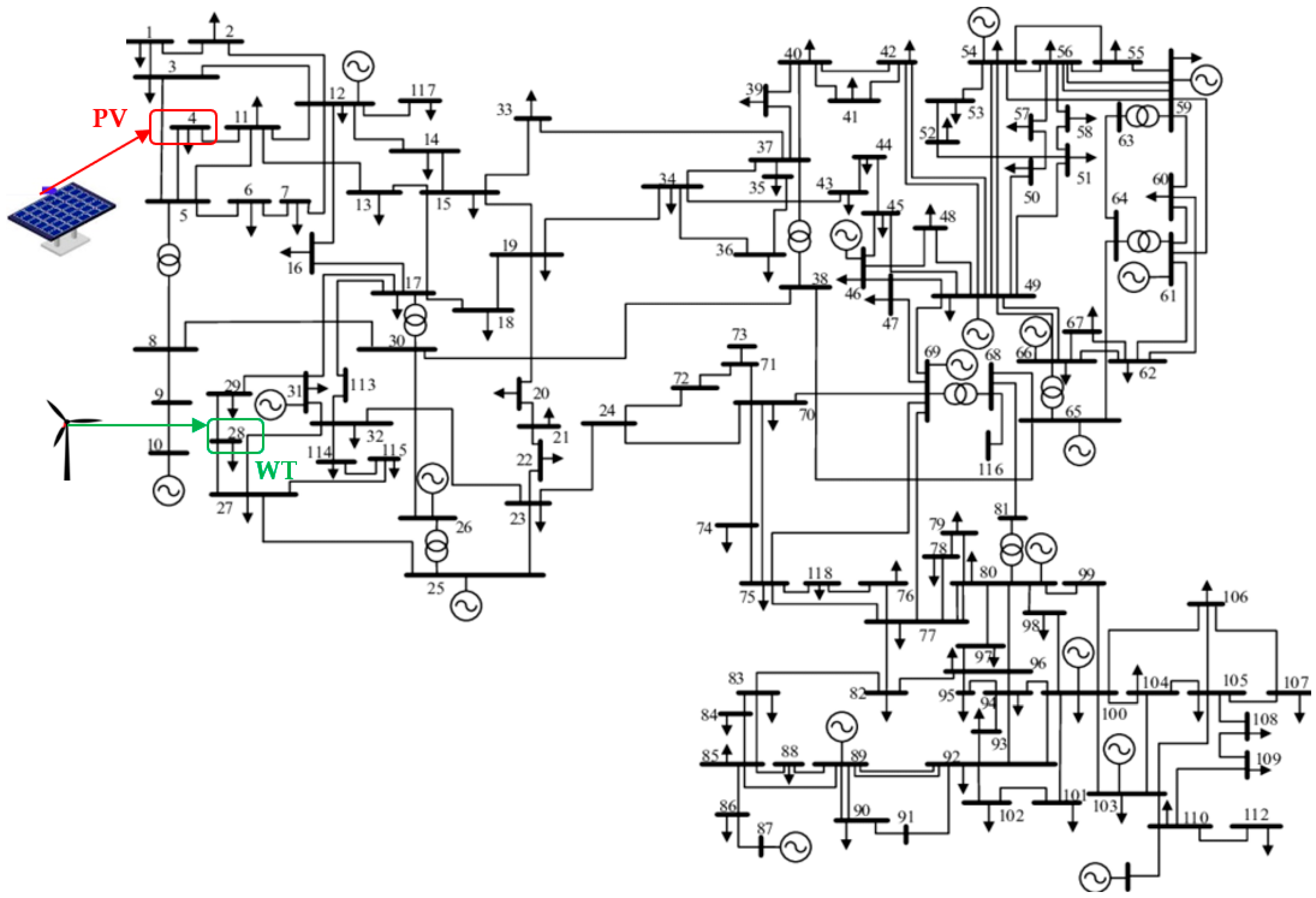
47]. The PV panels were connected to bus 4. Meanwhile, the WT was connected to bus 28. The one-line diagram of the standard IEEE 118-bus system is provided in Figure A2 in the Appendix A. The location of the PV panels is marked in red in the single-line diagram, while the sites of the WT are marked in green.
After the simulation was performed and the POPF results were obtained in the four previously mentioned cases, using the proposed CSA optimization algorithm, the comparisons of the fuel costs of the conventional generators in the four cases were established and are graphically illustrated in Figure 13 for the 118-bus system.

5.2.3. Statistical Investigation of the Classical OPF Results

The robustness of the model was measured by repeating the simulations 20 times, independently. The repeated runs were also performed for the PSO, the GA, and the ML-TSO models. The statistical analysis was performed with the IEEE 118-bus system. The simulation results of the repeated runs of the three optimization methods were observed and compared and are shown in Table 6. Comparing the results verified the robustness of the introduced CSA optimization method.
Wilcoxon’s rank-sum test results were compared among the three presented optimization methods. These comparisons are provided in Table 7. The level of significance is set to 5%. It can be observed from the test results that the h-values are equal to ‘1’. The results of Wilcoxon’s rank-sum test confirmed the superiority of the proposed CSA optimization method over the PSO algorithm, the GA, and the ML-TSO in optimizing the OPF optimization problem solution.

6. Conclusions

This paper presents a novel CSA optimization algorithm to address power system optimization problems, specifically, the OPF and POPF problems. The CSA technique was tested on the IEEE 57-bus test system and the IEEE 118-bus test system. The simulation results and comparison with other well-known algorithms, GA and PSO, as well as the metaheuristic, recently published algorithm, ML-TSO, confirmed the superiority and robustness of the developed CSA technique. Using the proposed CSA to solve the OPF problem led to a generation cost reduction from 0.044079% to 0.9306%, validated on a 57-bus system, and by 0.173% to 6.585% when testing on the 118-bus system. Furthermore, the development of CSA enabled us to solve the POPF problem, addressing the intermittent nature of the RESs and load variation throughout the day using distribution functions. According to the simulation results, the generation costs have been sufficiently reduced due to the insertion of the RESs into both test systems. Statistical analysis in comparison with other algorithms is also provided to discuss the results further and to support the evaluation of the proposed optimization algorithm. For future work, it is recommended that researchers should apply the CSA optimization algorithm to other optimization problems within the scope of renewable energy systems.

Author Contributions

H.M.H.: Formal analysis, investigation of the results, methodology, supervision, validation of the results, review and editing of the article; M.H.Q., Z.U., M.T.-V., R.A.T., F.J., M.R.E., M.A.M.S., K.J.C.: Software modification, simulation, writing, and editing. All authors have read and agreed to the published version of the manuscript.

Funding

This research has no funding.

Data Availability Statement

Not applicable.

Conflicts of Interest

The authors declare no conflict of interest.

Appendix A

Figure A1. Single-line diagram of the IEEE 57-bus system.
Energies 15 08303 g0a1
Figure A2. Single-line diagram of the IEEE 118-bus system.
Energies 15 08303 g0a2

References

  1. Lee, J.-O.; Kim, Y.-S.; Jeon, J.-H. Optimal power flow for bipolar DC microgrids. Int. J. Electr. Power Energy Syst. 2022, 142, 108375. [Google Scholar] [CrossRef]
  2. González-Cabrera, N.; Castro, L.M.; Gutiérrez-Alcaraz, G.; Tovar-Hernandez, J. Alternative approach for efficient OPF calculations in hybrid AC/DC power grids with VSC-HVDC systems based on shift factors. Int. J. Electr. Power Energy Syst. 2021, 124, 106395. [Google Scholar] [CrossRef]
  3. Dash, S.P.; Subhashini, K.; Chinta, P. Development of a boundary assigned animal migration optimization algorithm and its application to optimal power flow study. Expert Syst. Appl. 2022, 200, 116776. [Google Scholar] [CrossRef]
  4. Shaheen, A.M.; El-Sehiemy, R.A.; Hasanien, H.M.; Ginidi, A.R. An improved heap optimization algorithm for efficient energy management based optimal power flow model. Energy 2022, 250, 123795. [Google Scholar] [CrossRef]
  5. Thukaram, B.D.; Parthasarathy, K. Optimal reactive power dispatch algorithm for voltage stability improvement. Int. J. Electr. Power Energy Syst. 1996, 18, 461–468. [Google Scholar] [CrossRef]
  6. Xie, K.; Liu, M.; Lu, W.; Wu, J. Discrete/continuous-time online algorithm application for time-varying optimal power flow in active distribution networks. Int. J. Electr. Power Energy Syst. 2022, 138, 107859. [Google Scholar] [CrossRef]
  7. Kahraman, H.T.; Akbel, M.; Duman, S. Optimization of optimal power flow problem using multi-objective manta ray foraging optimizer. Appl. Soft Comput. 2022, 116, 108334. [Google Scholar] [CrossRef]
  8. Montoya, O.D. A convex OPF approximation for selecting the best candidate nodes for optimal location of power sources on DC resistive networks. Eng. Sci. Technol. Int. J. 2020, 23, 527–533. [Google Scholar] [CrossRef]
  9. Zhang, J.; Zhu, X.; Li, P. MOEA/D with many-stage dynamical resource allocation strategy to solution of many-objective OPF problems. Int. J. Electr. Power Energy Syst. 2020, 120, 106050. [Google Scholar] [CrossRef]
  10. Li, Q.; Zhao, N. A probability box representation method for power flow analysis considering both interval and probabilistic uncertainties. Int. J. Electr. Power Energy Syst. 2022, 142, 108371. [Google Scholar] [CrossRef]
  11. Dumas, J.; Wehenkel, A.; Lanaspeze, D.; Cornélusse, B.; Sutera, A. A deep generative model for probabilistic energy forecasting in power systems: Normalizing flows. Appl. Energy 2021, 305, 117871. [Google Scholar] [CrossRef]
  12. Rajamand, S. Probabilistic power distribution considering uncertainty in load and distributed generators using cumulant and truncated versatile distribution. Sustain. Energy Grids Netw. 2022, 30, 100608. [Google Scholar] [CrossRef]
  13. Rouhani, M.; Mohammadi, M.; Aiello, M. Soft clustering based probabilistic power flow with correlated inter temporal events. Electr. Power Syst. Res. 2022, 204, 107677. [Google Scholar] [CrossRef]
  14. Alzubaidi, M.; Hasan, K.N.; Meegahapola, L. Impact of probabilistic modelling of wind speed on power system voltage profile and voltage stability analysis. Electr. Power Syst. Res. 2022, 206, 107807. [Google Scholar] [CrossRef]
  15. Lotfi, M.; Osório, G.J.; Javadi, M.S.; El Moursi, M.S.; Monteiro, C.; Catalão, J.P. A fully decentralized machine learning algorithm for optimal power flow with cooperative information exchange. Int. J. Electr. Power Energy Syst. 2022, 139, 107990. [Google Scholar] [CrossRef]
  16. Shaheen, M.A.M.; Hasanien, H.M.; Mekhamer, S.F.; Qais, M.H.; Alghuwainem, S.; Ullah, Z.; Tostado-Véliz, M.; Turky, R.A.; Jurado, F.; Elkadeem, M.R. Probabilistic optimal power flow solution using a novel hybrid metaheuristic and machine learning algorithm. Mathematics 2022, 10, 3036. [Google Scholar] [CrossRef]
  17. Wang, M.; Yin, Y.; Yang, M.; Han, X. Probabilistic power flow calculation considering electro-thermo-mechanical dynamics of overhead conductor. Int. J. Electr. Power Energy Syst. 2022, 143, 108374. [Google Scholar] [CrossRef]
  18. Riaz, M.; Hashmi, M.R. Linear Diophantine fuzzy set and its applications towards multi-attribute decision-making problems. J. Intell. Fuzzy Syst. 2019, 37, 5417–5439. [Google Scholar] [CrossRef]
  19. Riaz, M.; Sałabun, W.; Farid, H.M.A.; Ali, N.; Wątróbski, J. A Robust q-rung Orthopair fuzzy information aggregation using einstein operations with application to sustainable energy planning decision management. Energies 2020, 13, 2155. [Google Scholar] [CrossRef]
  20. Lin, X.; Shu, T.; Tang, J.; Ponci, F.; Monti, A.; Li, W. Application of joint raw moments-based probabilistic power flow analysis for hybrid AC/VSC-MTDC power systems. IEEE Trans. Power Syst. 2022, 37, 1399–1412. [Google Scholar] [CrossRef]
  21. Sun, Y.; Xia, D.; Gao, Z.; Wang, Z.; Li, G.; Lu, W.; Wu, X.; Li, Y. Probabilistic load flow calculation of AC/DC hybrid system based on cumulant method. Int. J. Electr. Power Energy Syst. 2022, 139, 107998. [Google Scholar] [CrossRef]
  22. Lin, C.; Bie, Z.; Pan, C.; Liu, S. Fast cumulant method for probabilistic power flow considering the nonlinear relationship of wind power generation. IEEE Trans. Power Syst. 2020, 35, 2537–2548. [Google Scholar] [CrossRef]
  23. Sheng, H.; Wang, X. Probabilistic power flow calculation using non-intrusive low-rank approximation method. IEEE Trans. Power Syst. 2019, 34, 3014–3025. [Google Scholar] [CrossRef] [Green Version]
  24. Xie, Z.Q.; Ji, T.Y.; Li, M.S.; Wu, Q.H. Quasi-monte carlo based probabilistic optimal power flow considering the correlation of wind speeds using copula function. IEEE Trans. Power Syst. 2018, 33, 2239–2247. [Google Scholar] [CrossRef]
  25. Zuluaga, C.D.; Alvarez, M.A. Bayesian Probabilistic power flow analysis using Jacobian approximate Bayesian computation. IEEE Trans. Power Syst. 2018, 33, 5217–5225. [Google Scholar] [CrossRef]
  26. Sun, W.; Zamani, M.; Zhang, H.-T.; Li, Y. Probabilistic optimal power flow with correlated wind power uncertainty via markov chain Quasi-Monte-Carlo sampling. IEEE Trans. Ind. Inform. 2019, 15, 6058–6069. [Google Scholar] [CrossRef]
  27. Li, Q.; Zhao, N. Probabilistic power flow calculation based on importance-Hammersley sampling with Eigen-decomposition. Int. J. Electr. Power Energy Syst. 2021, 130, 106947. [Google Scholar] [CrossRef]
  28. Lin, X.; Jiang, Y.; Peng, S.; Chen, H.; Tang, J.; Li, W. An efficient Nataf transformation based probabilistic power flow for high-dimensional correlated uncertainty sources in operation. Int. J. Electr. Power Energy Syst. 2020, 116, 105543. [Google Scholar] [CrossRef]
  29. Uniyal, A.; Sarangi, S. Optimal network reconfiguration and DG allocation using adaptive modified whale optimization algorithm considering probabilistic load flow. Electr. Power Syst. Res. 2020, 192, 106909. [Google Scholar] [CrossRef]
  30. Qais, M.H.; Hasanien, H.M.; Turky, R.A.; Alghuwainem, S.; Tostado-Véliz, M.; Jurado, F. Circle search algorithm: A geometry-based metaheuristic optimization algorithm. Mathematics 2022, 10, 1626. [Google Scholar] [CrossRef]
  31. Karmouni, H.; Chouiekh, M.; Motahhir, S.; Qjidaa, H.; Jamil, M.O.; Sayyouri, M. Optimization and implementation of a photovoltaic pumping system using the sine–cosine algorithm. Eng. Appl. Artif. Intell. 2022, 114, 105104. [Google Scholar] [CrossRef]
  32. Elaziz, M.A.; Ewees, A.A.; Al-Qaness, M.A.; Abualigah, L.; Ibrahim, R.A. Sine-Cosine-Barnacles algorithm optimizer with disruption operator for global optimization and automatic data clustering. Expert Syst. Appl. 2022, 207, 117993. [Google Scholar] [CrossRef]
  33. Shaheen, M.A.M.; Hasanien, H.M.; Mekhamer, S.F.; Talaat, H.E.A. Optimal power flow of power networks with penetration of renewable energy sources by Harris hawks optimization method. In Proceedings of the 2020 2nd International Conference on Smart Power and Internet Energy Systems (SPIES), Bangkok, Thailand, 15–18 September 2020. [Google Scholar] [CrossRef]
  34. Shaheen, M.A.M.; Hasanien, H.M.; Al-Durra, A. Solving of optimal power flow problem including renewable energy resources using heap optimization algorithm. IEEE Access 2021, 9, 35846–35863. [Google Scholar] [CrossRef]
  35. Shaheen, M.; Mekhamer, S.F.; Hasanien, H.M.; Talaat, H.E.A. Optimal power flow of power systems using hybrid firefly and particle swarm optimization technique. In Proceedings of the 2019 21st International Middle East Power Systems Conference (MEPCON), Cairo, Egypt, 17–19 December 2019. [Google Scholar]
  36. Shaheen, M.A.M.; Hasanien, H.M.; Mekhamer, S.F.; Talaat, H.E.A. Optimal Power Flow of Power Systems Including Distributed Generation Units Using Sunflower Optimization Algorithm. IEEE Access 2019, 7, 109289–109300. [Google Scholar] [CrossRef]
  37. Ramírez, A.F.; Valencia, C.F.; Cabrales, S.; Ramírez, C.G. Simulation of photo-voltaic power generation using copula autoregressive models for solar irradiance and air temperature time series. Renew. Energy 2021, 175, 44–67. [Google Scholar] [CrossRef]
  38. Scarabaggio, P.; Grammatico, S.; Carli, R.; Dotoli, M. Distributed demand side management with stochastic wind power forecasting. IEEE Trans. Control Syst. Technol. 2021, 30, 97–112. [Google Scholar] [CrossRef]
  39. Khosravi, M.; Afsharnia, S.; Farhangi, S. Stochastic power management strategy for optimal day-ahead scheduling of wind-HESS considering wind power generation and market price uncertainties. Int. J. Electr. Power Energy Syst. 2022, 134, 107429. [Google Scholar] [CrossRef]
  40. Kaymaz, E.; Duman, S.; Guvenc, U. Optimal power flow solution with stochastic wind power using the Lévy coyote optimization algorithm. Neural Comput. Appl. 2021, 33, 6775–6804. [Google Scholar] [CrossRef]
  41. Sun, L.; You, F. Machine learning and data-driven techniques for the control of smart power generation systems: An uncertainty handling perspective. Engineering 2021, 7, 1239–1247. [Google Scholar] [CrossRef]
  42. Luo, Y.; Wang, Z.; Zhu, J.; Lu, T.; Xiao, G.; Chu, F.; Wang, R. Multi-objective robust optimization of a solar power tower plant under uncertainty. Energy 2022, 238, 121716. [Google Scholar] [CrossRef]
  43. He, Y.; Li, H.; Wang, S.; Yao, X. Uncertainty analysis of wind power probability density forecasting based on cubic spline interpolation and support vector quantile regression. Neurocomputing 2021, 430, 121–137. [Google Scholar] [CrossRef]
  44. Zeng, L.; Xu, J.; Wu, M.; Tang, J.; Wu, Q.; Wang, Q.; Fan, G. Day-ahead interval optimization for CCHP system considering uncertainty of wind power and PV. Int. J. Electr. Power Energy Syst. 2022, 138, 107895. [Google Scholar] [CrossRef]
  45. Ullah, Z.; Wang, S.; Radosavljevic, J.; Lai, J. A solution to the optimal power flow problem considering WT and PV generation. IEEE Access 2019, 7, 46763–46772. [Google Scholar] [CrossRef]
  46. Chegini, S.N.; Bagheri, A.; Najafi, F. PSOSCALF: A new hybrid PSO based on sine cosine algorithm and levy flight for solving optimization problems. Appl. Soft Comput. 2018, 73, 697–726. [Google Scholar] [CrossRef]
  47. Cuevas, E.; Galvez, J. An optimization algorithm guided by a machine learning approach. Int. J. Mach. Learn. Cybern. 2019, 10, 2963–2991. [Google Scholar] [CrossRef]
  48. Li, S.; Gong, W.; Wang, L.; Gu, Q. Multi-objective optimal power flow with stochastic wind and solar power. Appl. Soft Comput. 2022, 114, 108045. [Google Scholar] [CrossRef]
  49. Aliabadi, M.J.; Radmehr, M. Optimization of hybrid renewable energy system in radial distribution networks considering uncertainty using meta-heuristic crow search algorithm. Appl. Soft Comput. 2021, 107, 107384. [Google Scholar] [CrossRef]
Figure 1. The decrease in the angle for exploitation in the CSA.
Energies 15 08303 g001
Figure 2. The exploration in the CSA.
Energies 15 08303 g002
Figure 3. The steps of problem-solving using the CSA.
Energies 15 08303 g003
Figure 4. Convergence performance of the CSA, the GA, and the PSO in the case of the 57-bus system.
Energies 15 08303 g004
Figure 5. Variations in P and Q in the 57-bus test network.
Energies 15 08303 g005
Figure 6. Wind speeds through a typical day.
Energies 15 08303 g006
Figure 7. Solar irradiance through a typical day.
Energies 15 08303 g007
Figure 8. Probability density function of solar irradiance at hour 18.
Energies 15 08303 g008
Figure 9. Probability density function of wind speed at hour 18.
Energies 15 08303 g009
Figure 10. Cost variations of the 57-bus test network.
Energies 15 08303 g010
Figure 11. Convergence performance of the CSA, the GA, and the PSO in the case of the 118-bus system.
Energies 15 08303 g011
Figure 12. Variations in the P and Q of the IEEE 118-bus system.
Energies 15 08303 g012
Figure 13. Cost variations of the 118-bus test network.
Energies 15 08303 g013
Table 1. The significant specifications of the studied systems.
Studied System57-Bus System [47]118-Bus System [47]
Number of Buses57118
Number of Generations754
Number of Branches80186
Number of Transformers179
Connected loads in MVA1250.0 + j 336.44242 + j 1438
Plosses in MVA16.00 + j 72.97132.86 + j 783.79
Table 2. Minimum objective and optimal design variables in the case of the 57-bus system.
Pgen (MW) at Bus No.CSAGA [47]ML-TSO [16]PSO [47]
1144.6298487151.43944144.8275153.41
293.4229851185.6551593.204340
345.1468779847.3166245.2192147.07
668.5574462763.8144168.2065961.09
8456.659418471.1291456.9922550
995.6306521875.2683295.8449789.58
12366.1451562375.58131365.9111374.31
Simulation time (s)112.86673.58133.28142.92
Minimum cost (USD/h)41,872.9169541,891.374241,872.942,262.61
Table 3. The CSA, GA, and PSO statistical analysis results for the 57-bus test network.
Optimization AlgorithmMin.Max.MeanMedianStd. Dev.
CSA41,872.941,873.241,873.0241,873.0040.076665636
PSO42 × 10342,404.442,133.5442,172.2162.012
GA41,891.442,037.441,938.6241,932.741.01491
ML-TSO41,872.941,872.941,872.941,872.90.00203
Table 4. Wilcoxon’s rank-sum test for the 57-bus test network.
Opt. Algorithm/TestCSA vs. PSOCSA vs. GACSA vs. ML-TSO
p-value (Wilcoxon test)8.8575 × 10−58.8575 × 10−58.8575 × 10⁻⁵
Table 5. Min. objective and optimal design variables in the case of the 118-bus system.
Pgen (MW) at Bus No.CSAGA [47]ML-TSO [16]PSO [47]
15.22295558442.8084325.9724469.35736
46.34031092940.4672619.2893853.66406
623.2074745955.639892.39 × 10−2562.17215
81.88901 × 10−843.7552832.9850348.57892
10420.0099369263.00824383.221810
1278.1793708573.4612584.5644991.82476
153.79901 × 10−1171.500871.48 × 10−10654.09869
185.44755070840.507255.59 × 10−73100
1913.5754643330.798490.0000008930
240.14876261251.1029811.70
25187.026271156.85387185.51225214.13416
26274.4122218136.87232267.134530
2715.7850379739.6330122.5696828.14707
317.65788656633.533743.24 × 10−97.45759
326.98973227635.6798829.4688100
347.35628147248.3699141.13763100
360.00299134542.598726.715160
4032.418368232.4332442.771141.61653
4249.916202834.4289349.50048100
4617.5667183533.1938919.2208919.08021
49201.4539222143.29835190.13596192.63884
5447.4037513164.8675349.895540
5525.5952130140.8934946.573722.03011
5619.9990241556.9588439.51742100
59146.8280053112.15389148.63024149.57239
61146.2882516104.61467144.33423148.24394
622.64462425345.708040.0000002310
65353.3483046243.956903344.15355352.49011
66357.4056727238.35467341.4189349.52639
69452.2006709241.92158441.76801451.7022
7036.5665444161.232321.15 × 10−170
7237.1314819342.5396626.79066100
7311.6235749136.7601632.555180
7425.2903859736.591762.83 × 10−260
763.45394970746.359491.75 × 10−650
770.00097304458.620854.33 × 10−180
80428.947876232.95281426.39416431.30982
850.02203030430.9751700
873.96191950419.631585.401920
89499.6523936385.11713492.9325491.72528
908.04573 × 10−760.1034311.141570.48624
916.24685 × 10−1154.584810.000000240
921.19861 × 10−541.331892.24 × 10−350
990.05282976864.4085718.992360.15028
100226.524279136.28236234.616704226.41352
10333.410012658.1850942.1604937.66295
10416.7154709541.523871.21 × 10−23100
10520.8239935641.387752.59 × 10−90
1070.00030782752.220791.05 × 10−5813.81565
1106.60302097935.336215.626580
11128.9756090248.4283140.1038936.33637
11235.1127150446.518781.2 × 10−230
11317.7338165335.751264.83 × 10−6023.31851
1160.06752976544.7148800
Simulation time (s)223.66776.04272.3270796290.02
Min. cost (USD/h)130,404.016138,991.2993130,630.3451133,976.07655089
Table 6. The CSA, GA, and PSO statistical analysis results for the 118-bus system.
Opt. AlgorithmMin.Max.MeanMedianStd. Dev.
CSA130,404.02132,765.11130,741.43130,529.99577.1176976
PSO132 × 103136 × 103133 × 103133 × 1031140
GA136 × 103140 × 103139 × 103139 × 103856
ML-TSO130,630.34131,124.3130,808.7130,747.18672.0761
Table 7. Wilcoxon’s rank-sum test for the 118-bus test network.
Optimization Method/TestCSA vs. PSOCSA vs. GACSA vs. ML-TSO
p-value (Wilcoxon test)8.8575 × 10−58.8575 × 10−58.8575 × 10⁻⁵
Publisher’s Note: MDPI stays neutral with regard to jurisdictional claims in published maps and institutional affiliations.

