

Toward the Application of Pulse Width Modulated (PWM) Inverter Drive-Based Electric Propulsion to Ice Capable Ships

Abstract
:1. Introduction
2. Problem Description
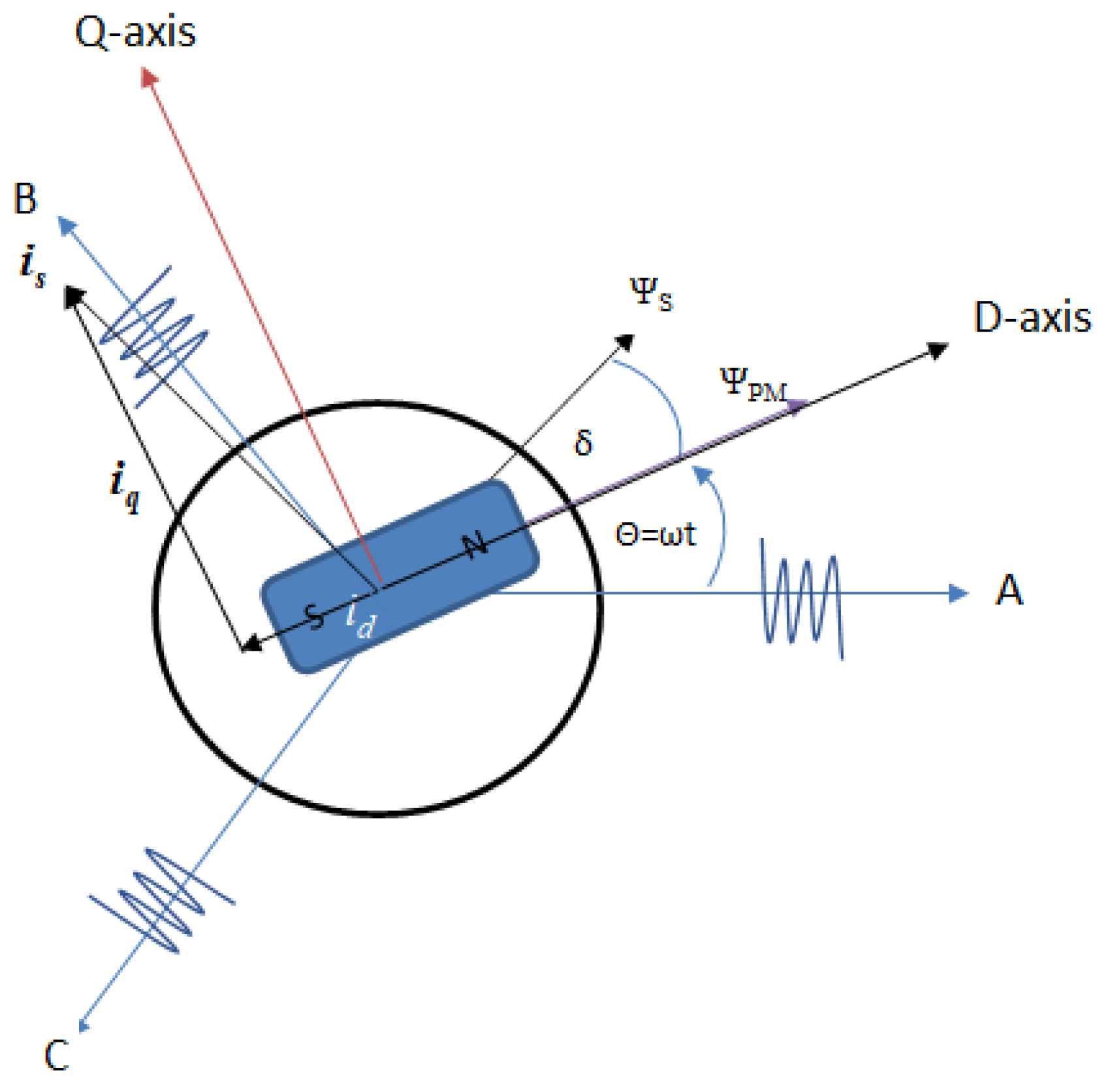
2.1. The Magnetic Flux Space Vector [2]
2.2. The D-Q Reference Frame [2]
2.3. Voltage and Flux Linkage Equations [4]
2.4. PMSM Model Parameters
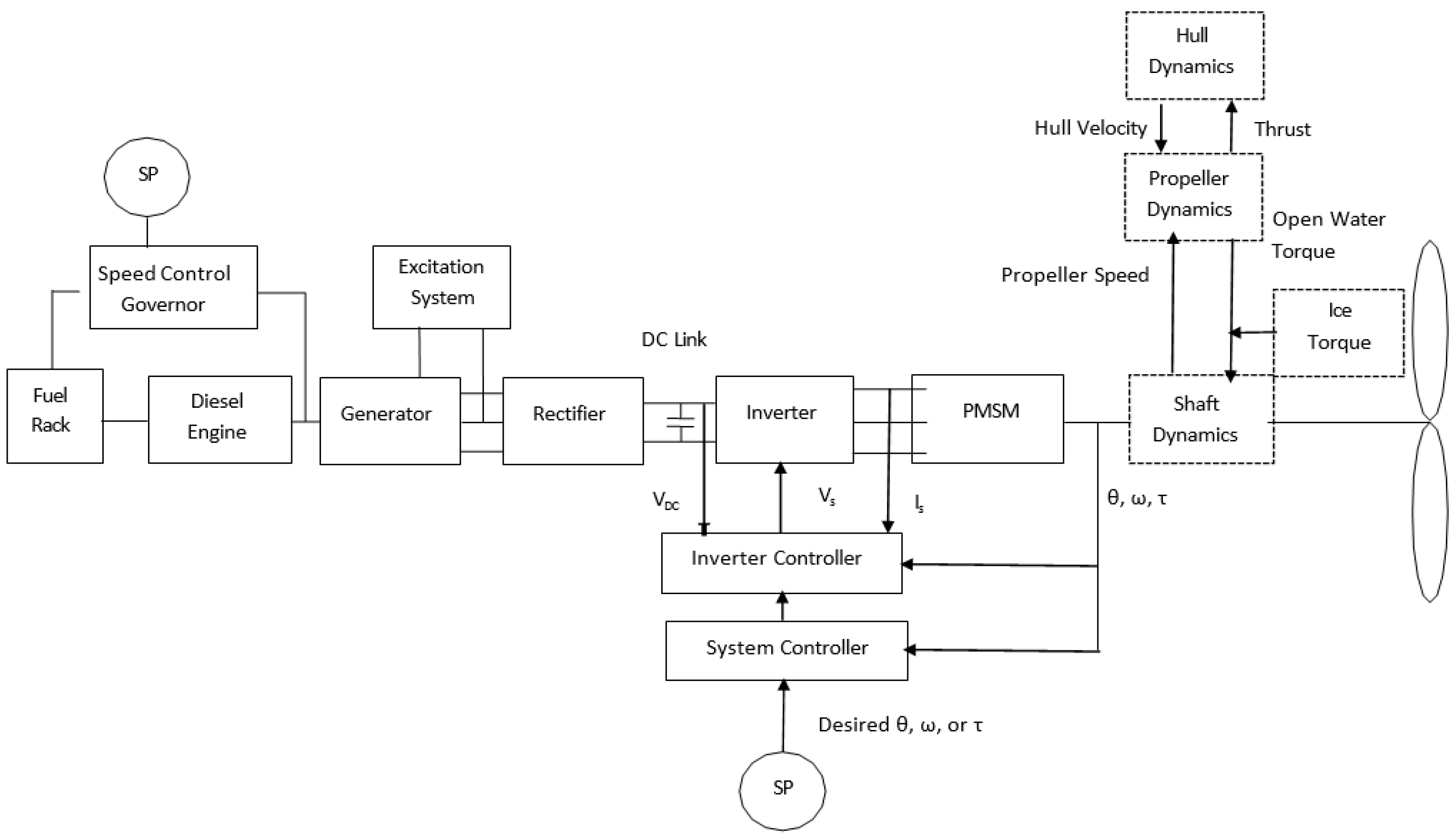
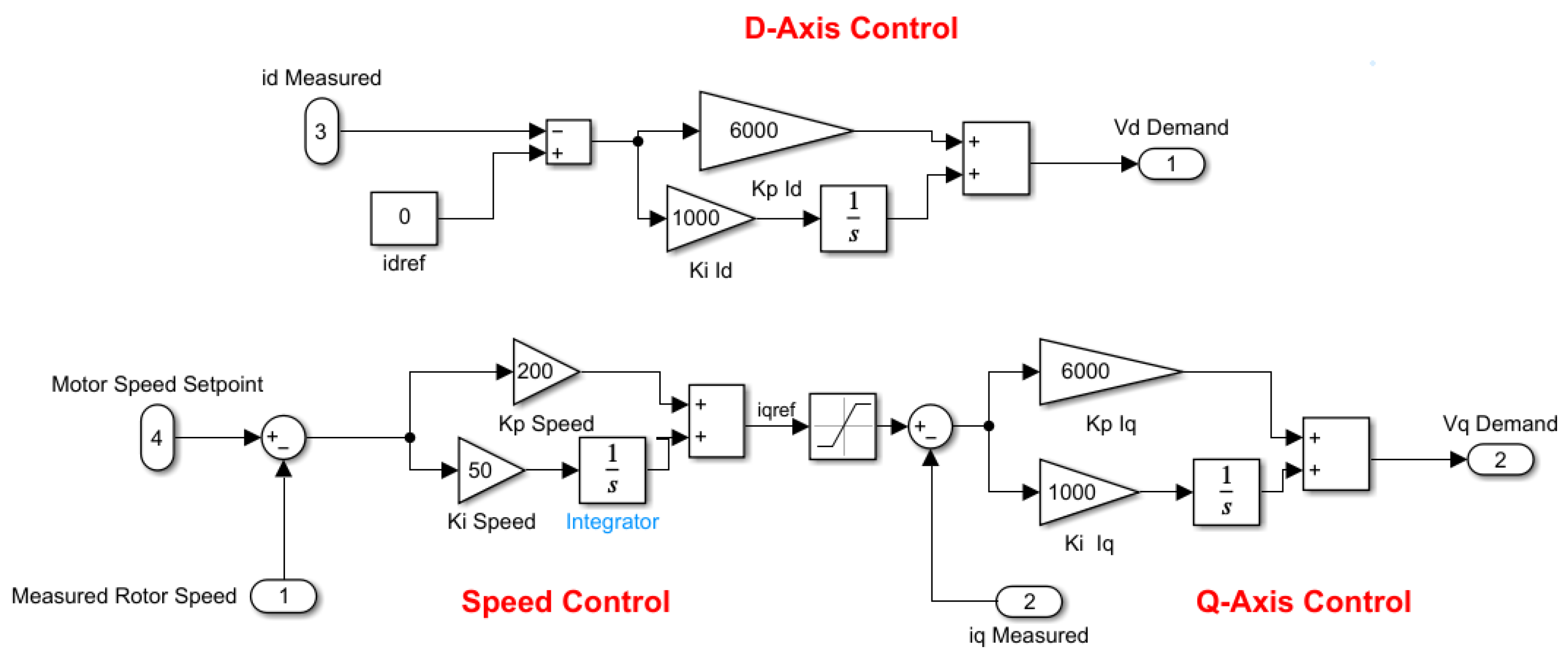
2.5. Motor Control System Overview
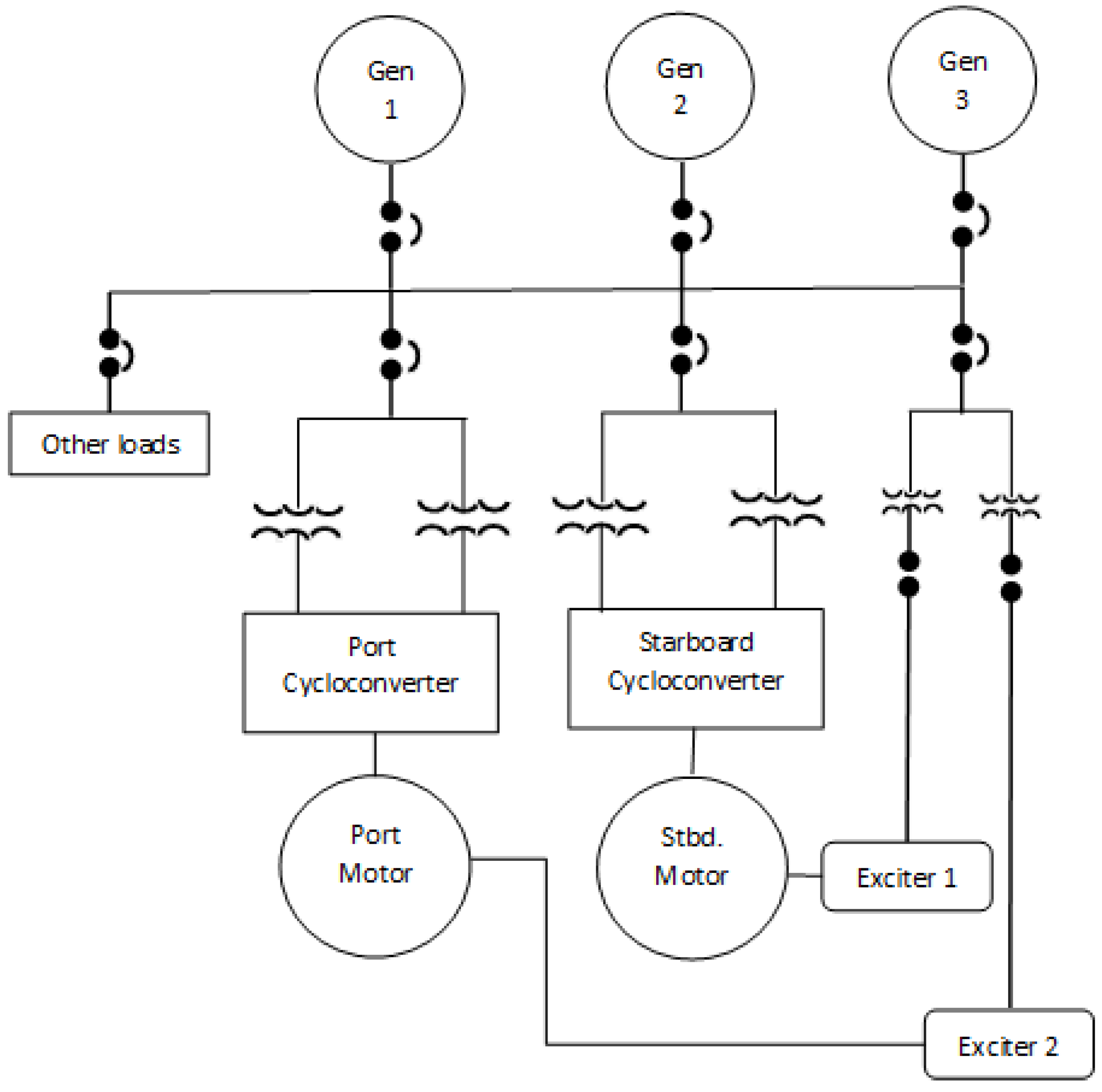
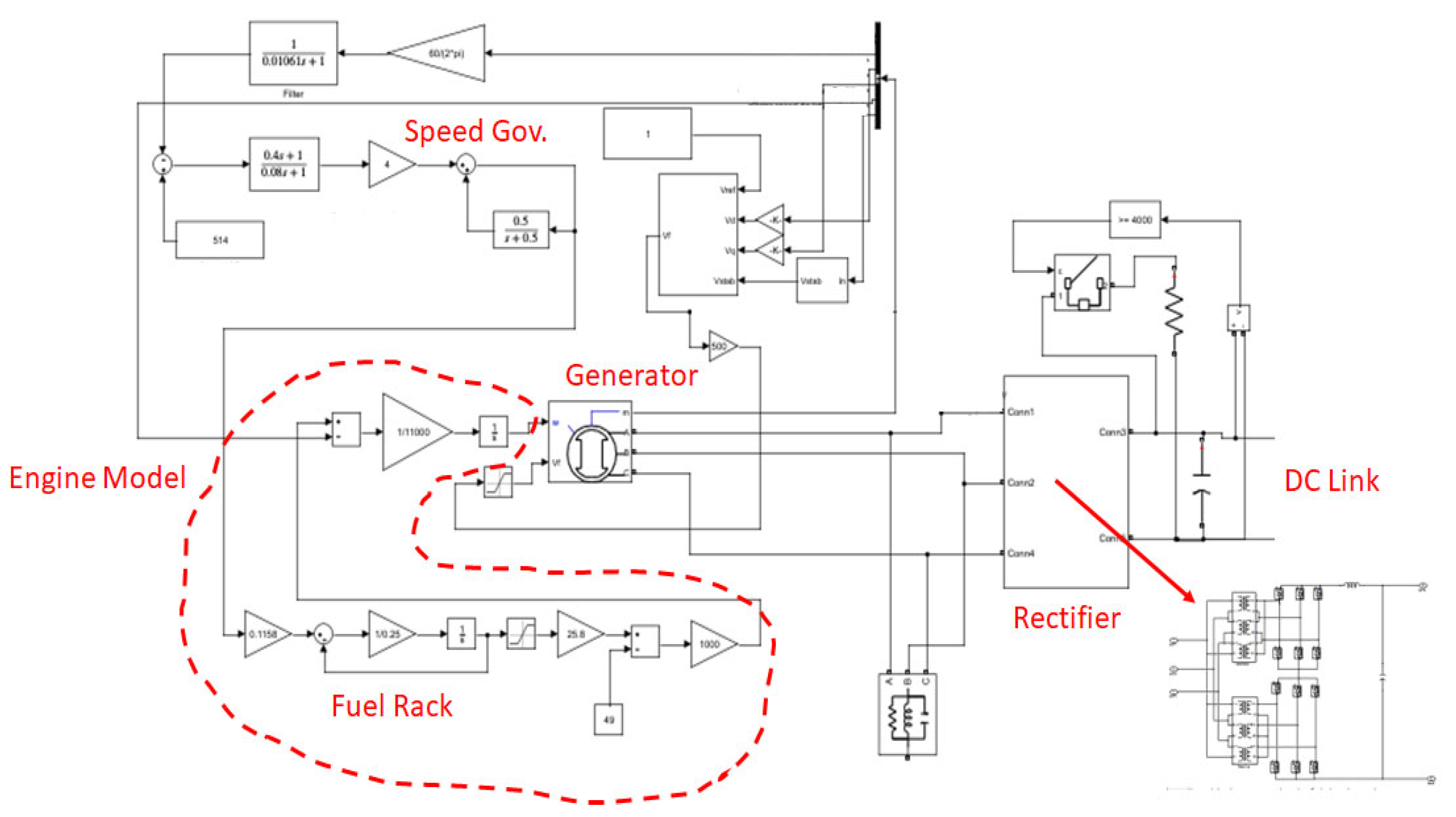
2.6. USCGC Healy Simulink Model
2.7. Engine/Generator
2.8. Rectifier Circuit & DC Link/Filter
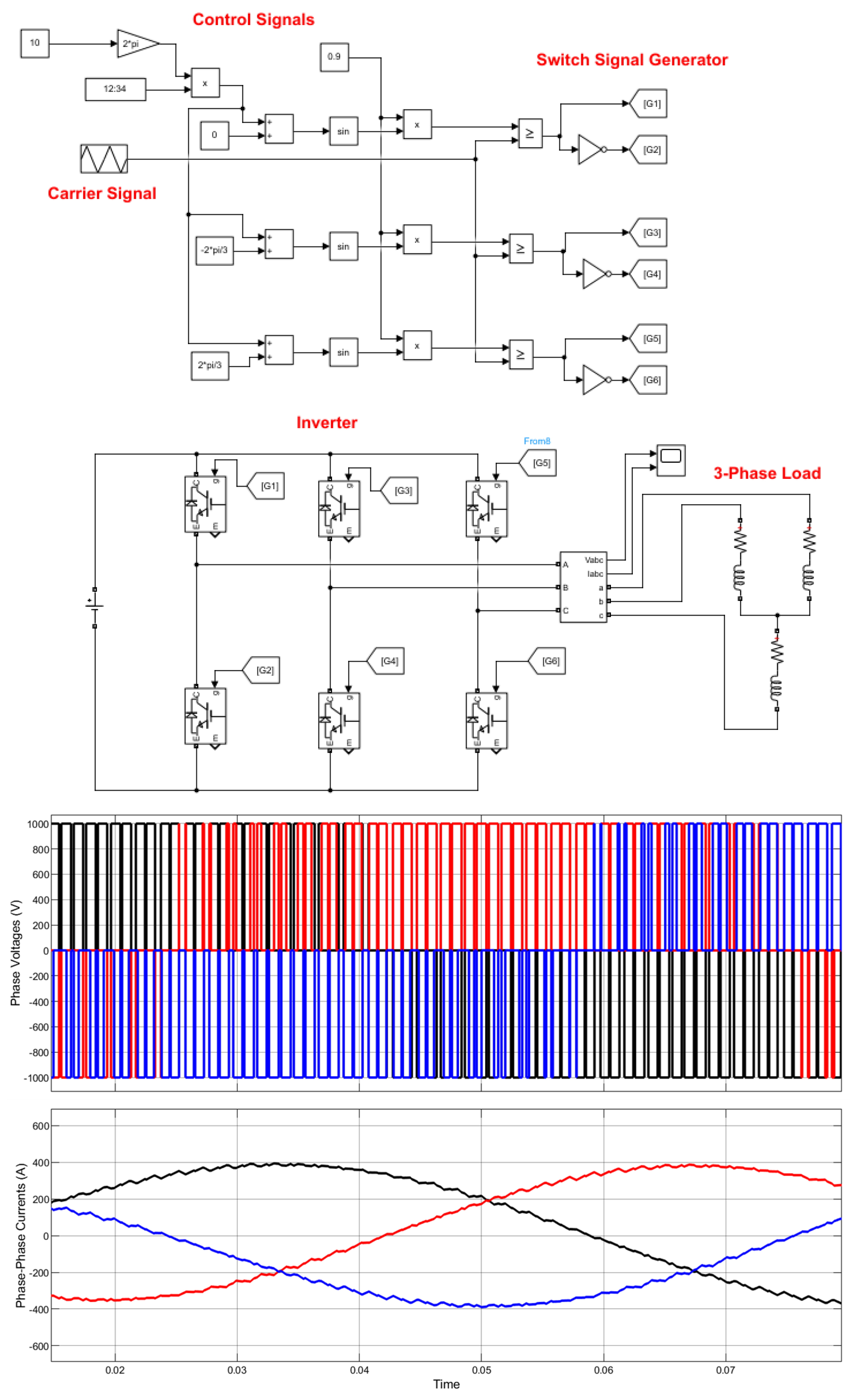
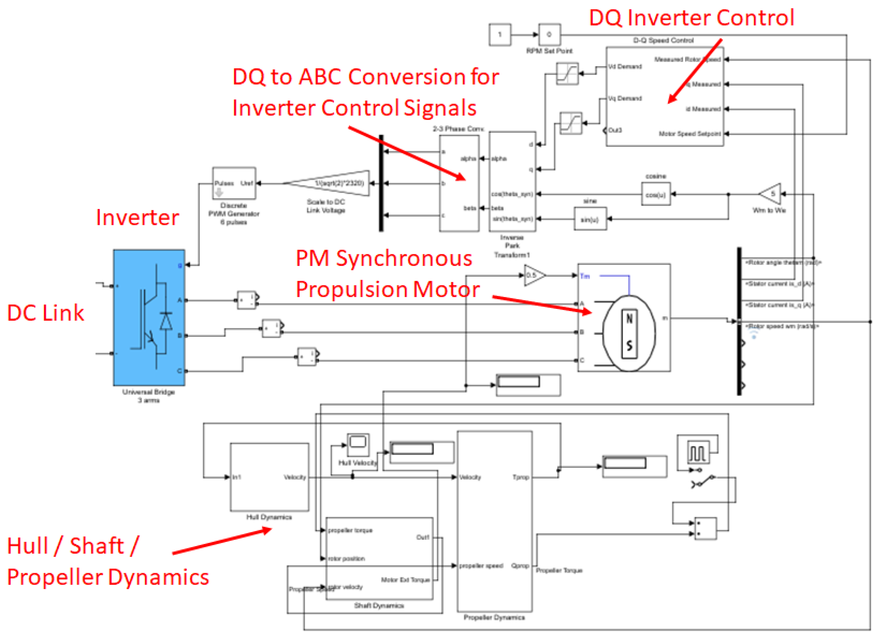
2.9. Inverter/Motor Drive
2.10. Hull Characteristics/Propellor Shaft Dynamics
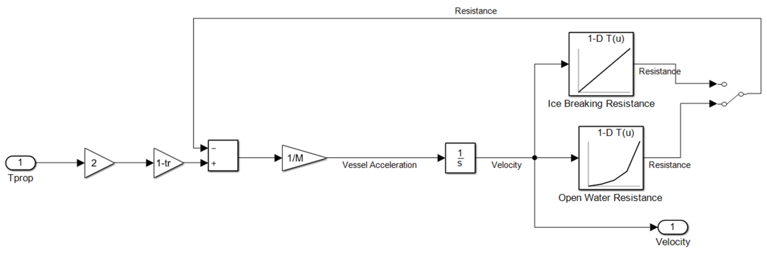
2.11. Hull Dynamics
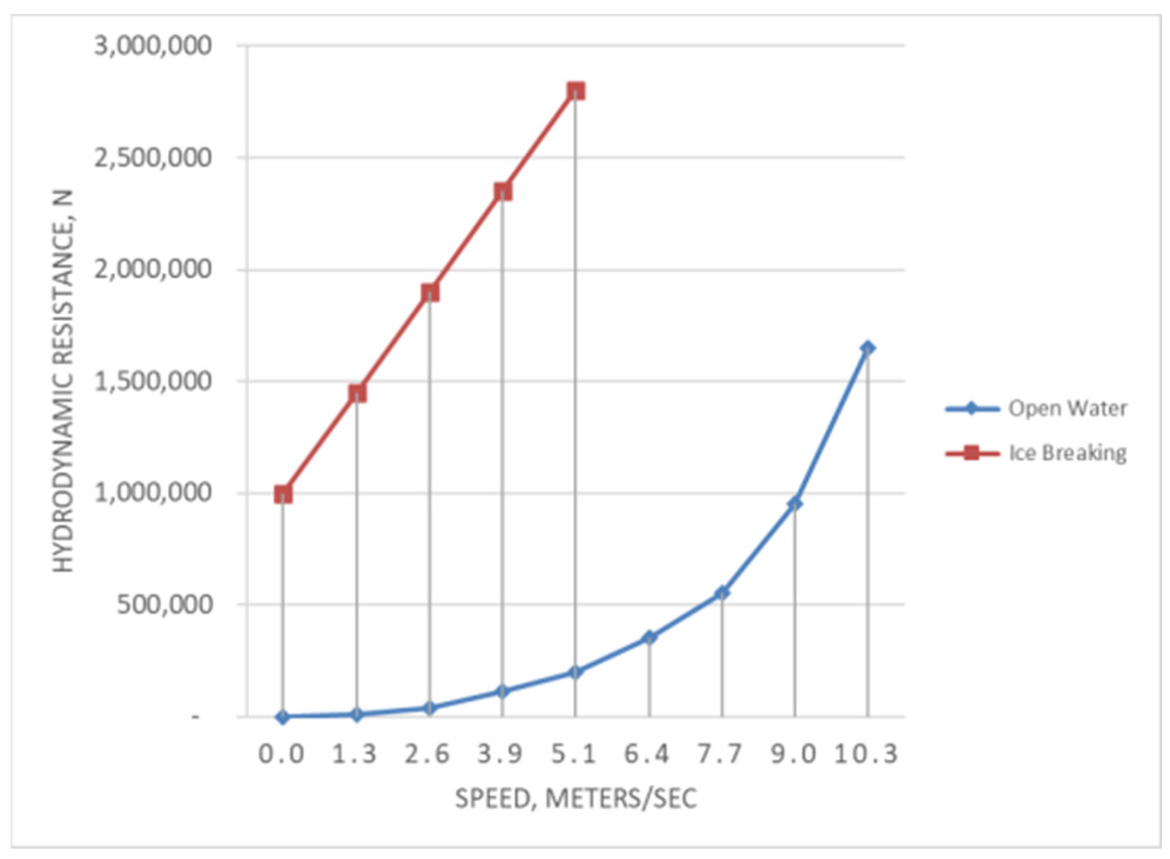
2.12. Hydrodynamic Resistance
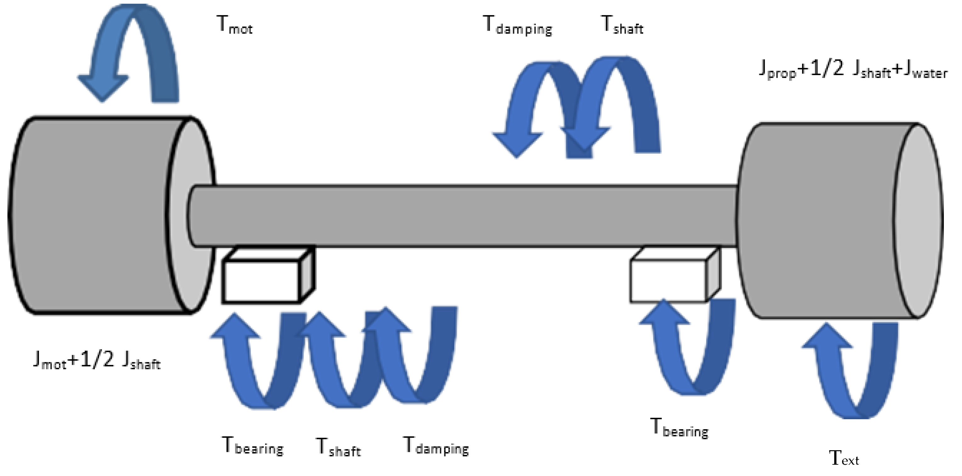
2.13. Shaft & Propeller Dynamics
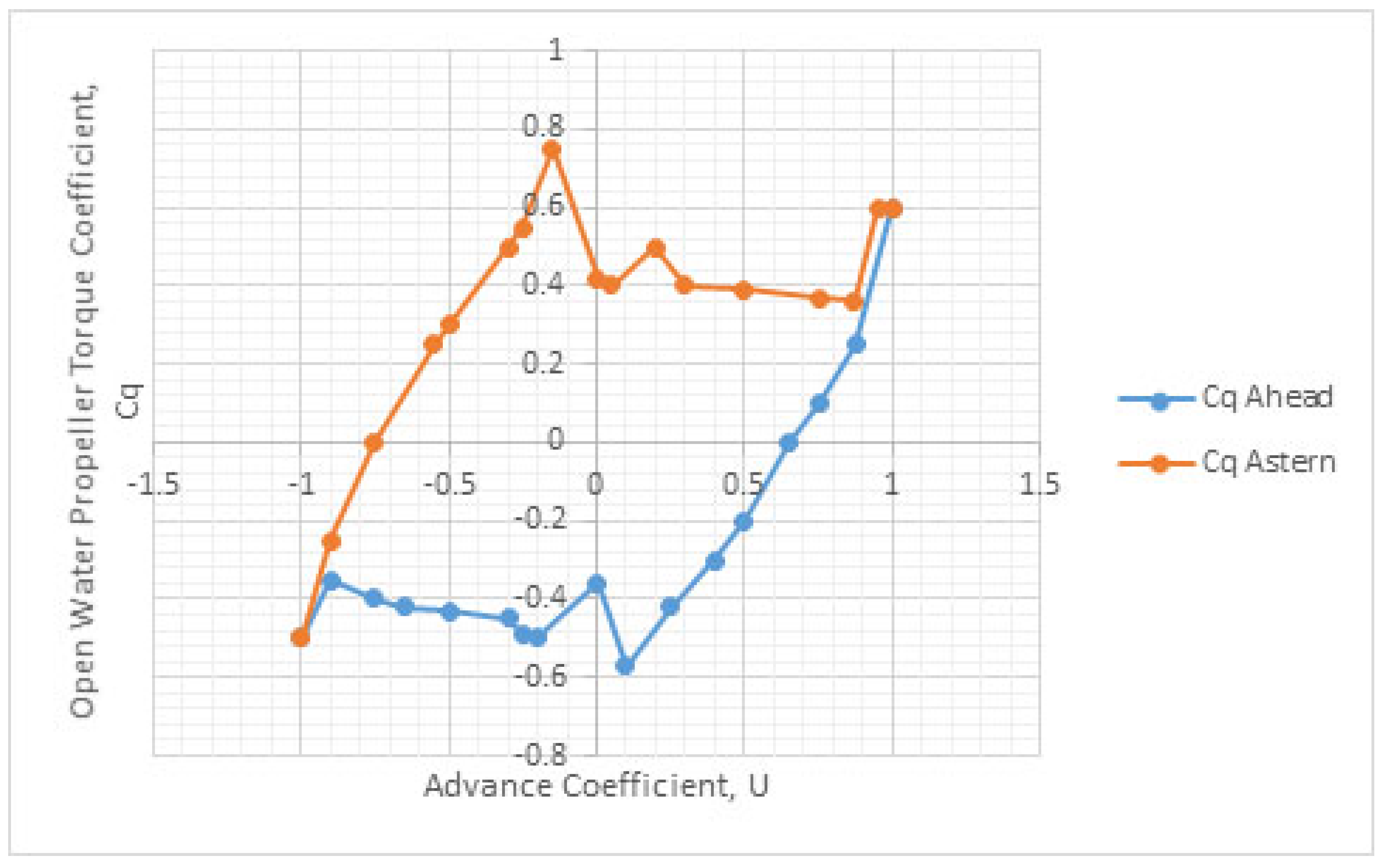
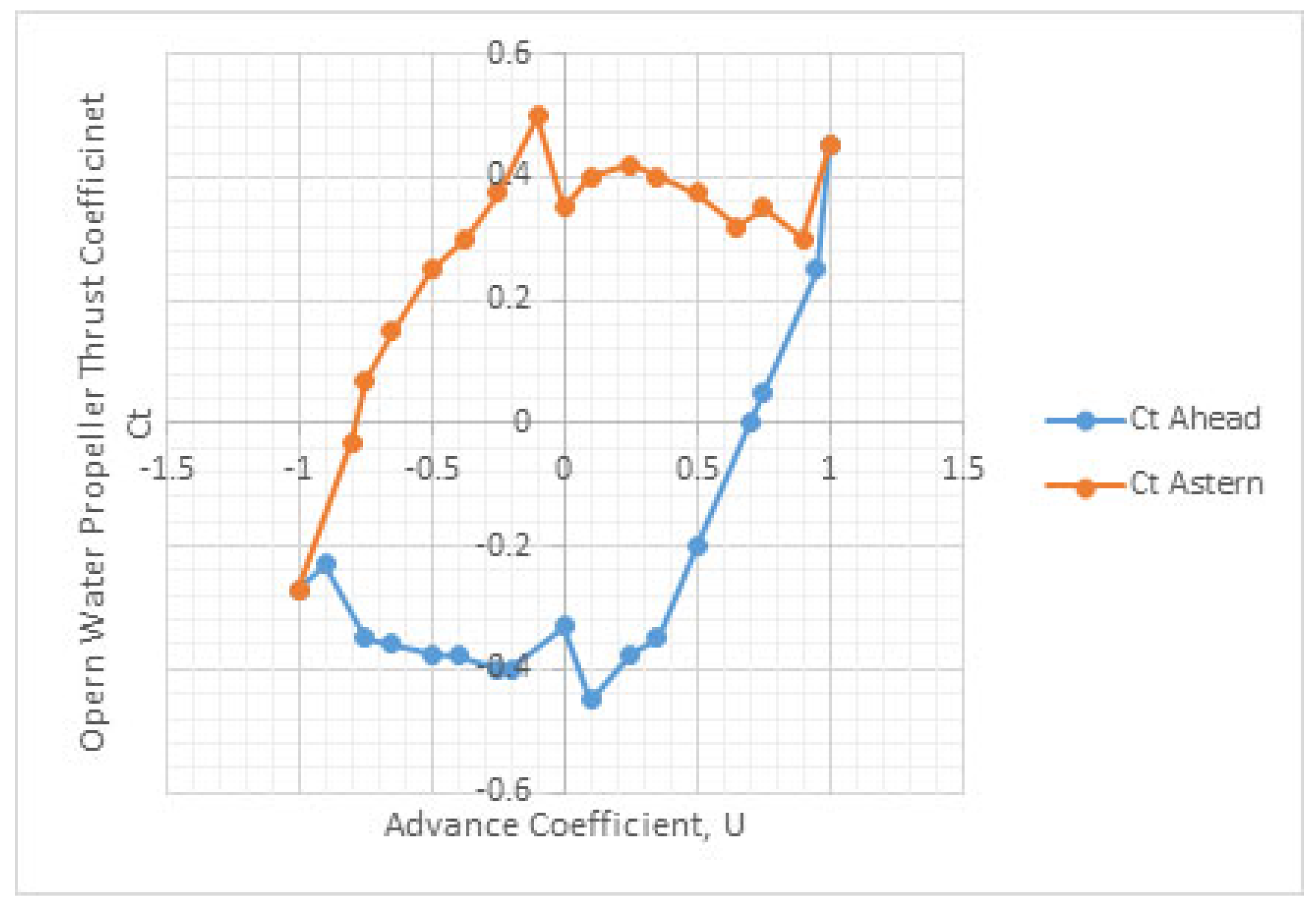
2.14. Hydrodynamic Propeller Torque and Thrust
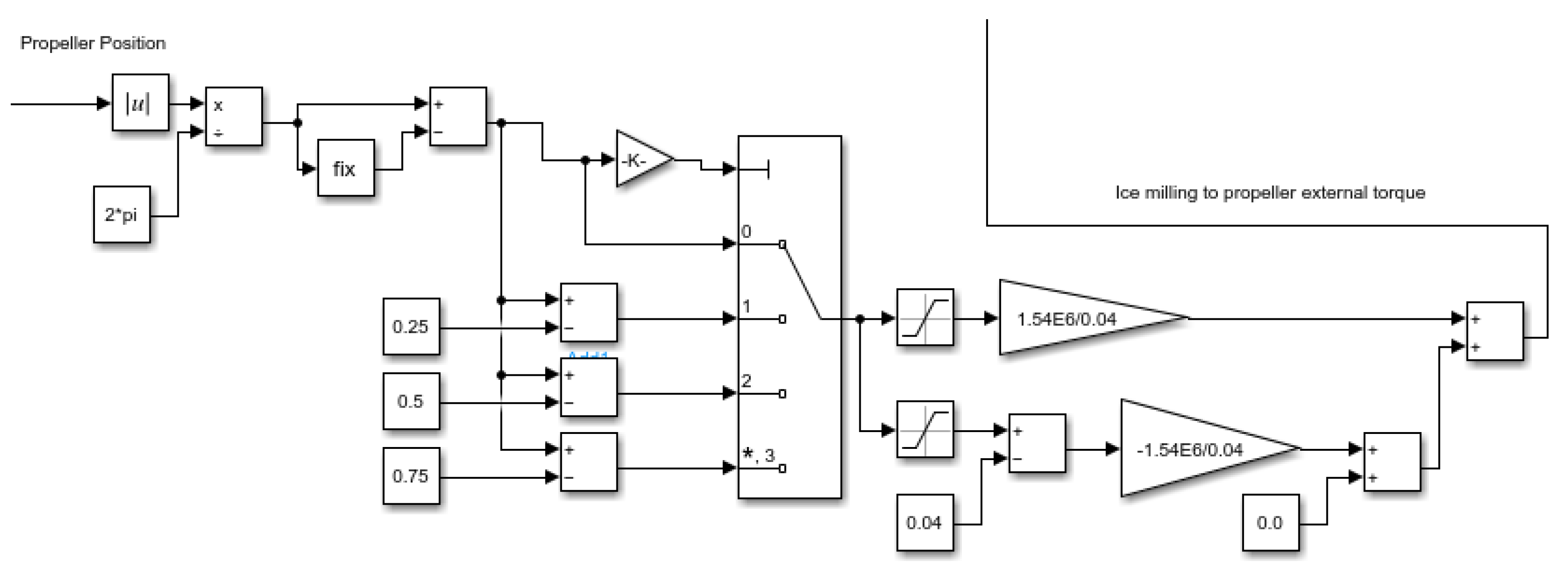
2.15. Ice Milling Torque
3. Results
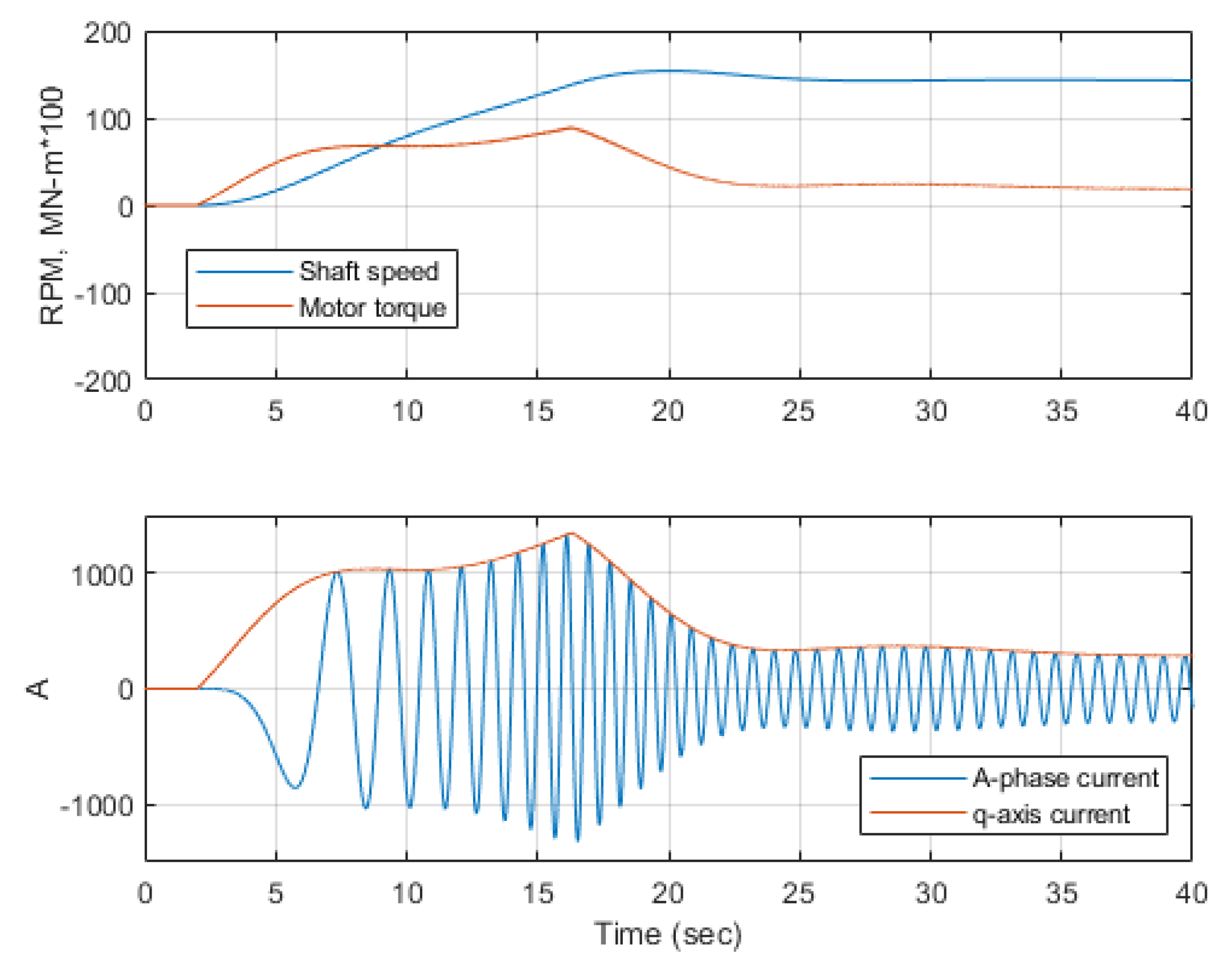
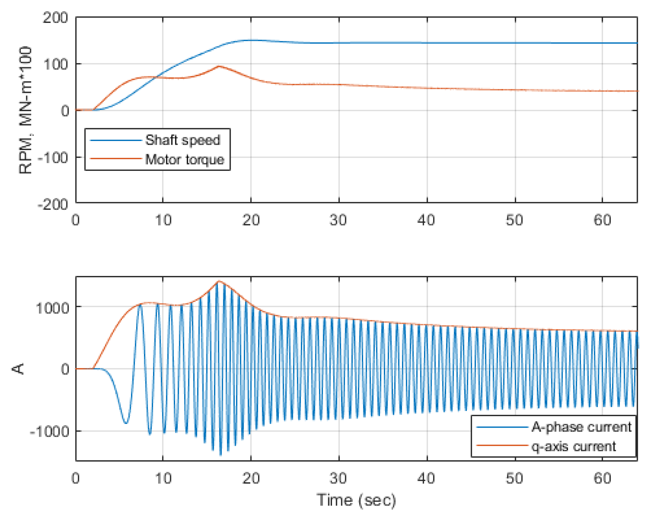
3.1. Ahead Operation
3.2. Harmonic Distortion
3.3. Ice Breaking
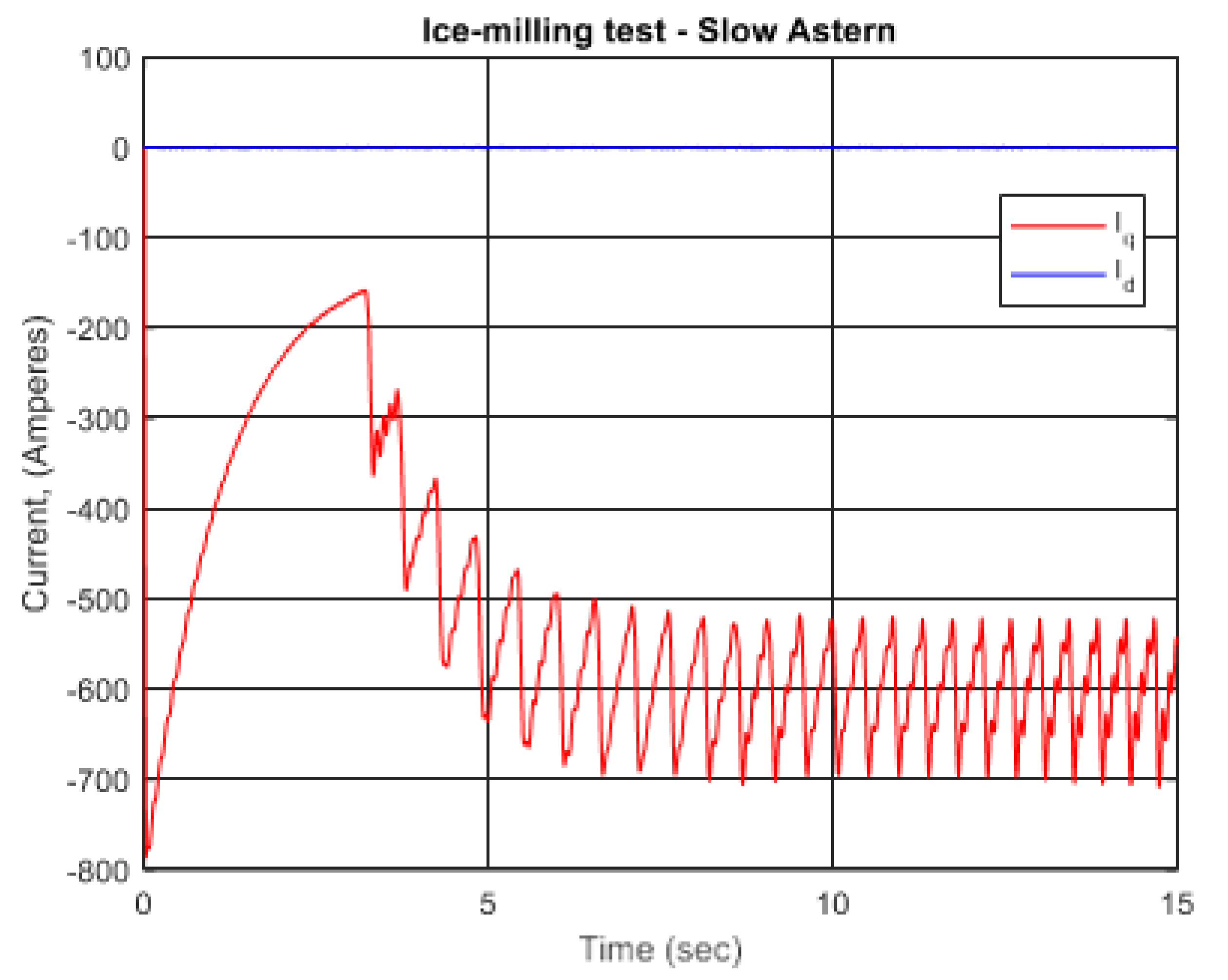
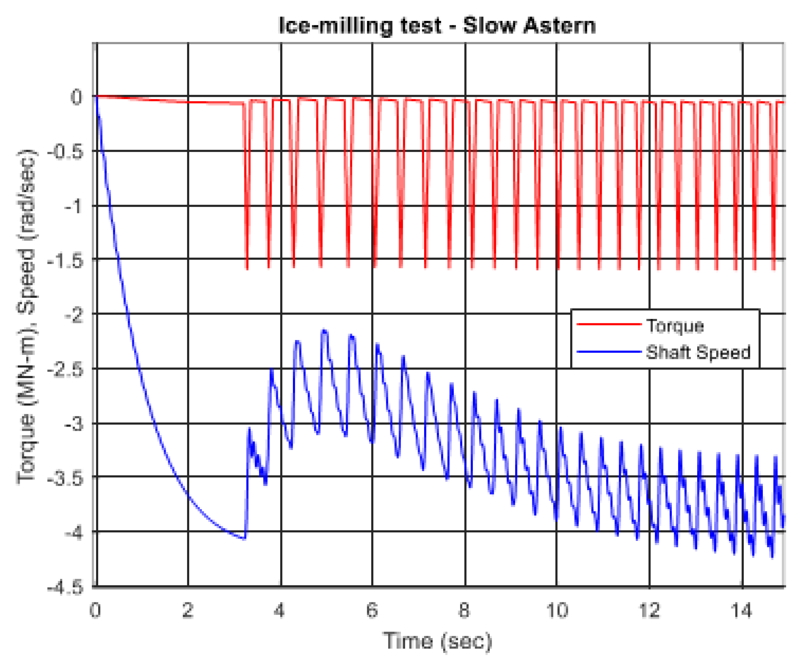
3.4. Ice Milling
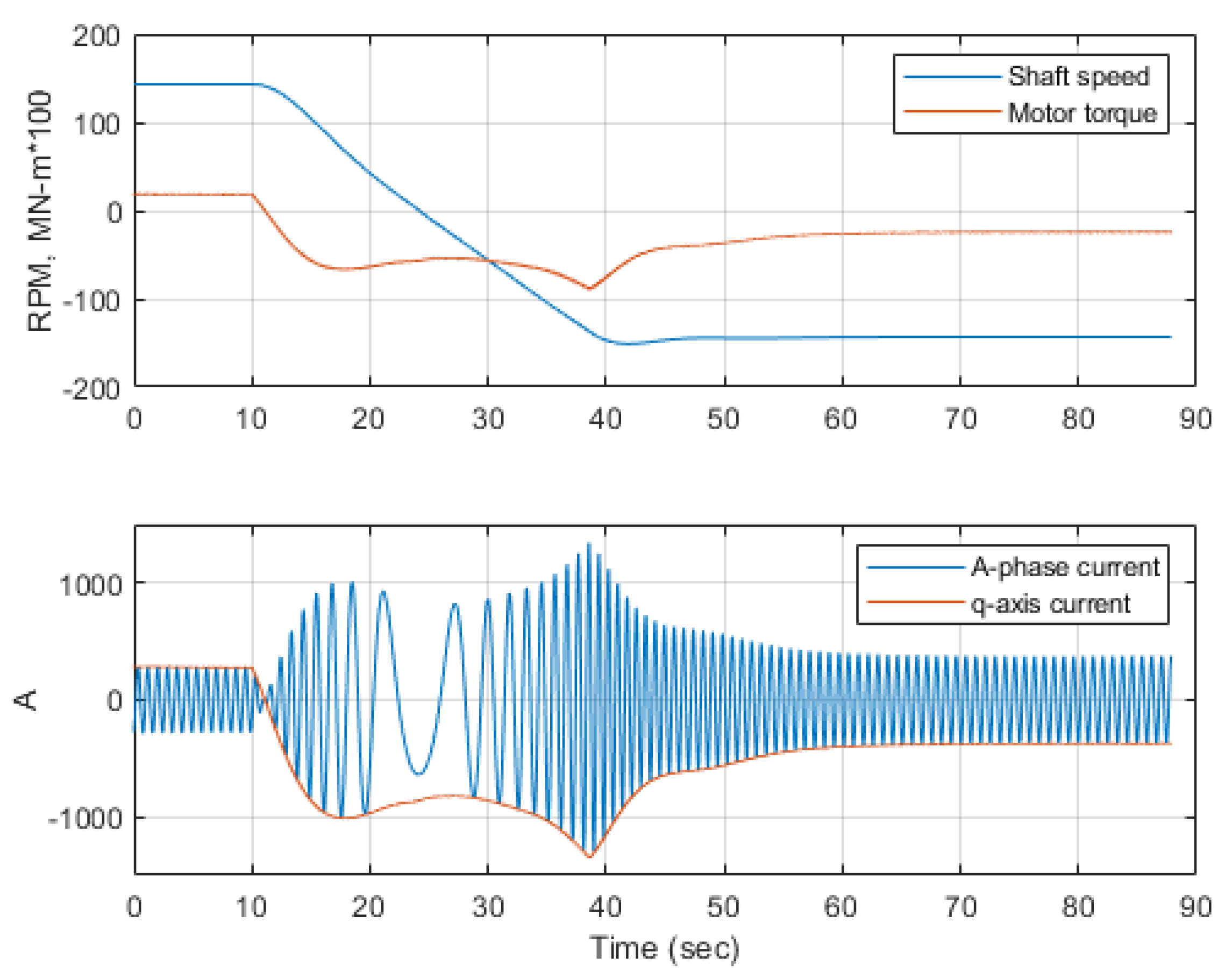
3.5. Crash Back (Emergency Crash Astern)
4. Discussion
Author Contributions
Funding
Data Availability Statement
Conflicts of Interest
References
- John, A. Beverley, Chapter VIII Electric Propulsion Drives. In Marine Engineering; Roy, L.H., Ed.; Society of Naval Architects and Marine Engineers: Jersey City, NJ, USA, 1992. [Google Scholar]
- Ned, M. Electric Machines and Drives, A First Course; John Wiley & Sons, Inc.: Hoboken, NJ, USA, 2012. [Google Scholar]
- Lecourt, E.J., Jr. Using Simulation to Determine the Maneuvering Performance of the WAGB-20. Nav. Eng. J. 1998, 110, 171–188. [Google Scholar] [CrossRef]
- Krause, W.; Sudhoff, P. Analysis of Electric Machinery and Drive Systems, 3rd ed.; Wiley: Hoboken, NJ, USA, 2013. [Google Scholar]
- Chester, L. Long, Chapter X Propellers, Shafting, and Shafting System Vibration Analysis. In Marine Engineering; Roy, L.H., Ed.; Society of Naval Architects and Marine Engineers: Jersey City, NJ, USA, 1992. [Google Scholar]


Publisher’s Note: MDPI stays neutral with regard to jurisdictional claims in published maps and institutional affiliations. |
© 2022 by the authors. Licensee MDPI, Basel, Switzerland. This article is an open access article distributed under the terms and conditions of the Creative Commons Attribution (CC BY) license (https://creativecommons.org/licenses/by/4.0/).
Share and Cite
Renz, E.C.; Turso, J. Toward the Application of Pulse Width Modulated (PWM) Inverter Drive-Based Electric Propulsion to Ice Capable Ships. Energies 2022, 15, 8217. https://doi.org/10.3390/en15218217
Renz EC, Turso J. Toward the Application of Pulse Width Modulated (PWM) Inverter Drive-Based Electric Propulsion to Ice Capable Ships. Energies. 2022; 15(21):8217. https://doi.org/10.3390/en15218217
Chicago/Turabian StyleRenz, Eric Christopher, and James Turso. 2022. "Toward the Application of Pulse Width Modulated (PWM) Inverter Drive-Based Electric Propulsion to Ice Capable Ships" Energies 15, no. 21: 8217. https://doi.org/10.3390/en15218217
APA StyleRenz, E. C., & Turso, J. (2022). Toward the Application of Pulse Width Modulated (PWM) Inverter Drive-Based Electric Propulsion to Ice Capable Ships. Energies, 15(21), 8217. https://doi.org/10.3390/en15218217