Performance Prediction and Working Fluid Active Design of Organic Rankine Cycle Based on Molecular Structure

Abstract

Working fluid selection is crucial for organic Rankine cycles (ORC). In this study, the relationship between molecular structure and ORC performance was established based on the quantitative structure–property relationship (QSPR) and working fluid parameterized model (WFPM), from which an ORC working fluid was actively designed. First, the QSPR model with four properties, namely, critical temperature (T_c), boiling point (T_b), critical pressure (p_c), and isobaric heat capacity ($c_{\mathrm{p}}^0$), was built. Second, the evaporation enthalpy (h_vap), evaporation entropy (s_vap), and thermal efficiency (η) were estimated by WFPM, and the results were compared with those using REFPROP to verify the calculation accuracy of the “QSPR+WFPM” coupling model. The average absolute relative deviations of evaporation enthalpy and entropy are below 8.44%. The maximum relative error of thermal efficiency is 6%. Then, the thermodynamic performance limit of ORC and corresponding thermophysical properties of the ideal working fluid were calculated at typical geothermal source conditions. Finally, the active design of the working fluid was conducted with the ideal working fluid T_c and p_c as the target. The research shows that C₃H₄F₂ and C₄H₃F₅ are optimal working fluids at 473.15 and 523.15 K heat sources, respectively.

1. Introduction

Environmental and energy issues are severe at present. Therefore, improving the utilization efficiency of low-grade thermal energies, such as solar energy [1], geothermal energy [2], and internal combustion engine waste heat [3], is an important means to alleviate the global climate change and energy crisis. The conversion of low-grade thermal energy into electrical energy at present is mainly achieved through the thermodynamic cycle. The Organic Rankine cycle (ORC) has a simple structure, a wide applicable heat source temperature range, and convenient maintenance. It has been widely used in the utilization of low-grade thermal energy. ORC realizes the conversion of heat and power through the change in the thermodynamic state of the working fluid. Selecting an appropriate working fluid can improve the performance of ORC. Thus, working fluid selection is a major research area in the field of ORC.

1.1. Working Fluid Selection

The working fluid selection can be divided into a passive selection and an active design. Passive selection is a traditional method in which one or more working fluids are selected from a given working fluid pool under the given conditions. Stijepovic et al. [4] analyzed the effects of the compressibility factor, ideal isobaric heat capacity, molecular weights, and other thermophysical properties of the working fluid on the economic and thermodynamic performance of ORC. They also provided a reference for working fluid selection. Hu et al. [5] selected the working fluid for ORC driven by geothermal energy. The net power output per unit mass of geothermal water was selected as the evaluation index to evaluate the system’s performance. The results showed that R245fa was the optimal working fluid. Quoilin et al. [6] studied the working fluids in ORC from a technical and economical viewpoint. The investigated working fluids included R245fa, R123, R1234yf, Solkatherm, n-butane, and n-pentane. The results showed that the optimal working fluid varied with the optimization objective. The existing research cannot obtain an optimal working fluid to meet the requirements of different temperatures and working conditions. Ping et al. [7] selected R245fa to analyze the dynamic corresponding characteristics of ORC under different driving cycles. Abbas et al. [8] selected cyclohexane and cyclopentane from 37 working fluids. The ORC efficiency can reach 19.13% and 18.03% when using the two working fluids, respectively. In addition, some researchers conducted a theoretical analysis of the number of working fluids, and several indicators were proposed for working fluid selection, such as a critical temperature [9], boiling point [10], or several property combinations [11].

Working fluid passive selection promotes the progress of ORC technology, but it still has limitations. Owing to the fact that the working fluid can only be found in a given working fluid pool, the working fluid that is not included cannot be selected and evaluated. Compared with passive selection, the active design does not need to give the working fluid pool in advance. Only a few molecular groups are required to generate a large number of working fluids, from which an optimal working fluid can be selected. Computer-aided molecular design (CAMD) is a common method for working fluid active design; it has been used in the fields of pharmacy and refrigeration; it also synthesizes specific function drugs [12] and refrigerants [13]. In recent years, some researchers have introduced CAMD into the working fluid design of ORC. For the novel working fluids designed by CAMD, the corresponding performance in ORC could not be calculated by REFPROP or COOLPROP. Therefore, a reliable ORC performance prediction model needs to be established to solve this problem. Su et al. [14,15] adopted a group contribution method to predict seven kinds of thermophysical properties, such as the boiling point, critical properties, and acentric factor. The proposed method achieved reliable results. Meanwhile, they estimated the net output work and thermal efficiency of ORC based on the semi-empirical formula. In their subsequent works, the novel working fluids R254eb and R254cb were proposed under given working conditions based on the group contribution method. Chen et al. [16] used cubic equations of state (EoS) instead of semi-empirical formulas to predict the performance of subcritical basic ORC and subcritical regenerative ORC. The working fluids were designed for a different ORC. Brown et al. [17] combined the group contribution method with Peng–Robinson EoS to rapidly evaluate the performance of ORC. Lampe et al. [18] combined QSPR and the perturbed-chain statistical associating fluid theory (PC-SAFT) to propose an overall design framework for ORC application, which could optimize the working fluid and process parameters simultaneously.

The prediction model is generally composed of two parts: thermophysical property prediction and ORC performance calculation. In our previous work [19,20,21], the working fluid parameterized model (WFPM) was proposed to calculate ORC performance. However, this model has not been applied to novel working fluids.

1.2. Thermophysical Property Prediction and Molecular Design

The ORC performance is greatly affected by the thermophysical properties of the working fluid. Obtaining accurate thermophysical properties of the working fluid is significant work, and experiment is an important method, but experiments are laborious. Researchers began to focus on the molecular structure to explore an efficient method for obtaining thermophysical properties of the working fluid due to a strong correlation between them. The quantitative structure–property relationship (QSPR) is a method to find the relationship between thermophysical properties and molecular structure and establish a mathematical relationship between them. QSPR has been widely used in biology, chemistry, and other fields. The activity of enzymes and the toxicity of compounds can be predicted by this method. At present, some researchers have used this method to predict the thermophysical properties of the organic working fluid. Abudour et al. [22] established the QSPR model to predict the binary interaction coefficient of PR EoS based on the characteristic parameters of molecular structure. Abooali et al. [23] established a five-variable boiling point model and a six-variable evaporation enthalpy multiple linear regression model. The molecular descriptors were selected through the enhanced replacement method. The results showed that the average absolute deviations were 3.42% and 6.83%. Banchero et al. [24] used a radial basis function neural network and multiple linear regression to establish QSPR model of critical temperature, critical pressure, and acentric factor of organic compounds. The results showed a strong relationship between the properties and descriptors characterizing electron charge distribution in the molecule. The group contribution method is part of the QSPR method. The macroscopic properties are regarded as the sum of the contributions of each group. The method is also widely applied in the prediction of the thermophysical properties of the working fluid. Joback [25] used the group contribution method to predict the properties of pure components. Lan et al. [26] utilized the group contribution method to analyze the T_c and p_c of mixed biofuels. The results showed that the method had high accuracy.

Inverse QSPR (i-QSPR) is an inverse process searching for molecular structure by properties. The relationship between QSPR and i-QSPR is shown in Figure 1. Weis et al. [27] used the boiling point and gas-phase thermal conductivity of R-141b as the property target of organic compounds to obtain an environmentally friendly hydrofluoroether foam blowing agent as a substitute for R-141b. They obtained seven candidate organic compounds adopting a signature molecular descriptor [28,29]. Lim et al. [30] conducted the molecular design with the molecular weight, partition coefficient, number of hydrogen bond donors, and other properties as the target properties of the drug molecules. The errors between the properties of the designed drug molecules and those of the target molecules were below 10%. Other researchers used i-QSPR to find novel drugs [31] and chemical structures [32].

QSPR can build a bridge from the molecular structure to thermophysical properties, which enables the design of the working fluids of ORC. However, studies that combine the working fluids of ORC with QSPR are rarely reported, and further research is required in this field.

1.3. Contribution of This Work

Passive selection cannot support the further development of ORC technology due to its limits. Meanwhile, an active design can overcome those limits and find potential and preferable working fluids for ORC. Thus, it has become an important method in working fluid design. Studies on the combination of QSPR and working fluid design are few. If working fluid design and QSPR can be combined, then the novel ORC working fluids can be designed to maximize the performance of ORC. The main contributions to this study are listed as follows:

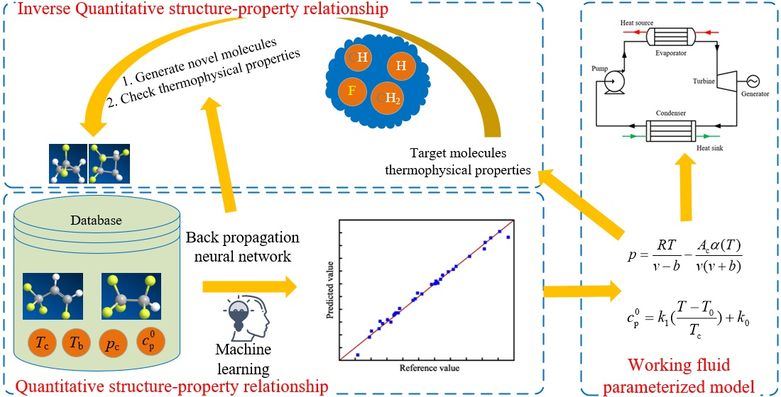
• The accurate prediction of thermophysical properties was realized based on the QSPR model.
• The evaporation enthalpy, evaporation entropy, and thermal efficiency of the working fluid were calculated, and the errors between the results of “QSPR+WFPM” and those of REFPROP were analyzed.
• The thermodynamic performance limits the ORC system, and the thermophysical properties of the ideal working fluid were investigated at typical geothermal source conditions. Working fluids were actively designed at the molecular scale on the basis of these properties.

The rest of the paper is organized as follows. In Section 2, WFPM is introduced based on the principle of the corresponding state. In Section 3, the QSPR model is built by BP neural network. In Section 4, the “QSPR+WFPM” coupling model is used to calculate the performance of ORC. In Section 5, the thermodynamic performance limit of ORC and the corresponding thermophysical properties of the ideal working fluid are calculated. The novel working fluid is actively designed by i-QSPR, taking the properties as the goal. In Section 6, the conclusions are given.

2. Theoretical Model

WFPM has been discussed in detail in our previous work [20]. The model is introduced briefly in this section. Four thermophysical properties (T_c, p_c, ω, and $c_{\mathrm{p}}^0$) were chosen to characterize the working fluids in our model. The thermodynamic properties are calculated by the Helmholtz free energy formula, and the free energy is derived from residual and ideal properties.

$$a(T,\rho ;{\theta }^{\mathrm{res}},{\theta }^0)=a^{\mathrm{res}}(T,\rho ;{\theta }^{\mathrm{res}})+a^0(T,\rho ;{\theta }^0)$$

(1)

The residual properties are calculated by an improved SRK EoS, and the equations are as follows:

$$p=\frac{RT}{v-b}-\frac{A_{\mathrm{c}}\alpha \left(T\right)}{v(v+b)}$$

(2)

$$A_{\mathrm{c}}=0.42747\frac{R^2{T}_{\mathrm{c}}^2}{p_{\mathrm{c}}}$$

(3)

$$b=0.08664\frac{R{T}_{\mathrm{c}}}{p_{\mathrm{c}}}$$

(4)

$$\alpha (T)=\{\begin{array}{l}{[1+m(1-\sqrt{T_{\mathrm{r}}})]}^{12},T\mathrm{r}\le 1\\ \exp [a_1(T\mathrm{r}-1)+a_2{(\sqrt{T\mathrm{r}}-1)}^2+a_3{(\sqrt[3]{T\mathrm{r}}-1)}^3],T\mathrm{r}>1\end{array}$$

(5)

$$T_{\mathrm{r}}=\frac{T_{\mathrm{b}}}{T_{\mathrm{c}}}$$

(6)

$$m=0.480654+1.55402\omega -0.123957{\omega }^2$$

(7)

The ideal gas thermodynamic properties are obtained by integrating $c_{\mathrm{p}}^0$. $c_{\mathrm{p}}^0$ and is given by:

$$c_{\mathrm{p}}^0=k_1(\frac{T-T_0}{T_{\mathrm{c}}})+k_0$$

(8)

The working fluid can be characterized by critical properties, the acentric factor, and isobaric specific heat. The model has been verified on the working fluid and ORC system levels, which proves the accuracy of the model.

3. QSPR Modeling

As mentioned in Section 2, the WFPM involves constants A_c, b, α(T), and m, which can be calculated from thermophysical properties of the working fluid (T_c, p_c, ω, and $c_{\mathrm{p}}^0$). In this study, QSPR was used to predict the thermophysical properties. The progress of QSPR included the following three steps: (1) data collection; (2) molecular descriptor calculation and selection; (3) model establishment and evaluation.

A more intuitive inherent property T_b is used to replace ω, and the conversion formula between T_b and ω is as follows [33]:

$$\omega =\frac{0.3(0.2803+0.4789T_{\mathrm{r}})\lg p_{\mathrm{c}}}{(1-T_{\mathrm{r}})(0.9803-0.5211T_{\mathrm{r}})}-1$$

(9)

3.1. Data Collection

Selecting an accurate and representative dataset is a critical step in developing QSPR models [34,35]. In this study, T_c, p_c, and T_b of 220 organic compounds and $c_{\mathrm{p}}^0$ under 298.15 K of 166 organic compounds were collected. The data were all obtained from NIST [36]. The organic compounds included halogenated hydrocarbons, alcohols, and aromatic groups, of which the ranges of T_c, p_c, T_b, and $c_{\mathrm{p}}^0$ were 292.8–805.09 K, 1.2–13.3 MPa, 188.7–634.2 K, and 37.45–485.83 kJ·kmol⁻¹·K⁻¹, respectively.

3.2. Molecular Descriptor Calculation and Selection

Aiming at the analysis of QSPR with a mathematical method, molecular structures are often characterized by molecular descriptors, which can convert molecular structures into precise mathematical values. Considerable professional software is applied for calculating molecular descriptors. In this study, AlvaDesc was used, which can calculate 5666 descriptors, including connectivity indices, topological indices, geometrical descriptors, pharmacophore descriptors, and 33 other types of descriptors to characterize the important features of the molecules.

When using AlvaDesc, the molecular structures in the dataset are imported into AlvaDesc to calculate the descriptors for all the molecules. Molecular descriptors can have strong correlations with others, which require a preliminary selection. The selection steps are as follows: (1) delete “Constant values” and “Near constant values”; (2) delete “At least one missing value”; (3) delete “Pair correlation larger or equal to 0.9”. After preliminary selection, 423 molecular descriptors are retained.

A further selection is needed to determine the molecular descriptors that are closely related to the thermophysical properties among the 423 molecular descriptors. In this study, a stepwise regression method was used for further selection. The main purpose of the stepwise regression method is to select the most crucial variables from a large number of available variables. The specific method is to introduce the independent variables in sequence, and the condition of this introduction is that the partial regression sum of the squares is significant after testing. At the same time, the old independent variables should be tested in sequence each time a new independent variable is introduced, and the independent variables with an insignificant partial regression sum of squares should be eliminated. Through this method, 10 molecular descriptors were selected for each property [23], as listed in

Table 1. Molecular descriptors of T_c, T_b, p_c, and $c_{\mathrm{p}}^0$ QSPR model.

Property	Descriptor	Group
Tc	X3sol	Connectivity indices
	CATS2D_00_DD	Pharmacophore descriptors
	F06[C-O]	2D Atom Pairs
	SHED_AL	Pharmacophore descriptors
	Eta_D_AlphaB	eta delta alpha b index
	GATS1e	2D autocorrelations
	SpMaxA_AEA(bo)	Edge adjacency indices
	X2sol	Connectivity indices
	Eta_betaP_A	ETA indices
	NssCH2	Atom-type E-state indices
pc	SM5_D/Dt	2D matrix-based descriptors
	CATS2D_07_AL	Pharmacophore descriptors
	Hy	Molecular properties
	F06[C-N]	2D Atom Pairs
	CMC-80	Drug-like indices
	piPC10	Walk and path counts
	SpMin7_Bh(s)	Burden eigenvalues
	GATS1e	2D autocorrelations
	P_VSA_charge_8	P_VSA-like descriptors
	B06[C-N]	2D Atom Pairs
Tb	X3sol	Connectivity indices
	CATS2D_00_DD	Pharmacophore descriptors
	HVcpx	Information indices
	F06[C-N]	2D Atom Pairs
	GATS1e	2D autocorrelations
	X2sol	Connectivity indices
	nRCN	Functional group counts
	SpMAD_Dz(v)	2D matrix-based descriptors
	F06[C-O]	2D Atom Pairs
	Chi1_EA(dm)	Edge adjacency indices
$c_{\mathrm{p}}^0$	TIC3	Information indices
	SpMAD_Dz(v)	2D matrix-based descriptors
	ATSC4m	2D autocorrelations
	RNCG	Charge descriptors
	J_Dz(p)	2D matrix-based descriptors
	GATS2m	2D autocorrelations
	JGI5	2D autocorrelations
	Chi1_EA(dm)	Edge adjacency indices
	phLevel1	Chirality descriptors
	Eig11_AEA(bo)	Edge adjacency indices

. A detailed explanation of the molecular descriptors is referred to on the website of AlvaDesc [37].

3.3. Model Establishment and Evaluation

BP neural networks have been widely used in QSPR due to their excellent nonlinear mapping ability and prediction performance. In this study, a three-layer BP neural network was selected to predict the thermophysical properties of the working fluids. The input parameters of the BP neural network are molecular descriptors, and the output parameters are prediction properties. The proportions of the training, validation and test sets were 70%, 15%, and 15%, respectively [38]. The transfer functions of the hidden and output layers of the BP neural network are tansig and purelin. Levenberg–Marquardt was selected as an optimization function. The optimal node numbers were determined as 15 by comparing the node numbers in the different hidden layers. The schematic of the BP neural network structure is shown in Figure 2.

Two statistical parameters, namely, the average absolute relative deviation (AARD) and the root mean square error (RMSE), were used as the evaluation indexes of the BP neural network. The AARD and RMSE are defined as:

$$\mathrm{AARD}=\frac{1}{n}{\displaystyle \sum _{i=1}^n\left|\frac{y_{\mathrm{i},\mathrm{NIST}}-y_{\mathrm{i},\mathrm{cal}}}{y_{\mathrm{i},\mathrm{NIST}}}\right|\times 100}$$

(10)

$$\mathrm{RMSE}=\sqrt{\frac{1}{n}{\displaystyle \sum _{i=1}^n{(y_{\mathrm{i},\mathrm{cal}}-y_{\mathrm{i},\mathrm{NIST}})}^2}}$$

(11)

where n is the sum of calculated data, $y_{\mathrm{i},\mathrm{NIST}}$ represents the properties from NIST, and $y_{\mathrm{i},\mathrm{cal}}$ represents the calculated properties.

The comparisons of T_c in the training, validation, and test set are shown in Figure 3a–c, respectively. Their correlation coefficients are 0.9923, 0.9866, and 0.9883, respectively, which prove that the BP neural network exhibits an excellent performance. The comparisons of other properties are shown in Appendix A. The statistical parameters of the four properties are listed in

Table 2. Comparison of the statistical parameters for four properties.

Properties		Training Set	Validation Set	Test Set	Total Set
Tb	Data point	152	32	32	216
	AARD/(%)	1.9381	2.0381	2.9517	2.1031
	RMSE	8.3961	9.2421	13.0771	9.3593
Tc	Data point	152	32	32	216
	AARD/(%)	2.0331	2.0293	1.8869	2.0109
	RMSE	13.8645	12.7925	14.0122	13.7332
pc	Data point	152	32	32	216
	AARD/(%)	3.5374	3.6892	4.4833	3.6837
	RMSE	0.2204	0.2066	0.2138	0.2169
$c_{\mathrm{p}}^0$	Data point	114	24	24	162
	AARD/(%)	7.2998	8.9453	13.4422	8.4536
	RMSE	11.3718	18.9047	23.0043	14.9113

. The model of $c_{\mathrm{p}}^0$ has a low accuracy but is within the acceptable range. Meanwhile, the models of T_c, p_c, and T_b have a better prediction accuracy.

Table 3. Prediction accuracy comparison between this work and the other literatures.

	RMSE
	Tc (K)	pc (MPa)	Tb (K)	$$\begin{gathered} {\mathit{c}}_{\mathbf{p}}^0 \\ (\mathbf{kJ}·{\mathbf{kmol}}^{-1}·{\mathbf{K}}^{-1}) \end{gathered}$$
This work	13.7	0.22	9.36	8.45
Mauro Banchero et al. [24]	8.8	0.13	-	-
Gabriela Espinosa et al. [39]	30.2	0.3	27.7	-
Farhad Gharagheizi et al. [40]	17.7	0.17	-	-

lists the RMSE comparison with results of the other literature using ANN to predict working fluids’ thermophysical properties, indicating that the proposed model has an accepted prediction performance.

The prediction model of the evaporation enthalpy, evaporation entropy, and thermal efficiency of ORC can be established using the prediction results of the properties by QSPR as the input parameter of WFPM. The model is called the “QSPR+WFPM” coupling model. Its calculation process is shown in Figure 4.

4. Model Validation

Four commonly used ORC working fluids, namely, R245fa, R600a, R134a, and R1234ze(E), were selected to verify the accuracy of the “QSPR+WFPM” coupling model. They are not included in the QSPR dataset.

Table 4. RE of four working fluid properties.

Working Fluid		Tc (K)	pc (MPa)	$$\begin{gathered} {\mathit{c}}_{\mathbf{p}}^0 \\ (\mathbf{J}·{\mathbf{mol}}^{-1}·{\mathbf{K}}^{-1}) \end{gathered}$$	Tb (K)	ω
R600a	NIST	407.70	3.65	96.64	262.00	0.1840
	Calculated	402.20	3.80	84.83	264.14	0.2565
	RE(%)	−1.35	4.10	−12.22	0.82	39.40
R245fa	NIST	427.01	3.65	115.28	288.20	0.3783
	Calculated	425.44	3.40	112.91	288.48	0.3756
	RE(%)	−0.37	−6.85	−2.06	0.10	−0.71
R134a	NIST	374.10	4.06	85.03	246.60	0.3268
	Calculated	370.30	4.04	89.66	241.43	0.2807
	RE(%)	−1.02	−0.49	5.45	−2.10	−14.11
R1234ze(E)	NIST	382.51	3.64	99.65	254.18	0.3130
	Calculated	398.29	3.62	95.50	261.29	0.2652
	RE(%)	4.13	−0.55	−4.16	2.80	−15.27

lists the relative error (RE) of the properties of the four working fluids, which are defined as:

$$\mathrm{RE}=\frac{y_{\mathrm{i},\mathrm{NIST}}-y_{\mathrm{i},\mathrm{cal}}}{y_{\mathrm{i},\mathrm{NIST}}}\times 100$$

(12)

4.1. Validation of Working Fluid Thermophysical Properties

h_vap and s_vap are calculated using the proposed model. Two statistical parameters, namely, AARD and the mean average error (MAE), were used as the validation indexes of “QSPR+WFPM”. The AARD and MAE are defined as:

$$\mathrm{AARD}=\frac{1}{n}{\displaystyle \sum _{i=1}^n\left|\frac{{\widehat{y}}_{\mathrm{i}}-y_{\mathrm{i}}}{y_{\mathrm{i}}}\right|\times 100}$$

(13)

$$\mathrm{MAE}=\frac{1}{n}{\displaystyle \sum _{i=1}^n\left|{\widehat{y}}_{\mathrm{i}}-y_{\mathrm{i}}\right|}$$

(14)

where n is the sum of calculated data, ${\widehat{y}}_{\mathrm{i}}$ is the calculation result of the “QSPR+WFPM” coupling model, and $y_{\mathrm{i}}$ is the calculation result of REFPROP.

The comparison with the calculated results of REFPROP is shown in Figure 5 and Figure 6. The figures show that h_vap and s_vap decrease with the increase in temperature, and AARDs are equal. The distribution of AARDs is different for the four working fluids. As listed in

Table 5. AARDs and MAEs of h_vap and s_vap.

		R245fa	R600a	R134a	R1234ze(E)
hvap	AARD (%)	1.51%	4.95%	5.61%	8.44%
	MAE (kJ·kg−1)	2.24	14.81	8.92	12.39
svap	AARD (%)	1.51%	4.95%	5.61%	8.44%
	MAE (kJ·kg−1·k−1)	0.0065	0.047	0.029	0.039

, the AARDs of the halogenated hydrocarbons R245fa and R134a are 1.51% and 5.61%, respectively. As shown in Table 4, the RE of the p_c of the working fluid R245fa is relatively large, and the RE of other thermophysical properties is relatively small. The AARD of h_vap and s_vap is small, which shows that p_c has little influence on h_vap and s_vap. For R134a, the errors of ω and $c_{\mathrm{p}}^0$ are relatively large, and the RE of other thermophysical properties is relatively small. The AARDs of h_vap and s_vap are relatively large, which indicates that ω and $c_{\mathrm{p}}^0$ have a greater influence on h_vap and s_vap. For the halogenated olefin R1234ze(E), its AARD is the largest, and the value is 8.44%. The calculated result of the proposed model is larger than that of REFPROP, which is mainly due to the fact that the calculated value of T_c is too high. For the alkane R600a, the AARD is 4.95%, and the calculation results of the proposed model and REFPROP intersect at around 360 K. Compared with other working fluids, the RE of ω and $c_{\mathrm{p}}^0$ is the largest, and the calculated value of ω is high, which indicates that ω affects the trends of h_vap and s_vap with temperature.

As shown in Figure 5 and Figure 6, the deviation of h_vap and s_vap is relatively large at some operating points, which is mainly caused by the superposition of errors in the QSPR and WFPM models. For QSPR, different machine-learning models can be tried, such as the support vector machine, the random tree, etc. For WFPM, other EoS, such as the modified cubic EoS and the PC-SAFT, can be tried. If the accuracy of both models is improved, the prediction will be further improved.

4.2. Verification of ORC System Performance

In this study, the thermal efficiency was selected for verification. The simple ORC system shown in Figure 7 was taken as an example to verify the ORC system, and its T–s diagram is shown in Figure 8. The working fluid undergoes four processes of expansion (1-2), condensation (2-4), compression (4-5), and evaporation (5-1) in turn to complete a cycle. The formula of the four processes and thermal efficiency are listed in

Table 6. Formula of ORC system.

Item	Thermodynamic Formula
Expansion process	${\dot{W}}_{\exp }=\dot{m}(h_1-h_2)$
Condensation process	${\dot{Q}}_{\mathrm{con}}=\dot{m}(h_2-h_4)$
Compression process	${\dot{W}}_{\mathrm{P}}=\dot{m}(h_5-h_4)$
Evaporation process	${\dot{Q}}_{\mathrm{eva}}=\dot{m}(h_1-h_5)$
Thermal efficiency	$\eta =\frac{{\dot{W}}_{\exp }-{\dot{W}}_{\mathrm{P}}}{{\dot{Q}}_{\mathrm{eva}}}$

. To avoid an overly complex simulation, the constraints and assumptions are defined as follows:

• The pressure and heat dissipation losses in the system components and pipelines are ignored.
• The whole system is in stable operation or operates at steady-state conditions.
• The isentropic efficiencies of the working fluid pump and expander are 0.65 [41] and 0.7 [42], respectively.
• The heat exchange capacity in the evaporator is 126 kW regardless of the limitation of the pinch point temperature difference between the actual heat source and the circulating working fluid.
• The evaporation temperature range is 323.15–0.9 T_c. The condensing temperature is 293.15–323.15 K. The superheat degree is 10 K.

A comparison of the thermal efficiency is shown in Figure 9. The figure shows that the thermal efficiency calculated by the proposed model was higher than that calculated by REFPROP for R245fa, R600a, and R1234ze(E), while that for R134a was lower than the thermal efficiency calculated by REFPROP. The average relative deviation (ARD) was used to evaluate the calculation results, and its expression is shown in Equation (15). The ARD of the four working fluids has the same trend of variation, which increases with the increase in temperature difference between T_eva and T_con. The distribution of ARD in the four working fluids is shown in Figure 10. R1234ze(E) has the largest ARD at 6%, which is mainly due to the large RE of T_c. Overall, the accuracy of the “QSPR+WFPM” coupling model is acceptable.

$$\mathrm{ARD}=\frac{1}{n}{\displaystyle \sum _{i=1}^n\frac{{\widehat{y}}_{\mathrm{i}}-y_{\mathrm{i}}}{y_{\mathrm{i}}}}\times 100$$

(15)

5. Method of Working Fluid Design

5.1. Optimization Problem

The functional relationship between the thermophysical properties and the thermal efficiency is obtained by WFPM. For the ORC system mentioned in Section 4.2, the optimization of ORC thermal efficiency at 473.15 and 523.15 K heat sources, T_eva, T_sup, and T_con were selected to characterize the cycle parameters, and T_c, p_c, T_b, and $c_{\mathrm{p}}^0$ were used to characterize the working fluid. η can be further expressed as:

$$\eta =f(T_{\mathrm{eva}},T_{\mathrm{con}},T_{\sup },T_{\mathrm{c}},p_{\mathrm{c}},T_{\mathrm{b}},c_{\mathrm{p}}^0)$$

(16)

The genetic algorithm (GA) is a computational model of biological evolution that simulates the natural selection and genetic mechanism of Darwinian biological evolution. At present, GA has become one of the widely used optimization algorithms and an important tool in the optimization of ORC [43,44]. This section uses the GA in the MATLAB optimization toolbox to solve the optimization problem. The requirements are to input the fitness function, namely, $\eta =f(T_{\mathrm{eva}},T_{\mathrm{con}},T_{\sup },T_{\mathrm{c}},p_{\mathrm{c}},T_{\mathrm{b}},c_{\mathrm{p}}^0)$, the constraint conditions and necessary parameter settings. The toolbox first generates and encodes a certain number of feasible solutions (T_eva, T_sup, T_con, T_c, p_c, T_b, $c_{\mathrm{p}}^0$). Then, the fitness assessment is conducted by the fitness function. Thereafter, the next-generation solutions are produced by the selection, crossover, and mutation operators according to the fitness and parameters (e.g., the crossover fraction and mutation rate). A flowchart of the optimization process is shown in Figure 11. The range of constraint conditions in the optimization model is listed in

Table 7. Variation range of characteristic parameters.

Parameter	Lower Limit	Upper Limit
Teva (K)	323.15	0.9Tc
Tsup (K)	0	20
Tcon (K)	293.15	323.15
Tc (K)	350	550
pc (MPa)	2	5
Tb (K)	110	310
$c_{\mathrm{p}}^0$ (J·mol−1·K−1)	60	250

, where the range of the working fluid characteristic parameters is determined according to the commonly used working fluids of ORC.

The parameter settings of the optimization model are significantly influenced by the optimization results. The optimization model requires verification before it can be optimized. The model parameters involved mainly the inclusion of population size, the selection function, the crossover factor, and the variation function. The parameter settings of the optimization algorithm determined in this study are listed in

Table 8. Parameter settings of genetic algorithm.

Parameter	Value
Population size	1000
Selection function	Tournament
Tournament size	10
Elite count	50
Crossover fraction	0.75
Mutation function	Adaptive mutation
Mutation rate	0.3
Maximum iteration number	500

, where the value of the parameter refers to our previous work [19,20].

Through this method, the thermodynamic performance limit of the simple ORC and the corresponding parameters are calculated, and the values are listed in

Table 9. Optimization results of simple ORC at typical geothermal source conditions.

Heat Sourse (K)	η (%)	Teva (K)	Tcon (K)	Tsup (K)	Tc,id (K)	pc,id (MPa)	Tb,id (K)	$$\begin{gathered} {\mathit{c}}_{\mathbf{p},\mathbf{id}}^0 \\ (\mathbf{kJ}·{\mathbf{kmol}}^{-1}·{\mathbf{K}}^{-1}) \end{gathered}$$
473.15	13.10	383.19	293.26	19.85	431.41	4.95	160.32	60.00
523.15	17.59	433.36	293.37	19.97	481.52	4.96	177.24	60.05

. In this study, the working fluid with thermophysical properties under the performance limit is called the ideal working fluid.

5.2. Working Fluid Active Design

In Section 5.1, the thermophysical properties of the ideal working fluid are calculated, but the existing working fluid pool may not possess such properties. Therefore, the active design of the working fluid is desired to be conducted by i-QSPR. Our target was to seek out candidate working fluids in order to replace the ideal working fluid based on the three properties of T_c, p_c, and T_b. However, the relationship between T_b and T_c is inconsistent with the common working fluids. In our previous study, the effect of T_c on thermal efficiency was much greater than that of T_b [21]. Thus, the constructions are only aimed at T_c and p_c. The main steps of the working fluid active design are described as follows:

• The generation of candidate working fluids. The elements in the periodic table that can be used as working fluids of ORC are limited [45]. In this study, six molecular groups were selected according to the working fluids commonly used in ORC, namely, –CH₂–, >C<, >C=, –F, –CH<, and –H. The maximum number of C atoms was set to four in order to simplify the calculation. Moreover, all working fluids including alkanes, alkenes, and cycloalkanes were generated under the constraints of chemical structure. A total of 244 candidate working fluids were obtained. The molecular descriptors of the candidate working fluids calculated by AlvaDesc, T_c,ca, and p_c,ca, were calculated by QSPR.
• The analysis of the thermophysical property error. In the process of the working fluid design, constructing a working fluid that exactly matches the two properties of the ideal working fluid is difficult. The RE between T_c,_ca and T_c,id is α, and the RE between p_c,ca and p_c,id is β. The values of α and β can be adjusted to obtain the candidate working fluid.

The process of the working fluid active design based on the two steps above is shown in Figure 12.

Table 10. Thermophysical properties and thermal efficiency of candidates at 473.15 K heat source.

Molecular Structure	Chemical Formula	Tc (K)	pc (MPa)	Tb (K)	$$\begin{gathered} {\mathit{c}}_{\mathbf{p}}^0 \\ (\mathbf{J}·{\mathbf{mol}}^{-1}·{\mathbf{K}}^{-1}) \end{gathered}$$	η (%)
	C3H4F2	432.52	4.80	294.80	30.63	12.98
	C3H3F3	429.03	4.36	283.36	60.97	12.83
	C3H4F2	436.83	4.31	303.06	35.30	12.22

and

Table 11. Thermophysical properties and thermal efficiency of candidates at 523.15 K heat source.

Molecular Structure	Chemical Formula	Tc (K)	pc (MPa)	Tb (K)	$$\begin{gathered} {\mathit{c}}_{\mathbf{p}}^0 \\ (\mathbf{J}·{\mathbf{mol}}^{-1}·{\mathbf{K}}^{-1}) \end{gathered}$$	η (%)
	C4H3F5	481.50	3.32	318.83	71.34	14.63
	C4H6F4	481.59	2.90	317.87	133.60	14.61
	C4H7F3	483.07	3.13	327.02	126.80	13.74

list the molecular structure and related thermophysical properties of the candidate working fluids under 473.15 and 523.15 K heat sources and the thermal efficiencies calculated by WFPM. The tables show that the thermal efficiencies of the constructed working fluids are similar to those of the ideal working fluid when the heat source temperature is 473.15 K. Table 10 and Table 11 list the molecular structure and related thermophysical properties of the candidate working fluids under 473.15 and 523.15 K heat sources, and the thermal efficiencies are calculated by WFPM.

The main reason for this, is that T_c,ca and p_c,ca are close to T_c,id and p_c,id. At the same time, T_b,ca is close to T_con. The expander inlet and outlet also have a large enthalpy difference. Thus, the expander has a large output power. However, these working fluids are halogenated cycloalkanes, which are rarely used in the ORC field. The reason for the large difference in the thermal efficiency of the constructed working fluid under a 523.15 K heat source is that T_b,ca is higher than T_con. The higher boiling point limits the expansion range of the working fluid, which results in the small output work of the expander.

The results of the working fluid active design show that no candidate working fluid has the same properties as the ideal working fluid. The difference between the candidate and ideal working fluid is mainly reflected in the boiling point. T_b,ca is much higher than T_b,id, which is the main reason why the thermal efficiency of the candidate working fluid is less than the thermodynamic performance limit.

Hitherto, there have been no relevant examples in the literature which have investigated the ORC performance of these candidate working fluids. However, the results of this study can provide the direction for the working fluid design of ORC in the future. Notably, the environmental protection and safety of the working fluid are important indicators for working fluid selection [46]. In this study, only the working fluid with optimal thermal efficiency was actively designed. The environmental and safety criteria for the proposed working fluids need to be further investigated.

6. Conclusions

In this study, four thermophysical properties of the working fluid (T_c, p_c, T_b, and $c_{\mathrm{p}}^0$) were predicted by the QSPR model. Based on these properties, evaporation enthalpy (h_vap), evaporation entropy (s_vap), and ORC thermal efficiency (η) were calculated by WFPM. These results were compared with those from REFPROP. By taking typical geothermal source conditions as examples, the thermodynamic performance limit of ORC and thermophysical properties of the ideal working fluid were calculated by WFPM. Active design at the molecular scale targeted the ideal working fluid thermophysical properties. The main conclusions are given as follows:

1.

BP neural network QSPR models have a high accuracy. The AARDs of T_c, p_c, T_b, and $c_{\mathrm{p}}^0$ are 2.01%, 2.1%, 3.68%, and 8.45%, respectively. The models can predict the thermophysical properties of novel working fluids.

2.

The “QSPR+WFPM” coupling model can estimate ORC performance based on molecular structure. The AARDs of h_vap and s_vap are below 8.44%, and the ARDs of thermal efficiency are less than 6%.

3.

A method of working fluid active design using i-QSPR is presented. By taking the typical geothermal heat source as an example, the thermophysical properties of the ideal working fluid can be calculated, and the alternatives to ideal working fluids were found in 244 potential ORC working fluids.

References

1. Bai, J.W.; Ding, T.; Wang, Z.; Chen, J.H. Day-Ahead Robust Economic Dispatch Considering Renewable Energy and Concentrated Solar Power Plants. Energies 2019, 12, 3832. [Google Scholar] [CrossRef] [Green Version]
2. Shin, J.S.; Park, J.W.; Kim, S.H. Measurement and Verification of Integrated Ground Source Heat Pumps on a Shared Ground Loop. Energies 2020, 13, 1752. [Google Scholar] [CrossRef] [Green Version]
3. Xu, Y.H.; Zhang, H.G.; Yang, F.B.; Tong, L.; Yang, Y.F.; Yan, D.; Wang, C.Y.; Ren, J.; Wu, Y.T. Experimental study on small power generation energy storage device based on pneumatic motor and compressed air. Energy Conv. Manag. 2021, 234, 113949. [Google Scholar] [CrossRef]
4. Stijepovic, M.Z.; Linke, P.; Papadopoulos, A.I.; Grujic, A.S. On the role of working fluid properties in Organic Rankine Cycle performance. Appl. Therm. Eng. 2012, 36, 406–413. [Google Scholar] [CrossRef]
5. Hu, B.; Guo, J.J.; Yang, Y.; Shao, Y.Y. Selection of working fluid for organic Rankine cycle used in low temperature geothermal power plant. Energy Rep. 2022, 8, 179–186. [Google Scholar] [CrossRef]
6. Quoilin, S.; Declaye, S.; Tchanche, B.F.; Lemort, V. Thermo-economic optimization of waste heat recovery organic Rankine cycles. Appl. Therm. Eng. 2011, 31, 2885–2893. [Google Scholar] [CrossRef] [Green Version]
7. Ping, X.; Yang, F.B.; Zhang, H.G.; Xing, C.D.; Wang, C.Y.; Zhang, W.J.; Wang, Y. Energy, economic and environmental dynamic response characteristics of organic Rankine cycle (ORC) system under different driving cycles. Energy 2022, 246, 123438. [Google Scholar] [CrossRef]
8. Abbas, W.K.A.; Vrabec, J. Cascaded dual-loop organic Rankine cycle with alkanes and low global warming potential refrigerants as working fluids. Energy Conv. Manag. 2021, 249, 114843. [Google Scholar] [CrossRef]
9. Xu, J.H.; Yu, C. Critical temperature criterion for selection of working fluids for subcritical pressure Organic Rankine cycles. Energy 2014, 74, 719–733. [Google Scholar] [CrossRef]
10. Aghahosseini, S.; Dincer, I. Comparative performance analysis of low-temperature Organic Rankine Cycle (ORC) using pure and zeotropic working fluids. Appl. Therm. Eng. 2013, 54, 35–42. [Google Scholar] [CrossRef]
11. Meng, F.X.; Wang, E.H.; Zhang, B. Possibility of optimal efficiency prediction of an organic Rankine cycle based on molecular property method for high-temperature exhaust gases. Energy 2021, 222, 119974. [Google Scholar]
12. Aparoy, P.; Reddy, K.K.; Reddanna, P. Structure and ligand based drug design strategies in the development of novel 5–LOX inhibitors. Curr. Med. Chem. 2012, 19, 3763–3778. [Google Scholar] [CrossRef] [PubMed] [Green Version]
13. Khetib, Y.; Meniai, A.H.; Gari, A.; Sedraoui, K. Refrigerants design for an absorption refrigeration machine using group contribution methods. Chem. Eng. Commun. 2021, 1948409. [Google Scholar] [CrossRef]
14. Su, W.; Zhao, L.; Deng, S. Developing a performance evaluation model of Organic Rankine Cycle for working fluids based on the group contribution method. Energy Conv. Manag. 2017, 132, 307–315. [Google Scholar] [CrossRef]
15. Su, W.; Zhao, L.; Deng, S. Simultaneous working fluids design and cycle optimization for Organic Rankine cycle using group contribution model. Appl. Energy 2017, 202, 618–627. [Google Scholar] [CrossRef]
16. Chen, C.H.; Su, W.; Yu, A.F.; Lin, X.X.; Zhou, N.J. Combining cubic equations with group contribution methods to predict cycle performances and design working fluids for four different Organic Rankine cycles. Energy Conv. Manag. X 2022, 15, 100245. [Google Scholar] [CrossRef]
17. Brown, J.S.; Brignoli, R.; Daubman, S. Methodology for estimating thermodynamic parameters and performance of working fluids for organic Rankine cycles. Energy 2014, 73, 818–828. [Google Scholar] [CrossRef]
18. Lampe, M.; Stavrou, M.; Bucker, H.M.; Gross, J.; Bardow, A. Simultaneous optimization of working fluid and process for organic Rankine cycles using PC-SAFT. Ind. Eng. Chem. Res. 2014, 53, 8821–8830. [Google Scholar] [CrossRef]
19. Yan, D.; Yang, F.B.; Zhang, H.G.; Xu, Y.H.; Wang, Y.; Li, J.; Ge, Z. How to Quickly Evaluate the Thermodynamic Performance and Identify the Optimal Heat Source Temperature for Organic Rankine Cycles? Energy Resour. Technol. 2022, 144, 112106. [Google Scholar] [CrossRef]
20. Yang, F.F.; Yang, F.B.; Chu, Q.F.; Liu, Q.; Yang, Z.; Duan, Y.Y. Thermodynamic performance limits of the organic Rankine cycle: Working fluid parameterization based on corresponding states modeling. Energy Conv. Manag. 2020, 217, 113011. [Google Scholar] [CrossRef]
21. Yang, F.F.; Yang, F.B.; Liu, Q.; Chu, Q.F.; Yang, Z.; Duan, Y.Y. Thermodynamic analysis of working fluids: What is the highest performance of the sub- and trans-critical organic Rankine cycles? Energy 2022, 241, 122512. [Google Scholar] [CrossRef]
22. Abudour, A.M.; Mohammad, S.A.; Robinson, R.L.; Gasem, K.A.M. Predicting PR EOS binary interaction parameter using readily available molecular properties. Fluid Phase Equilib. 2017, 434, 130–140. [Google Scholar] [CrossRef] [Green Version]
23. Abooali, D.; Sobati, M.A. Novel method for prediction of normal boiling point and enthalpy of vaporization at normal boiling point of pure refrigerants: A QSPR approach. Int. J. Refrig. 2014, 40, 282–293. [Google Scholar] [CrossRef]
24. Banchero, M.; Manna, L. Comparison between multi-linear- and radial-basis-function-neural-network-based QSPR Models for the prediction of the critical temperature, critical pressure and acentric factor of organic compounds. Molecules 2018, 23, 1379. [Google Scholar] [CrossRef] [PubMed] [Green Version]
25. Joback, K.G.; Reid, R.C. Estimation of pure-component properties from group-contributions. Chem. Eng. Commun. 1987, 57, 233–243. [Google Scholar] [CrossRef]
26. Lan, T.; Wang, Y.R.; Ali, R.; Liu, H.; Liu, X.Y.; He, M.G. Prediction and measurement of critical properties of gasoline surrogate fuels and biofuels. Fuel Process. Technol. 2022, 228, 107156. [Google Scholar] [CrossRef]
27. Weis, D.C.; Faulon, J.L.; LeBorne, R.C.; Visco, D.P. The signature molecular descriptor. 5. The design of hydrofluoroether foam blowing agents using inverse-QSAR. Ind. Eng. Chem. Res. 2005, 44, 8883–8891. [Google Scholar] [CrossRef]
28. Faulon, J.L.; Visco, D.P.; Pophale, R.S. The signature molecular descriptor. 1. Using extended valence sequences in QSPR and QSPR studies. J. Chem. Inf. Comput. Sci. 2003, 43, 707–720. [Google Scholar] [CrossRef]
29. Faulon, J.L.; Churchwell, C.J.; Visco, D.P. The signature molecular descriptor. 2. Enumerating molecules from their extended valence sequences. J. Chem. Inf. Comput. 2003, 43, 721–734. [Google Scholar] [CrossRef]
30. Lim, J.; Ryu, S.; Kim, J.W.; Kim, W.Y. Molecular generative model based on conditional variational autoencoder for de novo molecular design. J. Cheminformatics 2018, 10, 31. [Google Scholar] [CrossRef] [Green Version]
31. Danishuddin; Khan, A.U. Descriptors and their selection methods in QSAR analysis: Paradigm for drug design. Drug Discov. Today 2016, 21, 1291–1302. [Google Scholar] [CrossRef] [PubMed]
32. Miyao, T.; Kaneko, H.; Funatsu, K. Inverse QSPR/QSAR Analysis for Chemical Structure Generation (from y to x). J. Chem. Inf. Model. 2016, 56, 286–299. [Google Scholar] [CrossRef] [PubMed]
33. Chen, D.H.; Dinivahi, M.V.; Jeng, C.Y. New acentric factor correlation based on the Antoine equation. Ind. Eng. Chem. Res. 1993, 32, 241–244. [Google Scholar] [CrossRef]
34. Consonni, V.; Ballabio, D.; Todeschini, R. Comments on the definition of the Q(2) parameter for QSAR validation. J. Chem. Inf. Model. 2009, 49, 1669–1678. [Google Scholar] [CrossRef] [PubMed]
35. Dearden, J.C.; Cronin, M.T.D.; Kaiser, K.L.E. How not to develop a quantitative structure–activity or structure–property relationship (QSAR/QSPR). SAR QSAR Environ. Res. 2009, 20, 241–266. [Google Scholar] [CrossRef] [PubMed]
36. NIST. Available online: http://webbook.nist.gov/chemistry/cas-ser.html. (accessed on 9 March 2022).
37. AlvaDesc-Alvascience. Available online: https://www.alvascience.com/alvadesc/ (accessed on 10 May 2022).
38. Moosavi, M.; Sedghamiz, E.; Abareshi, M. Liquid density prediction of five different classes of refrigerant systems (HCFCs, HFCs, HFEs, PFAs and PFAAs) using the artificial neural network-group contribution method. Int. J. Refrig. 2014, 48, 188–200. [Google Scholar] [CrossRef]
39. Espinosa, G.; Yaffe, D.; Arenas, A.; Cohen, Y.; Giralt, F. A fuzzy ARTMAP-based quantitative structure−property relationship (QSPR) for predicting physical properties of organic compounds. Ind. Eng. Chem. Res. 2001, 40, 2757–2766. [Google Scholar] [CrossRef]
40. Gharagheizi, F.; Mehrpooya, M. Prediction of some important physical properties of sulfur compounds using quantitative structure–properties relationships. Mol. Divers. 2008, 12, 143–155. [Google Scholar] [CrossRef]
41. Imran, M.; Park, B.S.; Kim, G.J.; Lee, D.H.; Usman, M.; Heo, M. Thermo-economic optimization of regenerative organic Rankine cycle for waste heat recovery applications. Energy Conv. Manag. 2014, 87, 107–118. [Google Scholar] [CrossRef]
42. Wang, T.Y.; Zhang, Y.J.; Zhang, J.; Peng, Z.J.; Shu, G.Q. Comparisons of system benefits and thermo-economics for exhaust energy recovery applied on a heavy-duty diesel engine and a light-duty vehicle gasoline engine. Energy Conv. Manag. 2014, 84, 97–107. [Google Scholar] [CrossRef]
43. Ping, X.; Yang, F.B.; Zhang, H.G.; Xing, C.D.; Yu, M.Z.; Wang, Y. Investigation and multi-objective optimization of vehicle engine-organic Rankine cycle (ORC) combined system in different driving conditions. Energy 2022, 263, 125672. [Google Scholar] [CrossRef]
44. Ping, X.; Yang, F.B.; Zhang, H.G.; Xing, C.D.; Zhang, W.J.; Wang, Y.; Yao, B.F. Dynamic response assessment and multi-objective optimization of organic Rankine cycle (ORC) under vehicle driving cycle conditions. Energy 2022, 263, 125551. [Google Scholar] [CrossRef]
45. McLinden, M.; Brown, J.; Brignoli, R.; Kazakov, A.; Domanski, P. Limited options for low-global-warming-potential refrigerants. Nat. Commun. 2017, 8, 14476. [Google Scholar] [CrossRef] [PubMed] [Green Version]
46. Fontalvo, A.; Solano, J.; Pedraza, C.; Bula, A.; Quiroga, A.G.; Padilla, R.V. Energy, Exergy and Economic Evaluation Comparison of Small-Scale Single and Dual Pressure Organic Rankine Cycles Integrated with Low-Grade Heat Sources. Entropy 2017, 19, 476. [Google Scholar] [CrossRef]
Figure 1. Relationship between QSPR and i-QSPR.
Energies 15 08160 g001
Figure 2. BP neural network schematic diagram.
Energies 15 08160 g002
Figure 3. Comparison of Tc: (a) Training set; (b) Validation set; (c) Test set.
Energies 15 08160 g003
Figure 4. Flow chart of “QSPR+WFPM” coupling model.
Energies 15 08160 g004
Figure 5. Comparison of hvap at different temperatures: (a) R245fa; (b) R600a; (c) R134a; (d) R1234ze(E).
Energies 15 08160 g005
Figure 6. Comparison of hvap svap at different temperatures: (a) R245fa; (b) R600a; (c) R134a; (d) R1234ze(E).
Energies 15 08160 g006
Figure 7. System diagram of simple ORC system.
Energies 15 08160 g007
Figure 8. T-s diagram of simple ORC system. 1–2 presents the expansion process; 2–3–4 presents the condensation process; 4–5 presents the compression process; 5–6–1 presents the evaporation process.
Energies 15 08160 g008
Figure 9. Comparison of thermal efficiency at different temperatures: (a) R245fa; (b) R600a; (c) R134a; (d) R1234ze(E).
Energies 15 08160 g009aEnergies 15 08160 g009b
Figure 10. ARD of thermal efficiency.
Energies 15 08160 g010
Figure 11. Flow chart of the optimization problem.
Energies 15 08160 g011
Figure 12. Process of working fluid active design.
Energies 15 08160 g012