Abstract
This work proposes and develops an implementation of a fault location method to provide a fast and resilient protection scheme for power distribution systems. The method analyzes the transient dynamics of traveling waves (TWs) to generate features using the discrete wavelet transform (DWT), which are then used to train several graph convolutional network (GCN) models. Faults are simulated in the IEEE 34-node system, which is divided into three protection zones (PZs). The goal is to identify the PZ in which the fault occurs. The GCN models create a distributed protection scheme, as all nodes are able to retrieve a prediction. Given that message-passing between nodes occurs both during training and in the execution of the model, the resiliency of such schemes to communication losses was analyzed and demonstrated. One of the models, which only uses voltage measurements, was implemented on a Texas Instruments F28379D development board. The execution times were monitored to assess the speed of the protection scheme. It is shown that the proposed method can be executed in approximately a millisecond, which is comparable to existing TW protection in the transmission system. For experimental purposes, a DWT-based detection method is employed. A design of a setup to playback TWs using two development boards is also addressed.
1. Introduction
In recent years, there has been a significant effort to increase the penetration of smart devices into the US electric grid. The modernization of the grid increases its reliability and security, and it will help address the challenges that the integration of distributed energy resources, electric vehicles, and energy storage into the grid will pose in a near future [1]. Regarding power system protection, most recent advances depend on the integration of additional communication among the several layers of protection devices [2], and on the development of advanced approaches that work under the scenarios of the high penetration of inverter-based resources [3]. However, there are still no commercial relays available in the market that employ any type of artificial intelligence (AI) technique. In addition, the deployment of ultra-fast protection based on traveling waves (TWs) is reduced to the transmission level [4], while the distribution level still depends on legacy overcurrent devices that require several milliseconds to operate [5]. Numerous studies have embraced the task of developing new protection schemes using TWs for power distribution systems [6], however, none have proven to work on real large-scale systems, or that they can be successfully deployed on embedded devices and run a location method within a reasonable execution time. Some attempts at using TWs for distribution systems are arising at a research scale [7], but no commercial devices exist at the moment. The goal of this work is to design and experimentally validate a fault location method that is able to operate within the time and memory constraints of an industry-grade embedded device.
2. Background
The deployment of TW-based protection relays has revolutionized the field of power system protection at the transmission level. The TW phenomenon is produced when a fault occurs in the system and there is a sudden movement of the electrical charges among the conductors. This electrical shock produces a wave—the “Traveling Wave”—that propagates through the system at almost the speed of light. The TW is reflected and refracted as it encounters impedance discontinuity points [8,9]. In addition, as the TW propagates through transmission or distribution lines, the line impedance produces the attenuation and distortion of the signal [10].
The approaches from TW transmission line protection are typically based on the detection of the incoming signals and the measurement of the time differences between arrivals to calculate a distance. This can be achieved in a single-ended approach, in which the time lag between successive reflections [11] is used to calculate the location, or in a double-ended approach that calculates the TW arrival time differences in devices located at both ends of the lines [12,13].
Commercially available TW relays are based on these principles. The reference in [14] explained the algorithm for the TW arrival time detection and the basics of single- and double-ended protection. The work in [15] introduced the signal processing stage to retain just the high-frequency components of the wave, and the different internal elements that calculate the direction of the incoming TW and the fault location. The work in [16] compared the execution time of the TW relays against conventional protection schemes for some real fault cases. The TW relays estimate the fault location in approximately 1–2 milliseconds in most cases, while conventional fault location methods take approximately 16 milliseconds.
Some machine-learning/deep-learning (ML/DL) approaches that use TW for transmission lines’ protection have been proposed, but there are no field implementations. For example, the discrete wavelet transform (DWT) was employed in [17,18] to extract features and then train a model for fault location and classification based on neural networks. On the distribution side, there are many proposed methods that use TW data to retrieve the fault location. There are some works that use time arrival differences between consecutive reflections [19], while others study the frequency content on the propagated waves and the characteristic of the system to retrieve the faulty line [20,21]. However, given the number of interconnections in distribution systems, the large number of wave reflections makes the employment of ML/DL techniques necessary to identify non-obvious patterns [6].
Due to the attenuation and distortion effect, the TW frequency components will be significantly affected by the propagation path that the wave follows. Therefore, the wave frequency spectrum provides a unique signature that is related to the fault location. For this reason, many approaches use a time–frequency decomposition to analyze the TW frequency components. The works in [22,23] used the continuous wavelet transform (CWT) for this purpose, while [24,25] opted for discrete WTs. The reference [26] used the S-transform instead. Afterwards, the extracted features are used as inputs for the ML/DL models. Nevertheless, other techniques can be used for feature extraction: The method in [27,28] studies the signal disturbances using dynamic mode decomposition (DMD), while the work in [29] employed mathematical morphology, a time domain filter. Both of these works selected random forest as the predictor.
Some recently developed methods use graph neural networks (GNNs), a method that achieves significant accuracies as both measurements and system topological information are used to provide a prediction [30]. The work in [31] proposed a distributed protection scheme that combines graph convolutional networks (GCNs), the most widely used type of GNNs, and TWs to predict the fault zone in the IEEE 34 nodes system. The reported accuracy is larger than 94%. The proposed approach is based on GCNs.
All these previously presented models are successful, but in the literature, there are barely any cases of methods that have been implemented in embedded devices—the processing unit of protective relays—and tested for their computation speed, accuracy, and reliability-critical factors in power system protection. Only a few hardware implementation attempts have been made, but none of them reported the computational time of the codes [7] or used TW detection [32]. With this background, the contributions of this paper are:
- Designing a distributed fault location algorithm that achieves reasonably good accuracy while observing the memory constraints of a commercial embedded device.
- Implementing the aforementioned algorithm in an embedded device in a way that the execution time is similar to commercially available TW relays.
- Analyzing the method’s resiliency to failed communication messages between devices.
- Proposing a TW playback fault testing bench with two microcontrollers for the experimental validation of the location method on actual measured TWs.
3. The Device
The selected development board is the Texas Instruments F28379D Delfino Experimenter Kit (TMDSDOCK28379D), which has two 32-bit CPUs that run at a maximum clock frequency of 200 MHz. The amount of available RAM memory is 204 kB, which is used for storing the code and the variables. The ADC resolution is either 12-bits in single mode or 16-bits in differential mode. For this work, single mode is used.
This board includes some advanced computing libraries with optimized implementations of some basic functions that allow for faster computation. The floating point unit (FPU) has optimized functions to perform convolutions, which is essential for the filtering in the signal processing stage. This same library also has optimized functions to perform matrix multiplications, which are used in the implementation of GCNs [33]. To achieve a sampling speed of 1 MHz, the co-processor called Control Law Accelerator (CLA) was employed to read three analog-to-digital converters (ADCs) [34].
4. The Use Case
Simulations were conducted on the PSCAD software package, using frequency-dependent distribution lines and the high-frequency models of capacitor banks and regulators [25]. The IEEE 34 nodes system was selected to develop the proposed scheme. The used line-spacing configurations and impedances were defined in the system’s documentation [35]. It was a medium-voltage system with a main backbone line and several laterals. A diagram of the system showing the real distance between nodes is shown in Figure 1. Most of the nodes are three-phase (3P) nodes, but some of the laterals are one-phase (1P). Note that in Figure 1, 3P lines are in black, while 1P lines are plotted in gray. The system is divided into three “protection zones” (PZs) and the goal of the fault location method is to determine in which PZ the fault occurred. There are one voltage regulators in the system (between nodes 814 and 850 and nodes 852 and 832, respectively) that are used as the border of each protection zone. The voltage regulators and the capacitor are modeled for high-frequency transients [25]. For clarification, the nodes located in each of the three PZs are:
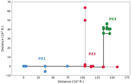
Figure 1.
IEEE 34 nodes system divided in 3 PZs: PZ1 (blue), PZ2 (red) and PZ3 (green).
- PZ1: 800, 802, 806, 808, 810, and 812.
- PZ2: 814, 850, 816, 824, 826, 828, 830, 854, 856, 818, 820, and 822.
- PZ3: 852, 832, 888, 890, 858, 864, 834, 842, 844, 846, 848, 860, 836, 840, 862, and 838.
It is important to note that every node carries a GCN model, and is able to detect and locate faults. The faults are simulated in all nodes except in the substation (Node 800). The fault simulation parameters depend on the number of phases in the node. For 3P nodes, the parameter combinations are shown in Table 1.

Table 1.
Fault parameters for 3P nodes.
This sums up a total of 66 faults per 3P node. For 1P nodes, in order to increase the number of fault simulations and balance out the existence of just one type of fault, additional combinations of inception angles and resistance values are considered. The combinations for 1P nodes use the following parameters, as shown in Table 2.
Table 2.
Fault parameters for 1P nodes.
Therefore, there are a total of 48 fault cases for each 1P node. Among the fault cases, 80% were employed to train the GCN models, while the other 20% were used for testing. Taking into account all the nodes in each PZ, the total number of simulations in each zone can be observed in Table 3. Note that the GCN models are trained with 10-fold cross-validation. This means that the models are trained 10 times, and that in each run, one-tenth of the faults are used as a validation dataset in which the models’ performance is tested for each epoch. A learning rate scheduler is set to decrease the learning using a factor of 0.9 if the validation score does not improve in four consecutive epochs.
Table 3.
Number of faults per PZ.
5. The Method
In each node, either 3P or 1P voltage, current, or both, measurements are recorded at a sampling rate of 1 MHz. The DMD algorithm, as described in [28], is used to pinpoint the TW arrival time at each node. This algorithm is selected because of its sensitivity, as training the GCN models requires that all nodes detect the fault in order to have some initial features. Then, the measurements undergo a time–frequency decomposition that extracts the high-frequency components in the signals. Eventually, these features are fed into the GCN models for fault protection zone classification. There are four GCN model versions in which the models’ size and the employed type of measurements (either voltage, current, or both) vary for a sensitivity analysis.
5.1. Signal Processing Stage
The signal processing stage design is critical for the success of this implementation. It has to provide sufficiently detailed feature extraction/creation, but it has to be light enough so that the microcontroller can execute it in a reasonable amount of time while observing the device’s memory constraints. Similarly, the number of sample points that are processed at a single step also has to be small so it can be managed by the microcontroller. After successful detection, the measurements are cropped −32/+96 samples around the TW arrival timestamp for each phase and type of measurement. The samples’ array length is 128 values, which corresponds to 128 microseconds (μs). This choice of signal length is related to the consecutive halving that takes place in the DWT decomposition, which makes it more desirable to work with signal lengths that are a power of 2 (note that ). For this work, the input to the microcontroller is the set of 3P/1P (depending on the node type) voltage, current, or both, with measurement arrays (depending on the GCN model to be implemented) of 128 values each.
Afterwards, the signal processing stage to be executed in the microcontroller is divided into three consecutive steps: The Karrenbauer transformation (KT) for the 3P nodes; the DWT decomposition; and the Parseval’s energy (PE) theorem. All four models share the same signal processing stage. The only difference is the size of the output values in each step (detailed below) and the tentative execution time (if both the voltage and current measurements are used, the signal-processing stage is conducted twice).
5.1.1. The Karrenbauer Transformation
The KT is commonly used for decomposing a 3P signal into decoupled modes. The ground mode is very sensitive to attenuation due to distance [36], so it is preferred for ML/DL approaches as it incorporates additional information about the distance to the fault. In this work, due to the fact that the same amount of information has to be employed by every node, 3P nodes have their voltage and current measurements summarized in the ground mode. For 1P nodes, the KT is not applied and the available phase measurements are employed directly. In Equation (1), the ground mode for voltage is calculated as follows considering that , and are the 3P voltage measurements.
If both the voltage and current measurements are considered, the output of the KT is two arrays of length 128 samples each: a ground mode for voltage and one for current. For the models in which only one magnitude is considered, the output is an array of 128 samples.
5.1.2. The Discrete Wavelet Transform
The DWT is a very common tool for time–frequency decomposition. It is faster to execute than the CWT, while it is less resource expensive than other discrete WT such as the stationary wavelet transform (SWT). This last statement is based on the fact that the DWT halves signals’ length in each decomposition level, while the SWT exponentially upsamples the filter length at every level [37]. Therefore, the DWT is more suitable for memory-sensitive applications.
The DWT is efficiently implemented using multi-resolution analysis (MRA) [38]. MRA consists of using a combination of half-band low-pass (LP) and high-pass (HP) filters in order to decompose a signal into frequency bands. The output of the HP filter is called “detail” decomposition coefficients, while the output of the LP filter is called “approximation” decomposition coefficients. The detail coefficients summarize the signal’s frequency components of the upper-half of the frequency spectrum for each particular level of decomposition, while the approximation coefficients summarize the lower-half band. The approximation coefficients are then fed into the next decomposition level for further decomposition. The workflow of this process can be appreciated in Figure 2. The HP and LP filter coefficients are the same for every level. The coefficients are extracted from the Daubechies 4 (db4) mother wavelet, used in this work. The db4 is an 8th order filter. This wavelet family is particularly suitable for TW applications because their sharp shape is perfect for detecting a low amplitude, short duration, and fast decay signals [39]. In the end, only the detail coefficients are employed to characterize a signal’s decomposition into frequency bands, as these bands are clearly delimited. For a three-level DWT decomposition, the frequency bands for the detail coefficients can be observed in Table 4. It is important to note that, as in consecutive decomposition levels, the maximum frequency to be measured is halved, the sampling frequency can be halved as well without loss of information according to the Nyquist Theorem. In the DWT, it means that at every decomposition level the detail and approximation coefficients are downsampled by a rate of 2.
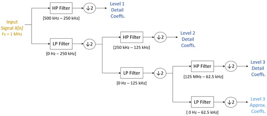
Figure 2.
Workflow of the DWT decomposition in 3 levels.
Table 4.
Frequency bands for DWT decomposition in 3 levels.
For implementation in the microcontroller, there are two basic operations that are required to execute a DWT decomposition:
- A convolution between the LP/HP filter coefficients and the input signal or the approximation coefficients from the previous level. The FIR filter functions in the FPU library offer a method to perform convolutions very efficiently, reducing the need for two loops to just one. It is important to note that this convolution operation assumes that the input is zero-padded.
- A downsampling operation, in which only the odd output coefficients are retained.
The detail coefficients of all levels are later reconstructed to obtain 128-values volts and amperes signals (which complete the time–frequency signal decomposition into frequency bands). This is achieved by following the inverse process, using the synthesis filters instead of the decomposition counterparts, and upsampling instead of downsampling. For the reconstruction of each single array of detail coefficients, every other array is filled up with zeros so they do not intervene in the reconstruction process. Optimizing the number of decomposition levels against the execution time, it was determined that the signal decomposition was in three levels, and the following reconstruction can be successfully implemented in less than 1 ms (as it is detailed in the results section). This is a proper signal processing stage execution time targeting a TW-based protection implementation.
Due to this implementation of the filter convolutions, there are some undesirable “edge effects” at the beginning and end of the signal which are caused by the fact that not all of the filter coefficients are part of the convolution in the first and last signal values. Thereby, this causes some artifacts to not be part of the TW, but of the convolution implementation itself. Therefore, the 128 values of the reconstructed signals are cropped again, removing the first and last 32 samples. This leaves the TW arrival in the first sample and removes any undesirable artifacts. For the models in which both voltage and current are employed, the output of the DWT decomposition and reconstruction is a set of six arrays of a length of 64 values each (three levels for voltage and three levels for current). For the models in which only voltage or current is used, the output of this stage is 3 arrays of 64 values each.
5.1.3. Parseval’s Energy Theorem
The PE theorem is employed in this work to create non-decreasing arrays in which the magnitude of the TW reflections are amplified. The PE theorem is computed using the following expression for each of the arrays:
Finally, all the PE levels are concatenated into a single array of size 384, if both voltage and current are employed, or 192 otherwise if just one of the measurement types is considered. The result of this step is downsampled by 2 to decrease the size of the inputs for the GCN models, which translates into huge savings in used memory. Therefore, the output of the signal-processing stage is an array of 192 values if both voltage and current measurements are employed, or 96 values if only one of the measurement types is employed.
As a summary of the signal-processing stage, the input and output of each step depend on the node type and the number of measurements of voltage, current, or both, as detailed in Figure 3.
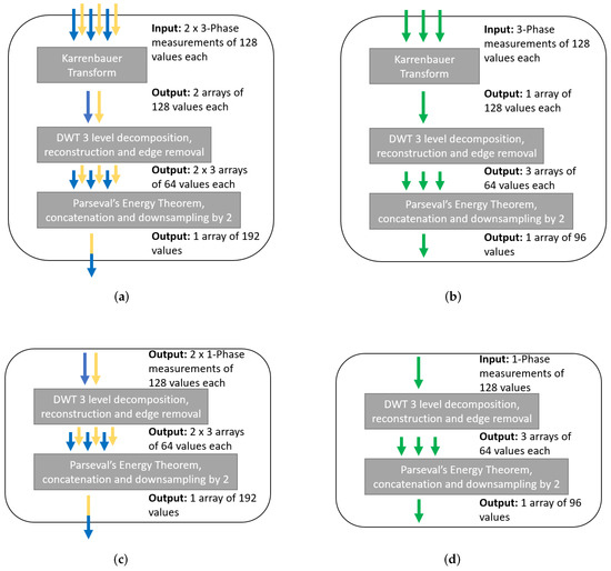
Figure 3.
Signal processing stage per node type and type of measurements: (a) 3P node, V and I; (b) 3P node, either V or I; (c) 1P node, V and I; and (d) 1P node, either V or I.
5.2. Protection Zone Prediction Stage
5.2.1. Introduction to Graph Neural Networks
GCNs are especially beneficial to power systems as they provide a spatial relationship to the voltage and current measurements. In each layer, GCNs aggregate the information of neighboring nodes to update the nodes’ status. This is known as a message-passing network. The connection between nodes is modeled using the adjacency matrix A [40], which in this work is binary: if two nodes i and j are neighbors, the element of the matrix is equal to 1, or it is 0 otherwise. The initial node data are gathered in a feature matrix X, whose size is , where n is the number of nodes in the system and d is the length of the feature vector per node. A GCN model has the following layer-wise propagation rule [41]:
where is the modified adjacency matrix A considering the self-connections adding the identity matrix I, is the optional layer-specific trainable bias term, is the layer-specific trainable weight matrix, is the activation function, and D is the diagonal node degree matrix of the adjacency matrix , which is defined as:
and is the output of the layer. Note that in the first layer. If edges are weighted, the formula is modified to:
where is the output of the layer for node i, is the product of the square root of node degrees, and is the scalar weight on the edge from node j to node i. In this work, is the distance between nodes in feet. Note that both and are the same for all the nodes. Finally, the edge weights can be normalized by applying the following expression:
5.2.2. GCN Models
There are four versions of GCN models attending to the weight matrices’ size and which measurements (either voltage, current, or both) are used as inputs. Nevertheless, all models consider the same signal-processing stage and all of them have three GCN layers. The output of the last GCN layer has the same size as the number of PZ, which is three. The output goes through a Log-Softmax layer that returns the log-probabilities that the fault is in each PZ. There are two models that use both current and voltage. One has larger weight matrices (“Heavy VI”), while in the other one, the number of weights is comparatively smaller (“Light VI”). Then, there is another that uses only voltage measurements (“Only V”), and another one that only uses current measurements (“Only I”). The layer’s input size for each model is summarized in Table 5. The aim is to analyze the sensitivity of the models’ size and measurements’ type against the models’ accuracy. Models are trained in Pytorch using Deep Graph Library [42].
Table 5.
Layers’ size for each GCN model.
5.2.3. Distributed Implementation
The GCN model implementation to be executed in each corresponding node is identical for the four versions, and utilizes the same expressions as in Equations (5) and (6). In order to try this on an experimental implementation in a microcontroller, node 828 is used as an example. This node is connected to nodes 824 and 830. These are the elements to be considered for a given layer l:
- The bias term and the weights , which are shared with all the other nodes in the system.
- The incoming messages are from neighboring nodes 824 and 830, and . These are the outputs from the previous layer in those nodes. For , they are the output of the signal processing stage.
- The output from the previous layer , which is the input of the current layer.
- The normalized edge weights for message-passing from node 824 to node 828 and from node 830 to node 828, and , and the self-loop for node 828, .
As an example, the workflow for layer can be observed in Figure 4.
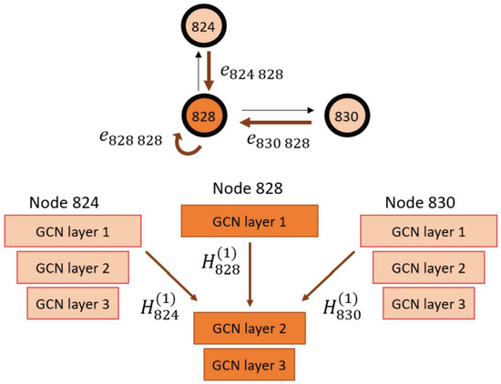
Figure 4.
Message-passing for GCN L=layer 2 at node 828.
6. Experimental Setup
In order to test the computation time of the proposed method, a TW fault testing bench was designed. This experimental setup allows for the playback of simulated fault signals at 1 MHz. Note that a detection stage has to be introduced prior to the fault location algorithm. In this work, we incorporate a DWT-based TW detection that was previously introduced in [43], and experimentally validated in [44]. This detection method provides a reliable and fast detection method, taking approximately 128 microseconds to execute the algorithm. A brief introduction to the method is provided in Section 6.1.
6.1. Experimental TW Detection
The employed TW detection method is based on the DWT. The method is implemented on a per-phase basis, which is due to the computation limitations of the microcontroller. Hereafter, the computations that are carried out for a single-phase are described. A high-level workflow of the method is shown in Figure 5. The CLA continuously samples the voltage signal at 1 MHz, and the values are stored in a circular buffer of length 128. When the buffer is full, this array of 128 values is passed to the CPU. Then, the first DWT level of decomposition is executed to retrieve the first detail coefficients. As can be appreciated in Table 4, these coefficients summarize the frequency components in the range from 250 kHz to 500 kHz. Then, the maximum absolute value of such coefficients is extracted and compared to a pre-defined threshold. In [43], it is explained how this threshold can be obtained. In practice, a threshold that is right above the values produced by measuring noise in normal operation is enough for detection purposes in an experimental setting. Once a TW event has been detected, the same logic is executed again, but this time looping through the absolute value of all coefficients, to find the first detail coefficient which is above the threshold. The TW arrival time is the index of such a coefficient. The final output of the detection process is the cropped signal in the −32/+96 samples around the TW arrival timestamp. This may require waiting until the next period of 128 samples. More information about the process and the execution times can be found in [44]. Note that the analysis of a signal has to take less than 128 μs to make the method feasible.
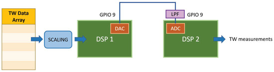
Figure 5.
Experimental setup for fault detection testing.
6.2. TWs Fault Bench
The fault testing experimental setup is composed of just two microcontrollers. The first one, also called the “sender”, is in charge of the playback function. The second microcontroller, the “receiver”, is constantly sampling for an incoming TW. Due to the computation limitations—there is not enough computational speed to analyze three signals in a period of 128 μs- the receiver only covers one-phase at a time. In order to capture the TW in the three-phases, the playback is repeated three times, varying the signal that is reproduced. A schematic of the fault bench can be observed in Figure 5. The TW data come from the PSCAD simulations. Both devices use the GPIO pin 9, that can be configured as an ADC or an DAC. The receiver incorporates an analog anti-aliasing first-order low-pass filter that removes any high-frequency noise that goes beyond the analyzed frequency components. The cut-off frequency is 600 kHz. The usage of just two development boards constitutes a low-cost testing environment. It would be possible to use three devices, one per-phase, to do a simultaneous TW detection. However, given that operating a development board requires a computer, this option would require a total of four computers.
For the TW playback, a 3P voltage waveform of a 2 ms duration was loaded onto the sender’s look-up table in the form of a one-dimensional array. The original data are in units of kV, but it has to be linearly scaled using the expression in:
to adapt the values to the dynamic range of the ADC, which is from 0 to = 4096. Note that is the array to be loaded onto the DAC, and the is the simulated data, which for the example that is used in this work is comprised in the range of [−21, 21] kV. The entire length of the signal is reproduced at 1 MHz by the sender microcontroller, while the receiver microcontroller on the other end samples the incoming signal at 1 MHz.
7. Results
7.1. Models’ Accuracy Comparison
These results are for simulated data. The nodes’ accuracy distributions are depicted in Figure 6. No measurement noise was considered. The median accuracy value is displayed as a red vertical line in each of the plots. Some statistical quantities of such distributions are gathered in Table 6. The Heavy VI shows the strongest performance, with the largest median accuracy and overall accuracies (one-half of the nodes are above 87% accuracy). It is followed by the Only V model, which has a lower maximum node accuracy, but also a higher minimum node accuracy. The Light VI shows a few really large accuracy values, but most of the nodes’ accuracies are located in a broad distribution between 70% and 90%, which is not desirable. Finally, the Only I has a poor performance in comparison to other models, although it achieves the maximum node accuracy, a 94.85%.
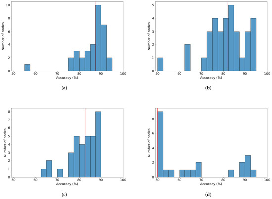
Figure 6.
Nodes’ accuracy histograms for GCN models: (a) Heavy VI; (b) Light VI; (c) Only V; and (d) Only I.
Table 6.
Testing accuracy analysis per model.
Figure 7 shows the nodes’ accuracy for each model. Each diagram shows the 3P lines colored in black, while 1P lines are plotted in gray. As can be seen, the overall nodes’ accuracy is good in the Heavy VI, Light VI, and Only V models, and most of the weaker performing nodes are on laterals. The Heavy VI model’s overall performance is slightly better than the Light VI and Only V models, as expected.
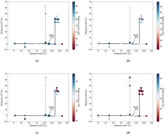
Figure 7.
Nodes’ individual accuracy for GCN models: (a) Heavy VI; (b) Light VI (c) Only V; and (d) Only I.
7.2. Models’ Resiliency to Communication Losses
Node 828, which is located near the center of the system as can be seen in Figure 7, performs well with both Heavy VI and Only V models. Therefore, this node is selected to analyze the resiliency of the proposed protection scheme for communication losses. Note that the results in this section are obtained with simulated data in PSCAD, not experimentally measured data. The fact that the GCN models are a distributed approach, and that messages between nodes are required to come up with a prediction, make the proposed fault location method sensitive to communication failures or cyber-attacks. However, it is important to highlight that distributed approaches are generally more resilient to unexpected events than centralized ones [45]. In order to check the models’ resiliency, several scenarios in which messages do not arrive on time (and thereby substituted by arrays of zeroes) are analyzed. As mentioned before, the GCN models are implemented in node 828, which is connected to nodes 824 and 830. As there are three GCN layers and two neighbors, a total of six messages are expected. These are the communication loss cases in which the resiliency of the models is tested:
- Case A: There is no failure in communication and it is used as the baseline.
- Case B and C: One neighbor is not available and no messages are received. Then, 3 messages are lost.
- Cases D–I: One message, in one of the layers, and from either of the neighbors, is lost.
- Cases J–O: Two messages, in different layers, and from either of the neighbors, are lost.
- Cases P–U: Three messages, in different layers and from different nodes, are lost.
A more detailed description of each case is provided in Table A1 in Appendix A. The accuracy results of these cases are gathered in Table 7, Table 8, Table 9 and Table 10.
Table 7.
Testing accuracy analysis per model for cases A–C.
Table 8.
Testing accuracy analysis per model for cases D–I.
Table 9.
Testing accuracy analysis per model for cases J–O.
Table 10.
Testing accuracy analysis per model for cases P–U.
The accuracy upper-bound is given by case A, in which there are no communication issues. Some cases produce a drop in accuracy. Typically, the more severe the scenario is, the higher the chance (and the magnitude) of a drop in accuracy. However, the accuracy drops are bounded (the worst cases are observed in the “Heavy VI” model in which the accuracy drops 17.9%). Taking into account the small size of the models, they perform relatively well to significant communication failures.
7.3. Models’ Execution Time Comparison
For the experimental validation of the method’s computing requirements, node 828 is emulated in the F28379D microcontroller. For this section, both the fault detection and computation times are considered. The fault detection part is considered as a black-box stage, as a more detailed analysis can be found in [44]. According to the previously explained detection method, the TW detection is carried out first, one phase at a time, and the obtained TWs are saved. Afterward, the three detected TWs, without any modifications, are the input to the location process. As of now, it is not a standalone process, but both stages are consecutive and perfectly connected. That is why the combination of both detection and location execution times can be jointly considered to provide an accurate estimation of the total execution time.
In this work, the performance of the model for a specific fault case was tested. The fault data are as follows: The fault type is 3P, the fault location is node 806 (PZ1), and the fault impedance is 0.01 . As mentioned before, the fault detection method is executed independently on a per-phase basis. The results of the fault detection stage are shown in Figure 8. All signals are cropped in the −32/+96 samples fashion around the detected TW arrival timestamp. As can be noticed, the match between the simulated and measured signal by the receiver microcontroller is very good. There are some minor issues, such as some distortion, and some offset by being inherently introduced by the DAC and the ADC. In addition, the TW detection in phase A has a small shift of two samples.
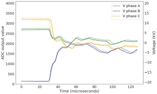
Figure 8.
TW experimental fault detection comparison between the original waveform to be reproduced by the sender (dashed) and the measured waveform by the receiver (solid).
The Only V model is coded into the microcontroller given that the signal processing stage only has to be carried out once (for voltage). This process uses the bias term and the weights of the trained models, and replicates the equation in Equation (7) in the C programming language. Note that the communication protocols for message-passing between nodes are not in the scope of the project. However, the communication delay can be expected to be just tens of microseconds if technologies such as fiber-optic are used. State-of-the-art fiber-optic latency is approximately 5 microseconds per kilometer [46], which is several orders of magnitude smaller than the execution time of the proposed algorithms.
The fault location method that is proposed in this paper is implemented into the microcontroller in three distinct stages:
- Pre-processing: Once the three arrays of 128 values are retrieved by the detection stage, the first step is to scale them back to kV and to calculate the ground mode, which is the only decoupled mode that is used in this work. Both operations are efficiently executed at the same time using the following expression:
- Feature extraction: The voltage ground mode undergoes a three-level DWT decomposition and reconstruction that retrieves a total of three arrays of 128 values each, summarizing the signal’s frequency components in the frequency bands, as observed in Table 4. Note that just 64 samples per array are retained, starting on the detected TW arrival timestamp. Afterwards, the PE values of such arrays are calculated and concatenated, forming a single array of features containing 192 values. To fit the model’s input layer, further downsampling by 2 is conducted to retrieve the final array of 96 samples.
- GCN model: The implemented fault location model is the Only V model, as previously defined in Table 5. There are RELU non-linear activation functions after the two first GCN layers, while the final layer is a Log-Softmax layer that retrieves the log-probabilities of the fault being in each of the three considered PZs. Incoming communication from nodes 824 and 830 is required in each GCN layer. The messages are previously loaded into the microcontroller and not considered in the execution time, as the communication delay is much smaller than the actual execution time.
A workflow of the previously described implementation can be seen in Figure 9.
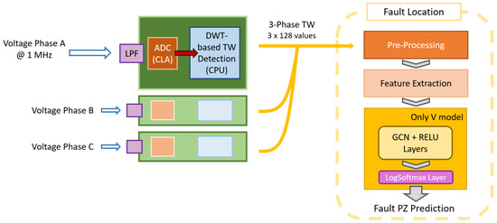
Figure 9.
Workflow of the fault detection and location methods in the microcontroller.
Regarding the accuracy performance of the implementation in the microcontroller, which includes real sampling of a TW at 1 MHz, the method accurately locates the fault in PZ1. The output of the model, the Log-Softmax layer, returns the log-probabilities of the fault being in each of the three PZs. The comparison between the log-probabilities obtained in the experiment and the ones obtained from the simulated data are shown in Table 11. For an easier comparison, the exponential of base e is used to retrieve the percentages.
Table 11.
Faulty PZ predictions between the simulated model and the experimental test.
In Table 12, a summary of the execution time of the proposed method is attached. The TW detection stage executes in approximately 150 μs [44], including the saving of the cropped signal into a variable. No significant differences can be pointed out in the execution time per-phase. The location stage starts from this same point, and executes the three previously described stages. The signal processing stage is by far the most computationally expensive, which takes more than 800 μs. Adding the execution times of both fault detection and location stages, the proposed method requires an estimated total of 1.27 milliseconds to execute.
Table 12.
Summary of stages’ execution times.
For a more thorough analysis of the fault location method, a detailed breakdown is provided in Table 13. The ground mode and de-scaling are executed in a single loop using the expression in (9), and constitute the longest single calculation in the method. Regarding the feature extraction stage, it can be noticed that the decomposition becomes faster as the decomposition level increases. This is because the consecutive halving of the signal makes the further convolutions shorter. However, for the reconstruction, the larger the decomposition level, the more time it takes to calculate the required convolutions back. Up to level 3, it can be noticed that each level takes a joint time of 50 × 103 CPU cycles (250 μs), combining both decomposition and reconstruction. Afterward, the calculation and further downsampling of the PE values are relatively faster. Finally, the execution of the GCN model is the fastest stage. The first GCN layer takes significantly more time than the other two because the number of parameters is much larger, as can be seen in Table 5. Non-linear activation layers are executed extremely quickly.
Table 13.
Detailed breakdown of the fault location execution times.
Regarding the memory allocation of the model in the microcontroller, Table 14 details the text file size, which is the size of the .h file in the computer file explorer, and the reported allocated memory in the microcontroller, including both the used space for the variables and the raw data. The superscript indicates the corresponding GCN layer. Note that the number of bytes is significantly lower on the compiled code. The total size of the model is 22.8 kB, which is approximately one-third of the available globally shared memory (64 kB). If necessary, there are other smaller local memory registers that could be used as well.
Table 14.
Memory allocation of the model’s weights and bias terms.
8. Discussion
The contribution of this paper is very significant for distribution power system protection. To the best of our knowledge, this is the first implementation of a fault location method that jointly employs TWs and a DL model (in this case, a novel GCN model that can be coded into a microcontroller). More importantly, this work also details the execution time of the method, which is in line with other TW protection devices for transmission systems (but that do not use any type of ML or DL models) [16].
This work is interpreted as a demonstration of the feasibility of DL models for ultra-fast protection in distribution systems, paving the way for a future commercial application. The reality is that the models that are evaluated in this work are just scaled-down versions of the models that have been previously researched in [31]. This is because of the memory and computation constraints of the employed development board (which has one of the fastest microcontrollers that are available today). For the same reason, detection and location methods have to be executed separately and not as a standalone method. However, it can be expected that, given the right embedded device is employed, full-scale and high-accurate methods can be deployed and executed in a matter of hundreds of microseconds. Furthermore, the developed fault bench using two development boards is a simple but reliable way of testing TW protection schemes in microcontrollers, reproducing waveforms that are generated in simulations with complex power networks at speeds of 1 MHz.
Finally, GCN models are a promising implementation of ML/DL-based protection relays. The fact that all nodes in the system carry the same model facilitates its training, which takes into account all nodes at the same time, and its later deployment in the field. For more complex systems, the method could be generalized by dividing the power grid into several sub-graphs, allowing for either training local models, or including different systems as part of the same training batch to create a global model.
9. Conclusions
This work proposes a set of scaled-down graph convolutional network (GCN) models for fault location in the IEEE 34-node system. The goal is to determine in which protection zone (PZ) the fault occurred. The system is divided into three PZs. One of these models was later implemented into a microcontroller to measure the execution time of the algorithm.
The method uses only 128 microseconds of fault traveling wave (TW) data. A feature extraction stage was designed including the following steps: firstly, the Karrenbauer transform (KT) is performed to calculate the ground mode of the three-phase (3P) nodes. For one-phase (1P) nodes, measurements are used directly. Then, a time–frequency decomposition of the signals is conducted using the discrete wavelet transform (DWT). This method is focused on frequency-components between 62.5 and 500 kHz. Finally, the Parseval energy (PE) of the decomposed signals is calculated, and these features are used to train the GCN models. Models are trained using just the first 64 microseconds of the PE values, which is shown to achieve good performance while reducing the usage of memory.
A total of four GCN models were trained, using either voltage, current measurements or both. For both measurements, two models of different sizes were created. All models have three GCN layers. The models that use both voltage and current, or just voltage, achieve median node accuracies in the range of 80–90%, which is a good performance taking into account the memory and time constraints under which the method was designed. The performance of the model that only uses the current measurement is significantly lower. Node 828 is considered a role-model node in the system, as it performs well under several models. This node is chosen to conduct a resiliency analysis for communication losses, and later the microcontroller implementation. Regarding the resiliency analysis, 20 different cases are considered in which between 1 and 3 messages from different communication channels are dropped. Compared to the baseline, lost messages could decrease the node-wise accuracy from 15% to 20%. A decrease in accuracy is more probable for a larger loss of information.
Regarding the implementation in the microcontroller, the model that only uses voltage measurements is coded in the C language. The model weights use up to one-third of the available global memory. An experimental fault bench is created connecting two microcontrollers. This way, one device can reproduce a TW while the second can sample it at 1 MHz. One particular fault case in the first PZ is tested. The TW is detected using a DWT-based approach that is used per-phase. It takes approximately 0.15 milliseconds to detect the TW and store the data. The resulting measurements are then fed into the proposed fault location algorithm, which is executed in approximately 1.12 milliseconds. The measurement noise and distortion do not significantly affect the overall performance of the method, which retrieves the same output probabilities compared to the simulated case. The total estimated execution time of this method is 1.27 milliseconds, which is in line with other TW protection schemes at the transmission level, but they do not use machine or deep learning models.
Author Contributions
Conceptualization, M.J.-A.; methodology, M.J.-A.; software, M.J.-A., J.H.-A. and A.Y.M.; validation, M.J.-A., J.H.-A., A.Y.M. and M.J.R.; formal analysis, M.J.-A.; investigation, M.J.-A. and J.H.-A.; resources, M.J.-A.; data curation, M.J.-A.; writing—original draft preparation, M.J.-A.; writing—review and editing, M.J.-A., J.H.-A., A.Y.M. and M.J.R.; visualization, M.J.-A.; supervision, M.J.R. All authors have read and agreed to the published version of the manuscript.
Funding
This material was based upon work supported by the Laboratory Directed Research and Development program at Sandia National Laboratories and the U.S. Department of Energy’s Office of Energy Efficiency and Renewable Energy (EERE) under Solar Energy Technologies Office (SETO) Agreement Number 36533. Sandia National Laboratories is a multimission laboratory managed and operated by National Technology and Engineering Solutions of Sandia, LLC, a wholly owned subsidiary of Honeywell International, Inc., for the U.S. Department of Energy’s National Nuclear Security Administration under contract DE-NA0003525. This paper describes objective technical results and analysis. Any subjective views or opinions that might be expressed in the paper do not necessarily represent the views of the U.S. Department of Energy or the United States Government.
Data Availability Statement
The data presented in this study are available upon request from the corresponding author. The data are not publicly available due to the data privacy policy of the funding entities.
Conflicts of Interest
The authors declare no conflict of interest.
Abbreviations
The following abbreviations are used in this manuscript:
| TW | Traveling Wave |
| SWT | Stationary Wavelet Transform |
| CWT | Continuous Wavelet Transform |
| DWT | Discrete Wavelet Transform |
| MRA | Multi-Resolution Analysis |
| LP | Low Pass |
| HP | High Pass |
| KT | Karrenbauer Transform |
| PE | Parseval’s Energy |
| DMD | Dynamic Mode Decomposition |
| GNN | Graph Neural Network |
| GCN | Graph Convolutional Network |
| AI | Artificial Intelligence |
| ML | Machine Learning |
| DL | Deep Learning |
| SLG | Single Line to Ground |
| LL | Line to Line |
| 1P | One Phase |
| 3P | Three Phase |
| LLG | Line to Line to Ground |
| 3PG | Three Phase to Ground |
| PZ | Protection Zone |
| CLA | Control-Law Accelerator |
| CPU | Central Processing Unit |
| FPU | Floating-Point Unit |
| ADC | Analog-to-Digital Converter |
| DAC | Digital-to-Analog Converter |
Appendix A
Table A1.
Received message from neighbors in node 828, per GCN layer, for each case in the communication losses study.
Table A1.
Received message from neighbors in node 828, per GCN layer, for each case in the communication losses study.
| Case | ||||||
|---|---|---|---|---|---|---|
| A | ✓ | ✓ | ✓ | ✓ | ✓ | ✓ |
| B | ✓ | X | ✓ | X | ✓ | X |
| C | X | ✓ | X | ✓ | X | ✓ |
| D | X | ✓ | ✓ | ✓ | ✓ | ✓ |
| E | ✓ | X | ✓ | ✓ | ✓ | ✓ |
| F | ✓ | ✓ | X | ✓ | ✓ | ✓ |
| G | ✓ | ✓ | ✓ | X | ✓ | ✓ |
| H | ✓ | ✓ | ✓ | ✓ | X | ✓ |
| I | ✓ | ✓ | ✓ | ✓ | ✓ | X |
| J | ✓ | ✓ | X | ✓ | ✓ | X |
| K | ✓ | X | X | ✓ | ✓ | ✓ |
| L | X | ✓ | ✓ | ✓ | ✓ | X |
| M | ✓ | X | ✓ | ✓ | X | ✓ |
| N | ✓ | ✓ | ✓ | X | X | ✓ |
| O | X | ✓ | ✓ | X | ✓ | ✓ |
| P | X | ✓ | X | ✓ | ✓ | X |
| Q | ✓ | X | ✓ | X | X | ✓ |
| R | X | ✓ | ✓ | X | ✓ | X |
| S | ✓ | X | X | ✓ | X | ✓ |
| T | X | ✓ | ✓ | X | X | ✓ |
| U | ✓ | X | X | ✓ | ✓ | X |
Note: The subscript indicates the GCN layer in which the message takes place.
References
- U.S. Department of Energy. Internet of Things-Enabled Devices and the Grid; U.S. Department of Energy: Washington, DC, USA, 2017.
- Meliopoulos, A.P.S.; Cokkinides, G.J.; Huang, R.; Polymeneas, E.; Myrda, P. Grid Modernization: Seamless Integration of Protection, Optimization and Control. In Proceedings of the 2014 47th Hawaii International Conference on System Sciences, Waikoloa, HI, USA, 6–9 January 2014; pp. 2463–2474. [Google Scholar] [CrossRef]
- Velaga, Y.N.; Prabakar, K.; Singh, A.; Sen, P.K.; Kroposki, B.D. Advanced Distribution Protection for High Penetration of Distributed Energy Resources (DER); National Renewable Energy Lab. (NREL): Golden, CO, USA, 2019.
- Guzmán, A.; Kasztenny, B.; Tong, Y.; Mynam, M.V. Accurate and economical traveling-wave fault locating without communications. In Proceedings of the 2018 71st Annual Conference for Protective Relay Engineers (CPRE), College Station, TX, USA, 26–29 March 2018; pp. 1–18. [Google Scholar] [CrossRef]
- IEEE Std C37.114-2014 (Revision of IEEE Std C37.114-2004); IEEE Guide for Determining Fault Location on AC Transmission and Distribution Lines. IEEE: Manhattan, NY, USA, 2015; pp. 1–76. [CrossRef]
- Wilches-Bernal, F.; Bidram, A.; Reno, M.J.; Hernandez-Alvidrez, J.; Barba, P.; Reimer, B.; Montoya, R.; Carr, C.; Lavrova, O. A Survey of Traveling Wave Protection Schemes in Electric Power Systems. IEEE Access 2021, 9, 72949–72969. [Google Scholar] [CrossRef]
- Jahromi, A.T.; Wolfs, P.; Islam, S. A travelling wave detector based fault location device and data recorder for medium voltage distribution systems. In Proceedings of the 2016 Australasian Universities Power Engineering Conference (AUPEC), Brisbane, QLD, Australia, 25–28 September 2016; pp. 1–5. [Google Scholar] [CrossRef]
- Bewley, L.V. Traveling waves on electric power systems. Bull. Am. Math. Soc. 1942, 48, 527–538. [Google Scholar] [CrossRef]
- Greenwood, A. Electrical Transients in Power Systems, 2nd ed.; Wiley-Interscience: New York, NY, USA, 1991. [Google Scholar]
- Barnett, P.S. The Analysis of Travelling Waves on Power System Transmission Lines. Ph.D. Thesis, University of Canterbury, Electrical Engineering, Christchurch, New Zealand, 1974. [Google Scholar]
- Benato, R.; Sessa, S.D.; Poli, M.; Quaciari, C.; Rinzo, G. An Online Travelling Wave Fault Location Method for Unearthed-Operated High-Voltage Overhead Line Grids. IEEE Trans. Power Deliv. 2018, 33, 2776–2785. [Google Scholar] [CrossRef]
- Lopes, F.V.; Dantas, K.M.; Silva, K.M.; Costa, F.B. Accurate Two-Terminal Transmission Line Fault Location Using Traveling Waves. IEEE Trans. Power Deliv. 2018, 33, 873–880. [Google Scholar] [CrossRef]
- Jin, W.; Lu, Y.; Tang, C. A novel double ended method for fault location based on travelling wave time-series. In Proceedings of the 2016 IEEE International Conference on Power System Technology (POWERCON), Wollongong, NSW, Australia, 28 September–1 October 2016; pp. 1–6. [Google Scholar] [CrossRef]
- Schweitzer, E.O.; Guzmán, A.; Mynam, M.V.; Skendzic, V.; Kasztenny, B.; Marx, S. Locating faults by the traveling waves they launch. In Proceedings of the 2014 67th Annual Conference for Protective Relay Engineers, College Station, TX, USA, 31 March–3 April 2014. [Google Scholar] [CrossRef]
- Guzmán, A.; Mynam, V.; Mangapathirao Skendzic, V.; Eternod, J.L. Directional Elements—How Fast Can They Be? In Proceedings of the 44th Annual Western Protective Relay Conference, Spokane, WA, USA, 17–19 October 2017. [Google Scholar]
- Schweitzer, E.O.; Kasztenny, B.; Mynam, M.V. Performance of time-domain line protection elements on real-world faults. In Proceedings of the 2016 69th Annual Conference for Protective Relay Engineers (CPRE), College Station, TX, USA, 4–7 April 2016. [Google Scholar] [CrossRef]
- Lout, K.; Aggarwal, R.K. A feedforward Artificial Neural Network approach to fault classification and location on a 132kV transmission line using current signals only. In Proceedings of the 2012 47th International Universities Power Engineering Conference (UPEC), Uxbridge, UK, 4–7 September 2012; pp. 1–6. [Google Scholar] [CrossRef]
- Yadav, A.; Swetapadma, A. Combined DWT and Naive Bayes based fault classifier for protection of double circuit transmission line. In Proceedings of the International Conference on Recent Advances and Innovations in Engineering (ICRAIE-2014), Jaipur, India, 9–11 May 2014; pp. 1–6. [Google Scholar] [CrossRef]
- Sun, J.; Wen, X.; Wei, X.; Chen, Q.; Wang, Y. Traveling Wave Fault Location for Power Cables Based on Wavelet Transform. In Proceedings of the 2007 International Conference on Mechatronics and Automation, Harbin, China, 5–8 August 2007; pp. 1283–1287. [Google Scholar] [CrossRef]
- Borghetti, A.; Bosetti, M.; Silvestro, M.D.; Nucci, C.A.; Paolone, M. Continuous-Wavelet Transform for Fault Location in Distribution Power Networks: Definition of Mother Wavelets Inferred From Fault Originated Transients. IEEE Trans. Power Syst. 2008, 23, 380–388. [Google Scholar] [CrossRef]
- Borghetti, A.; Bosetti, M.; Nucci, C.A.; Paolone, M.; Abur, A. Integrated Use of Time-Frequency Wavelet Decompositions for Fault Location in Distribution Networks: Theory and Experimental Validation. IEEE Trans. Power Deliv. 2010, 25, 3139–3146. [Google Scholar] [CrossRef]
- Chen, X.; Yin, X.; Yin, X.; Tang, J.; Wen, M. A novel traveling wave based fault location scheme for power distribution grids with distributed generations. In Proceedings of the 2015 IEEE Power & Energy Society General Meeting, Denver, CO, USA, 26–30 July 2015; pp. 1–5. [Google Scholar] [CrossRef]
- Jimenez Aparicio, M.; Grijalva, S.; Reno, M.J. Fast Fault Location Method for a Distribution System with High Penetration of PV. In Proceedings of the 54th Hawaii International Conference on System Sciences, Kauai, HI, USA, 5–8 January 2021. [Google Scholar] [CrossRef]
- Jiménez Aparicio, M.; Reno, M.J.; Barba, P.; Bidram, A. Multi-Resolution Analysis Algorithm for Fast Fault Classification and Location in Distribution Systems. In Proceedings of the 9th International Conference on Smart Energy Grid Engineering (SEGE), Oshawa, ON, Canada, 11–13 August 2021. [Google Scholar]
- Jiménez-Aparicio, M.; Reno, M.J.; Wilches-Bernal, F. Traveling Wave Energy Analysis of Faults on Power Distribution Systems. Energies 2022, 15, 2741. [Google Scholar] [CrossRef]
- Roy, N.; Bhattacharya, K. Signal-Energy Based Fault Classification of Unbalanced Network using S-Transform and Neural Network. Int. J. Recent Trends Eng. Technol. 2014, 10, 237–243. [Google Scholar]
- Wilches-Bernal, F.; Jimenez-Aparicio, M.; Reno, M.J. A Machine Learning-based Method using the Dynamic Mode Decomposition for Fault Location and Classification. In Proceedings of the Thirteenth Conference on Innovative Smart Grid Technologies (ISGT), New Orleans, LA, USA, 21–24 April 2022. [Google Scholar]
- Wilches-Bernal, F.; Reno, M.J.; Hernandez-Alvidrez, J. A Dynamic Mode Decomposition Scheme to Analyze Power Quality Events. IEEE Access 2021, 9, 70775–70788. [Google Scholar] [CrossRef]
- Wilches-Bernal, F.; Jiménez Aparicio, M.; Reno, M.J. An Algorithm for Fast Fault Location and Classification Based on Mathematical Morphology and Machine Learning. In Proceedings of the 2022 IEEE Innovative Smart Grid Technologies North America (ISGT NA), New Orleans, LA, USA, 24–28 April 2022. [Google Scholar]
- Liao, W.; Bak-Jensen, B.; Pillai, J.R.; Wang, Y.; Wang, Y. A Review of Graph Neural Networks and Their Applications in Power Systems. J. Mod. Power Syst. Clean Energy 2021, 10, 345–360. [Google Scholar] [CrossRef]
- Jiménez-Aparicio, M.; Reno, M.J.; Wilches-Bernal, F. Asynchronous Traveling Wave-based Distribution System Protection with Graph Neural Networks. In Proceedings of the 2022 IEEE Kansas Power and Energy Conference (KPEC), Manhattan, KS, USA, 25–26 April 2022. [Google Scholar]
- Camarillo-Peñaranda, J.R.; Aredes, M.; Ramos, G. Hardware-in-The-Loop Testing of a Distance Protection Relay. IEEE Trans. Ind. Appl. 2021, 57, 2326–2331. [Google Scholar] [CrossRef]
- Texas Instruments. FPU DSP Software Library USER’S GUIDE; Texas Instruments: Dallas, TX, USA, 2022. [Google Scholar]
- Texas Instruments. C2000 Real-Time Control MCU Peripherals; Texas Instruments: Dallas, TX, USA, 2021. [Google Scholar]
- Schneider, K.P.; Mather, B.A.; Pal, B.C.; Ten, C.W.; Shirek, G.J.; Zhu, H.; Fuller, J.C.; Pereira, J.L.R.; Ochoa, L.F.; de Araujo, L.R.; et al. Analytic Considerations and Design Basis for the IEEE Distribution Test Feeders. IEEE Trans. Power Syst. 2018, 33, 3181–3188. [Google Scholar] [CrossRef]
- Jia, H. An Improved Traveling-Wave-Based Fault Location Method with Compensating the Dispersion Effect of Traveling Wave in Wavelet Domain. Math. Probl. Eng. 2017, 2017, 1019591. [Google Scholar] [CrossRef]
- Holschneider, M.; Kronland-Martinet, R.; Morlet, J.; Tchamitchian, P. A Real-Time Algorithm for Signal Analysis with the Help of the Wavelet Transform. In Wavelets; Springer: Berlin/Heidelberg, Germany, 1990; pp. 286–297. [Google Scholar] [CrossRef]
- Mallat, S.G. A theory for multiresolution signal decomposition: The wavelet representation. IEEE Trans. Pattern Anal. Mach. Intell. 1989, 11, 674–693. [Google Scholar] [CrossRef]
- Baqui, I.; Zamora, I.; Mazon, A.J.; Buigues, G. High impedance fault detection methodology using wavelet transform and artificial neural networks. Electr. Power Syst. Res. 2011, 81, 1325–1333. [Google Scholar] [CrossRef]
- Sanchez-Lengeling, B.; Reif, E.; Pearce, A.; Wiltschko, A. A Gentle Introduction to Graph Neural Networks. Distill 2021, 6, e33. [Google Scholar] [CrossRef]
- Kipf, T.N.; Welling, M. Semi-Supervised Classification with Graph Convolutional Networks. arXiv 2016, arXiv:1609.02907. [Google Scholar]
- Wang, M.; Zheng, D.; Ye, Z.; Gan, Q.; Li, M.; Song, X.; Zhou, J.; Ma, C.; Yu, L.; Gai, Y.; et al. Deep Graph Library: A Graph-Centric, Highly-Performant Package for Graph Neural Networks. arXiv 2019, arXiv:1909.01315. [Google Scholar]
- Jimenez-Aparicio, M.; Reno, M.J.; Hernandez-Alvidrez, J. Fast Traveling Wave Detection and Identification Method for Power Distribution Systems Using the Discrete Wavelet Transform. In Proceedings of the Innovative Smart Grid Technologies, North America (ISGT NA), Washington, DC, USA, 16–19 January 2023. [Google Scholar]
- Montoya, A.Y.; Jimenez-Aparicio, M.; Hernandez-Alvidrez, J.; Reno, M.J. A Novel Microprocessor-Based Fault Detection System for Electrical Power Networks. In Proceedings of the Innovative Smart Grid Technologies, North America (ISGT NA), Washington, DC, USA, 16–19 January 2023. [Google Scholar]
- Helmrich, A.; Markolf, S.; Li, R.; Carvalhaes, T.; Kim, Y.; Bondank, E.; Natarajan, M.; Ahmad, N.; Chester, M. Centralization and decentralization for resilient infrastructure and complexity. Environ. Res. Infrastruct. Sustain. 2021, 1, 021001. [Google Scholar] [CrossRef]
- Spolitis, S.; Bobrovs, V.; Ivanovs, G. Latency causes and reduction in optical metro networks. In Optical Metro Networks and Short-Haul Systems VI; SPIE: San Francisco, CA, USA, 2014; Volume 9008. [Google Scholar] [CrossRef]
Publisher’s Note: MDPI stays neutral with regard to jurisdictional claims in published maps and institutional affiliations. |
© 2022 by the authors. Licensee MDPI, Basel, Switzerland. This article is an open access article distributed under the terms and conditions of the Creative Commons Attribution (CC BY) license (https://creativecommons.org/licenses/by/4.0/).