Article

Aerodynamic Shape Optimization with Grassmannian Shape Parameterization Method

1
State Key Laboratory for Strength and Vibration of Mechanical Structures, Xi’an Jiaotong University, Xi’an 710049, China
2
Yangzhou Collaborative Innovation Research Institute Co., Ltd., Yangzhou 225003, China
*
Author to whom correspondence should be addressed.
Energies 2022, 15(20), 7722; https://doi.org/10.3390/en15207722
Submission received: 28 September 2022 / Revised: 16 October 2022 / Accepted: 17 October 2022 / Published: 19 October 2022

Abstract

:
The conventional method of optimizing the aerodynamic performance of an airfoil heavily depends on the confines of the design space. The design variables create a non-normalized space that is fragmented into several different clusters of airfoils. An approach that is data-driven and deforms airfoils over a Grassmannian submanifold is utilized in the work that is being presented here. The affine deformation, which includes camber and thickness, can be uncoupled from the method that is currently in use, and the operations that are performed on the airfoil shape can be made smooth enough to prevent unreasonable shapes from being produced. The CST method is also a part of the current study so that a comparison can be made between the two. A new method to describe the airfoil geometries over the Grassmannian space was generated using a dataset that contained 7007 different shapes of airfoils. These two methods are used to parameterize the subsonic (NACA0012) and transonic (RAE2822) airfoils, and the new method cuts the number of design variables from twelve to six, resulting in a reduction in overall complexity. The findings demonstrate that the new method maintains a high degree of consistency regardless of the flow conditions.

1. Introduction

As the fundamental element of an aerodynamic device, the airfoil performs a crucial role. Many techniques, such as inverse design [1] and optimization, have been utilized to enhance the performance of aircraft and wind turbines, which is mostly determined by the shape associated with the pressure distribution. The first method necessitates a great deal of skill on the part of the designer, as the pressure distribution must correspond to the intended lift, drag, and moment. Due to the limitations of the designers’ cognition and the stringent numerical constraints required for a convergent and smooth airfoil shape [2], it is easy to disregard the new arrangement. Thus, attempts at airfoil design employing the boundary-layer methodology such as XFOIL [3] or Reynolds-averaged Navier–Stokes such as CFL3D [4], paired with gradient-based [5,6,7,8,9,10] or gradient-free [11,12,13,14,15,16] searching approaches, have emerged as a potent tool for facilitating an unskilled and inexperienced design process. In spite of the fact that the primary difference between gradient-based and gradient-free approaches is whether the optimal global position can be reached, the two approaches share a parameterization strategy. The numerical-simulation-based optimization typically consists of four steps: a specific mathematical function to parameterize the airfoil geometry; an adaptive mesh transformation to export an acceptable domain discretization; a low- or high-fidelity solver for numerical flow solution; and an optimum searching method. In most cases, the aerodynamic property of an airfoil can be affected by the shape parameterization, which will be the subject of this work.
The optimal solver typically considers the airfoil to be a formula with constraint conditions. A change in the input variables, also called design variables, can be used to change the airfoil profile and deform sensitive sections such as the leading edge, chamber, and thickness. Clearly, the design space’s range is proportional to the number of design variables. Two factors determine the precision of the parameterization method: minimizing the error between the parameterized airfoil and the original airfoil, accurately expressing the airfoil form with a limited number of design variables, and preserving the smoothness of the profile curves. Many methods for representing an airfoil have been developed. The parametric section (PARSEC) [17] uses a sixth-order polynomial to approximate each section of the airfoil, and the good news is that each of the twelve supplied parameters corresponds exactly to the geometry. The downside is that faithfulness cannot be supplemented with variety or adaptability [18]. Directly disturbing the mesh point is an alternative method that eliminates the need for mathematical formulas [5]. This, however, may result in a rough profile for mesh creation and, as a result, a failed solution. Hicks and Henne’s concept is to create a new airfoil profile by implementing the collection of single-signed sine functions to add a bump effect to a basic airfoil [19]. Using this strategy, numerous researchers have successfully optimized aerodynamic performance [20,21,22,23,24]. However, the sine functions at the locations where the leading and trailing edges are perturbed are weak. Kulfan proposes the class-shape function transformation (CST), which is defined by the Bernstein polynomial, to represent the airfoil [25]. The CST method is widely used in the design and application of aerodynamic devices [26,27,28,29].
According to Master et al. [18], who conducted a research case on transonic airfoil, a one-drag or lift count of aerodynamic convergence requires a number of design variables that is between 38 and 66. Meanwhile, the design space, which consists of the set of design variables, is very large, and most of the exploration by the optimal solver is wasteful and time-consuming due to numerical evaluation iteration. Unfortunately, the majority of parameterization methods pay less attention to this issue than they do to the method’s precision, and the ’curse of dimensionality’ will occur in the global optimization approaches for aerodynamic design. The optimized process will be hindered if the large design space and noisy landscapes are not reduced and filtered, respectively, [30].
Dimension reduction (DR) is a highly effective technique for condensing the design space, such as through proper orthogonal decomposition (POD). According to Sripawadku et al. [31], each set of design variables should correspond to a single airfoil shape, but the non-orthogonal design space may result in inadequate design space coverage. Using POD, specifically singular value decomposition (SVD), to rotate and scale the design space and derive the smallest number of shape degrees of freedom can be a straightforward method for identifying the inherent property of geometry data. Poole et al. [32,33] analyzed a several airfoil data with POD in order to derive generic airfoil design variables. Master et al. [18] presented a comparison between seven types of parameterized method and concluded that POD can give better results. Grey et al. [34] discovered the active subspace method (ASM), in which the internal method is still the POD approach, for reducing the design space. Li et al. [35] presented an efficient approach to applying ASM in high-dimensional aerodynamic shape optimization problems and validate this optimization approach in an ONERA M6 wing optimization case with 220 shape variables. Machine learning is shown to be powerful in solving the issues of conventional parameterization, such as Modal parameterization based on geometric anomalies, and almost avoids the curse of a dimensionality issue in wing shape optimization, since it reduces the number of design variables from hundreds to tens with little sacrifice in design effectiveness [36,37].
Another issue to be aware of is the smoothness of the new generated airfoil shape, as seen in Li et al. [35] who used the Laplacian smoothing algorithm to provide a reasonable pressure distribution. The work provided in this paper expands the use of POD to the aerodynamic optimization of airfoil by analyzing the parameterized technique from the perspective of the flow manifold. Doronina et al. [38] provided a novel representation of forms that is specified in a submanifold of the Grassmannian. The research demonstrates a number of benefits, including an enhanced low-dimensional parameter domain for inferential statistics informing design and manufacturing. The objective of this study was to apply this parameterization to a variety of real aerodynamic applications.

2. Shape Deformation on Discrete Section of Airfoil

As a subset of a two-dimensional Euclidean space, the airfoil shape F can be expressed as the boundary of the subset of a two-dimension real number system R 2 , which is to say that F R . The lower and upper curvilinear equations of the airfoil, s U and s L , are mapping to a normalized spatial range l [ 0 , 1 ] from the leading to trailing edge, commonly. The airfoil shape F can be expressed with a combination of the basis function, ϕ j : R R , such that, for s as one of s U or s L ,
s l ; r 1 , r 2 , x = c f l ; r 1 , r 2 s f l ; x
where r 1 and r 2 are the class parameters with values of 0.5 and 1.0, respectively, for a round-nose and aft-end airfoil, and the vector x R m includes the polynomial coefficients, which corresponds to m design variables(parameterized variables). The class function is given by:
c f l , r = l r 1 1 l r 2
Meanwhile, the shape function is a polynomial of degree m 1 in l :
s f l , x = j = 0 m 1 x j ϕ ( l ) j , x = x 0 , , x m 1 T
where ϕ j ( l ) is the component shape function and is represented by a Bernstein polynomial. The component shape function is written as:
ϕ j ( l ) = K j m l m ( 1 l ) m j
where K is the binomial coefficient, and defined as:
K j m = m ! j ! ( m j ) !
Assuming that t = l , the airfoil shape parameterized with the CST method can be written as:
s ( t ; x ) = x 0 t x m 1 t 2 m 1 + j = 0 m 1 ( x j + 1 x j ) t 2 j + 1
From Equation (3), the control variables which are listed in vector x do not have physical meanings on airfoil geometry. On the other hand, the polynomial in t is what primarily disturbs the control variables, causing the airfoil to change shape.
Commonly, the design of an airfoil starts from an existing base, such as SD7003, a low-Reynolds-number airfoil. The optimized method searches the optimal solution within the independent variables ranges. In the other words, the potential assumption is that the design space included the min–max value of the quality of interest (QOI). Several airfoils were described by the CST method, and the components of input vector x were listed in Table 1, and the airfoil profiles are plotted in Figure 1a. The number of the components is 10.
Obtaining some rules from the distribution and modification of the components for a better QOI with a general rule is extremely difficult. In order to demonstrate a generalized condition for the design space given by the CST method, Figure 1b depicts the variation of two of ten CST parameterized variables for seven airfoils listed in Table 1. Each colored square represents a region where the design variables are feasible. Clearly, the slices of different airfoils cannot exactly overlap, and a highly fragmented space for design variables is demonstrated.
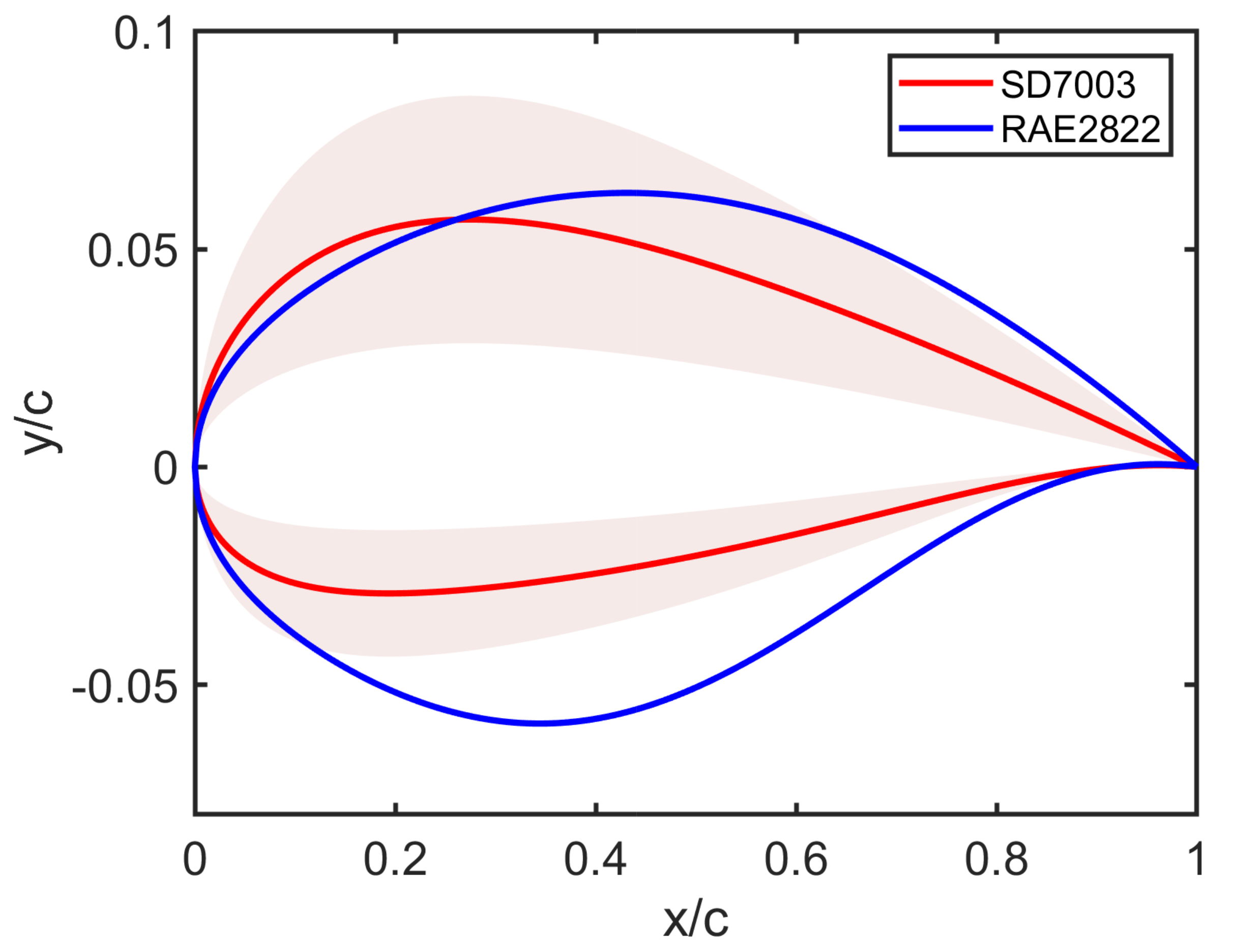
For example, suppose the design baseline is an SD7003 airfoil and a 50% perturbation is performed on the baseline values, and the design target is a supercritical airfoil, such as RAE2822, which requires a flat upper surface and a bent lower surface to compensate for the lift loss caused by the nose’s low curvature. Figure 2 shows that the majority of RAE2822 lies outside of the design space, in the blush region.
Therefore, the issue raised above makes us aware that the target could be missed if the design variables are confined inside inappropriate ranges. One would believe that if the bound values were large enough, the issue could be resolved. Although expanding the bound values or adding more design variables would undoubtedly provide a closer approximation to the theoretical ideal values, the cost of searching, which is calculated as the time required to traverse the whole design space, would increase exponentially. Doronina et al. [38] treated the airfoil parameterization as a data-driven problem, and they separated the variables which control the deformation of airfoil. There are two distinct types of airfoil deformation: (1) The affine deformation, which has four structurally significant deformations to the shape of the airfoil, including changes in thickness, camber, chord length, and twist; (2) high-order deformation, which is a common operation provided by the CST and Hicks–Henne methods and includes undulations on the precise positions. As a linear transformation, the affine deformation can be written as:
s ˜ = M T s ( x ) + b
where M G L 2 , and b R 2 . M stands for an element from the set of all invertible 2 × 2 matrices. Commonly, the airfoil shapes are represented with a discrete form, which can be regarded as a matrix A R n × 2 . That is, a real airfoil shape can be transformed with A M + 1 n , 2 d i a g ( b ) , where 1 n , 2 stands for a n × 2 matrix filled with one. The matrix M ( η ) for η ( 0 , 1 ) can be represented as
( 1 ) M ( η ) 1 0 0 η , ( 2 ) M ( η ) ( 1 η ) 0 0 η , ( 3 ) M ( η ) η 0 0 1 , ( 4 ) M ( η ) c o s ( η π 2 ) s i n ( η π 2 ) s i n ( η π 2 ) c o s ( η π 2 ) ,
respectively.
Obviously, the affine deformation can influence the aerodynamic performance of an airfoil. Due to structural constraints, however, these changes are typically not taken into account. The perturbation on the airfoil induced by the mathematical function, such as the CST and Hicks–Henne methods, has become an very popular means of improving the airfoil aerodynamic capability under some strong constraints, such as twist angle. These adjustments frequently result in sags and crests on the airfoil, which can cause performance variations. The Grassmannian space, denoted as G ( n , q ) , is the subspace of all q-dimensional subspaces of R n , and it is invariant under G L q transformations. In other words, if A ˜ R * n × q stand for a full-rank representative element of the equivalence class [ A ˜ ] G ( n , q ) of all matrices with equivalent column span, the ever element of Grassmannian is a full-rank matrix modulo G L q deformations. Therefore, the affine deformations cannot affect the deformation over G ( n , q ) .
As is well-known, the Grassmannian can be viewed as a quotient topology of orthogonal subgroups, meaning that every element in Grassmannian space has sample covariance proportional to identity matrix [39]. Subsequently, the way given by Doronina et al. [38] to map the physical airfoil shapes, A, to the element in Grassmannian space, A ˜ , is landmark-affine standardization (LAS) [40]. The LAS method normalizes the airfoil shapes (profiles) in order to obtain a zero mean and a sample covariance proportional to identical matrix. For example, an airfoil shape A R * n × 2 has n landmarks, and a thin singular SVD is carried on the shape vector as
( A B ( A ) ) = U Σ V ,
where B ( A ) = 1 n , 2 d i a g ( ( 1 / n ) A 1 n , 1 ) is the discrete center of mass, which is corresponding to every row of A. Let M ˜ = Σ U denote a 2 × 2 invertible matrix. The mapping between physical shape A and its corresponding part A ˜ ( = V ) over the Grassmannian is the affine transformation, that is,
A B ( A ) = A ˜ M ˜ .
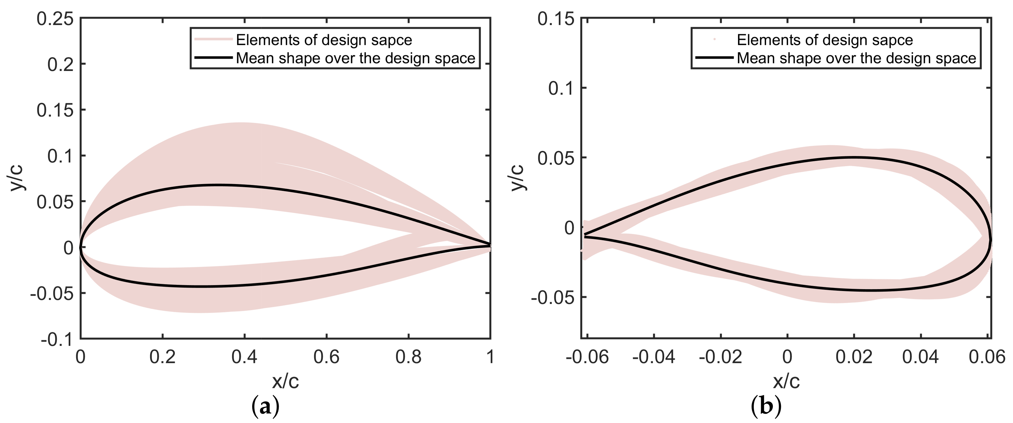
It is very easy to find that A ˜ A ˜ = I 2 , which has been described as a basic feature of Grassmannian space, and we have [ A ˜ ] G ( n , 2 ) . Additionally, the physical shape can be recovered with a linear operation via Equation (10). The advantage of the airfoil design space being sampled into the Grassmannian space is demonstrated by Figure 3.
The shadow in Figure 3 consists of the lower and upper bounds of 7007 airfoils, and this airfoil cluster comes from a thousand samples with a ± 20 % perturbation over the seven baseline airfoils. As shown in Figure 3a, physical airfoils, which are generally specified in Euclidean space, have some discontinuous sections, particularly around the trailing point. This corresponds to the disjoint regions shown in Figure 1. Moreover, the mean shape from the airfoil cluster also departs from the center line of the shadow region. After being aggregated with the LAS method, the scale and translation invariance are brought into the space. It is abundantly clear that the airfoil cluster over the Grassmannian space has normal coordinates, i.e., the maximum and minimum values are similar in different directions. Another advantage is that the varying space has been compacted around the mean shape. A very important step for the LAS method is the Procrustes Analysis, with which can optimally superimpose a set of objects, instead of superimposing them to an arbitrarily selected shape.
The next problem is the principal component analysis (PCA) over the design space to separate out the main elements which can have a large effect on the deformation of airfoils. Because Grassmannian is a curved space, which belongs to Riemannian space, the PCA cannot be directly used on the new dataset. Fletcher et al. [41] presented an idea to apply PCA on manifolds, such as the Grassmannian manifold. The first step is to obtain the intrinsic mean, which is defined as:
μ = arg min A ˜ G ( n , 2 ) i = 1 n d ( A ˜ , A ˜ i ) 2 ,
where G ( n , 2 ) is a Grassmannian manifold, A ˜ stands for an arbitrary element in a collection of points A ˜ 1 , , A ˜ n G ( n , 2 ) and d ( · , · ) denotes the Riemannian distance on G ( n , 2 ) . The way we obtained the intrinsic mean is given by Karcher [42], who treats the computation of the intrinsic mean as solving the minimization problem with the gradient descent algorithm. Defining the cost function as
f ( A ˜ ) = 1 2 n i 1 n d ( A ˜ , A ˜ i ) 2 ,
and the target for us is to find a point a to satisfy f ( A ˜ ) which has a minimum value, i.e., zero. With a size step τ and an previous estimation intrinsic mean μ j , the next estimation is
μ j + 1 = Exp μ j τ N i = 1 n Log μ j ( A ˜ i ) ,
where Exp and Log are the Riemannian exponential map and logarithmic map, respectively. The principal geodesic analysis (PGA) method is to find a sequence of nested geodesic sub-manifolds that have the maximum projected variance of the data, and it is necessary to find the tangent space of G ( n , 2 ) , which is always denoted by T μ G ( n , 2 ) with an intrinsic mean μ . Then, constructing a matrix as
H = 1 n 1 Log μ ( A ˜ 1 ) , , Log μ ( A ˜ N ) ,
and computing the reduced SVD on H up to r d i m ( G ) . The parameter r is the number of design variables corresponds to the first r modes which needs to be held to capture the most variability, e.g., 95%. The new basis for a subspace of the tangent space can be provided by Equation (14). Meanwhile, a neighborhood of zero is defined as U r T μ G ( n , 2 ) , and hence the projection is well-defined for all geodesic submanifolds. As in the expression given by Doronina et al. [38], a compact space U which has the relation U R r can be used to find a normal coordinates t U . Then, a set of all the linear assemblages of the principle components U r t defines a reduced dimensional domain (r-dimension) over the tangent space T μ G ( n , 2 ) with the image of an Riemannian exponential map. Correspondingly, the change over t will give perturbations on the airfoil, which is, obviously, independent of the affine deformations.
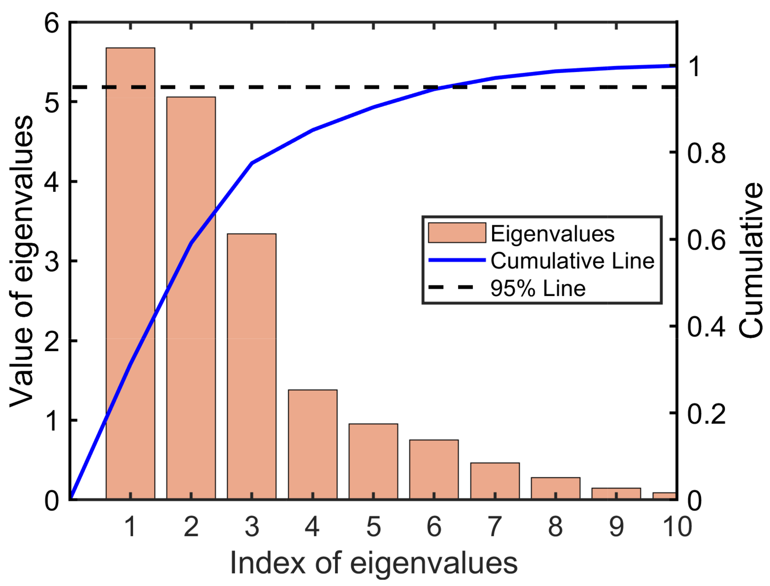
The current dataset that contains 7007 airfoil shapes can be used to give an example. The Karcher mean is plotted in Figure 3b, and it is clear that the value is centered among the elements. Figure 4 is a plot of the first 10 modes of the H over the current dataset, and the first 6 modes capture more than 95% of the total variability, which is a significant reduction from the original 10 dimensions of the design variables. Moreover, over 85 % of the total variability is controlled with the first 4 modes, which must be very beneficial for a quick understanding of the large design space.

3. Airfoil Shape Optimization

In the previous section, the shape parameterization method was described, and in this section, two airfoil optimizations will be performed. Specifically, the optimization frame is comprised of an optimal search module implemented by the stimulated annealing toolbox in MATLAB ® , a computational fluid dynamics (CFD) module implemented by the open source code CFL3D [4], and a mesh deformation module implemented by Pointwise ® . During the search phase, all parameters of the optimization module are frozen. In addition, the turbulence model employed here is Menter’s k ω shear stress transport model [43], and the only variable between cases is the freestream condition. The CST approach utilized in the present work employs 12 parameters to provide a fair description of the airfoil shape, and the upper and lower limits of each design parameter are limited to a 20% increase or decrease in the baseline value. As a data-driven parameterized method, it is impossible to arbitrarily specify the range of design variables. Therefore, the design variables’ limits are derived from the maximum and minimum values of the dataset. As shown in Figure 4, six design variables are utilized to complete the optimization using the Grassmannian shape parameterization (GSP) method.

3.1. Subsonic Airfoil Optimization

Maximizing the lift-to-drag ratio is a common design target for aircraft under subsonic flow conditions, and hence an takeoff freestream velocity, M a = 0.15 , is used in this case. The Reynolds number based on the chord length is 6 million. The bound of farfield is located at 100c and 72,000 grid points is used to discretize the entire computational domain. The distance of the first grid point away from the airfoil is 1 × 10 6 c to guarantee a normalized wall distance y + < 1 .
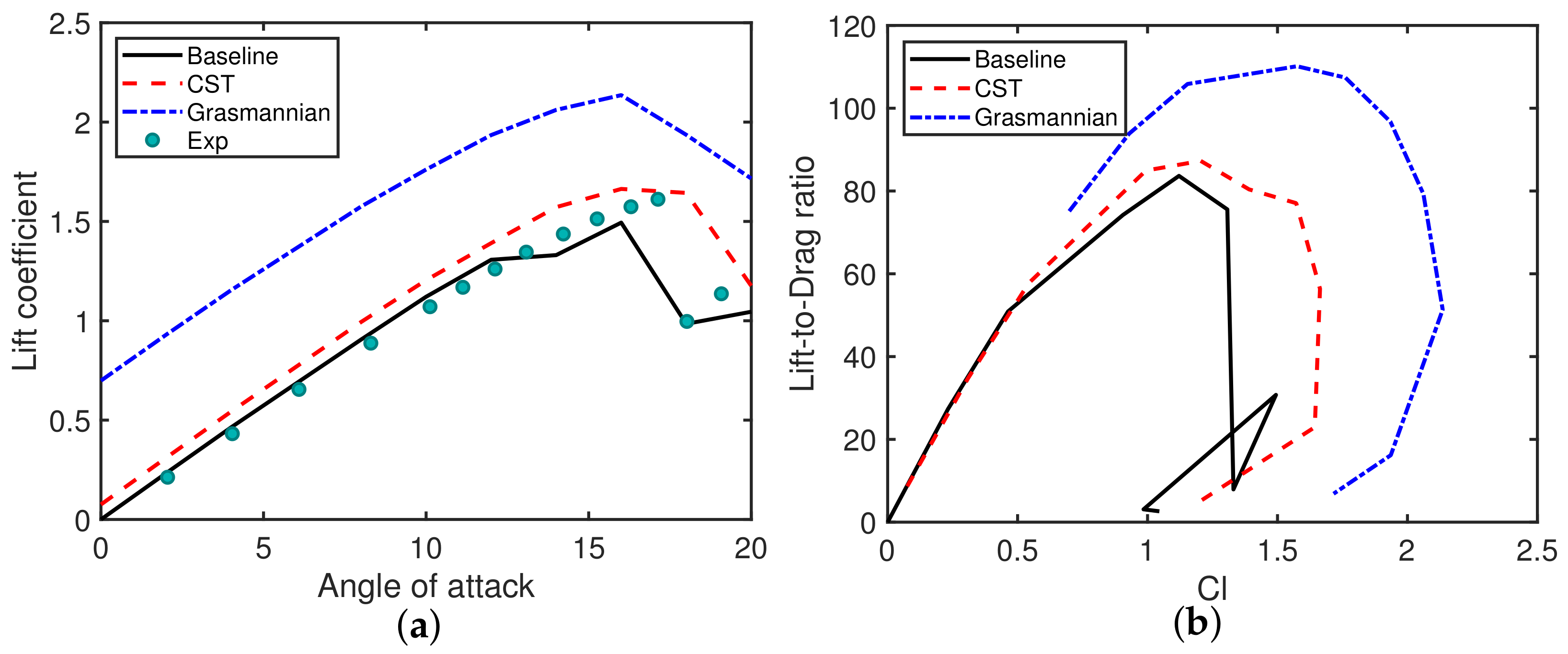
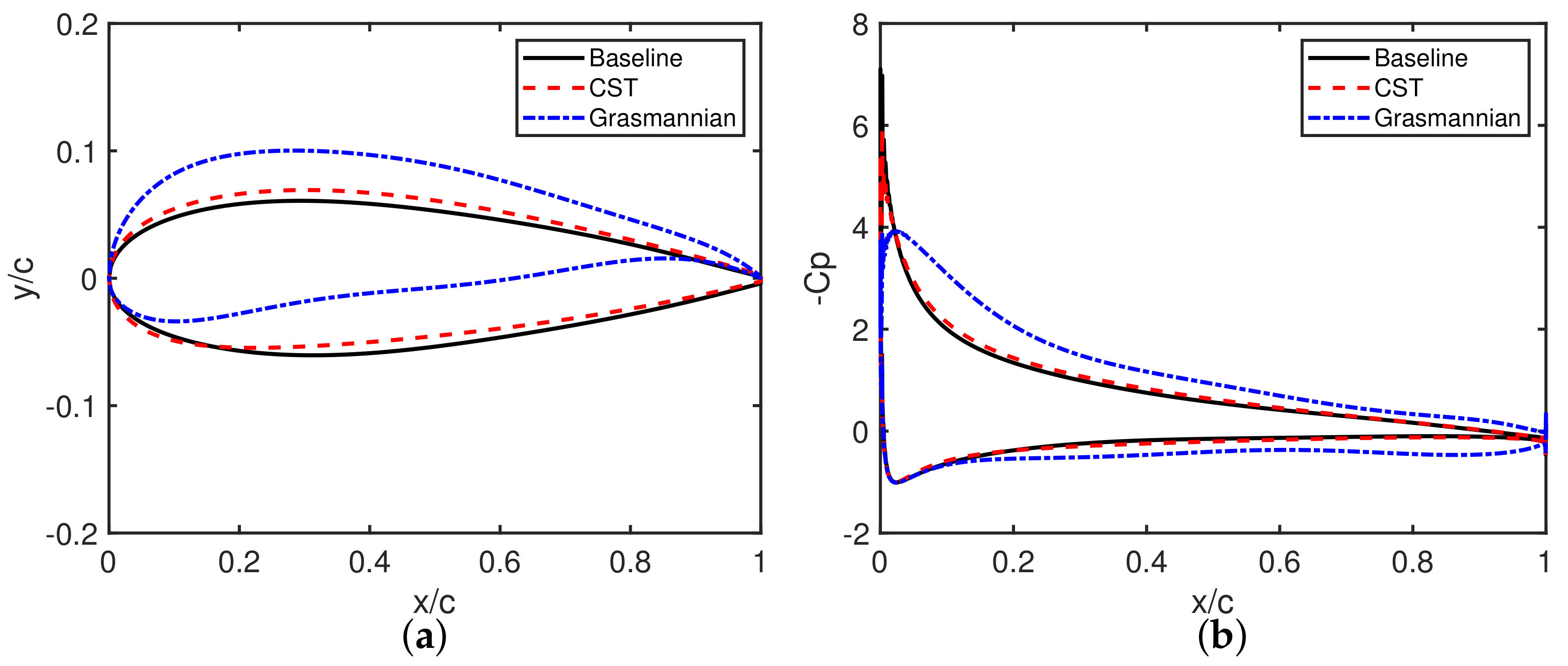
The aerodynamic performance of the airfoils given by optimization was shown in Figure 5a,b. Obviously, the whole lift line is lifted up a lot by the airfoil given by the GSP method, but a little bit by the airfoil given by the CST method. As expressed in the previous section, the GSP method separates the affine deformation from the shape deformation if the matrix M ˜ has no change, which means the scale and translation invariance during the shape deformation. From the view of low-speed airfoil design, a consensus is that the curvature of the upper surface affects the lift-to-drag ratio pretty much if the thickness cannot be changed due to the structural constant. In Figure 6a, the optimized airfoil given by GSP has a larger curvature on the upper surface line and camber on the tail of the lower surface line, and both of these two characters are beneficial to aerodynamic performance. The CST method provides an airfoil with a 1% camber increase for obtaining improved lift force. The slopes of the lift line plotted in Figure 5a from different airfoils are close to each other, which means a similar camber of airfoils. The experimental data come from Ladson [44]. The lift-to-drag ratio, K, demonstrated in Figure 5b, the maximum K is improved from 83 to 110 with the GSP method, and 87 with CST method, respectively. The distribution of pressure coefficient C p of the airfoil at α = 10 deg is demonstrated in Figure 6b, the suction peak is increased and the total area of C p is enlarged from the airfoil given by the GSP method.
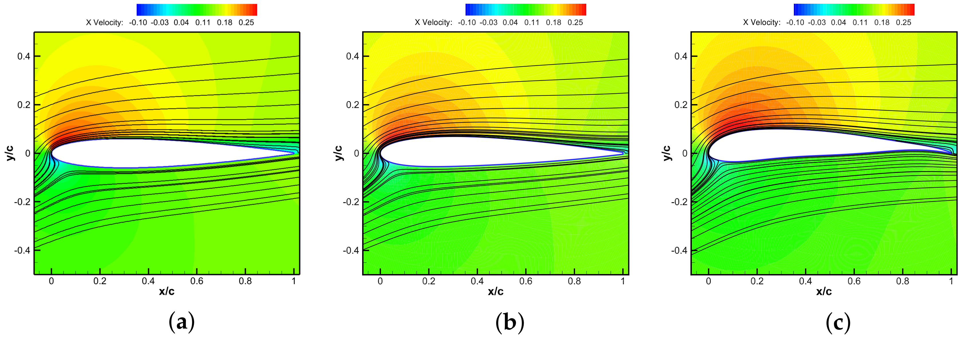
The streamline at a large angle of attack, α = 16 deg , is shown in Figure 7. The velocity contour is very high on the nose of the optimized airfoil from the GSP method. The positive velocity region is enlarged from the baseline to the optimized airfoils.

3.2. Transonic Airfoil Optimization

The most typical transonic airfoil which is used to validate the CFD code is RAE2822. An experiment is performed at M a = 0.729 with α = 2.31 deg [45]. The Reynolds number based on the chord length is 6.5 million.
The minimized drag coefficient C d with a constant lift coefficient C l is very common in the transonic airfoil design process. The supercritical airfoil proposed by Whitcomb et al. [46] was proved to be very good at such flow conditions. The shock wave often appears at the latter part due to the little curvature of the front part of the upper surface. The main principle of optimizing transonic airfoil is smoothing the adverse pressure gradient of the upper surface and increasing the camber of tail to recover the lift.
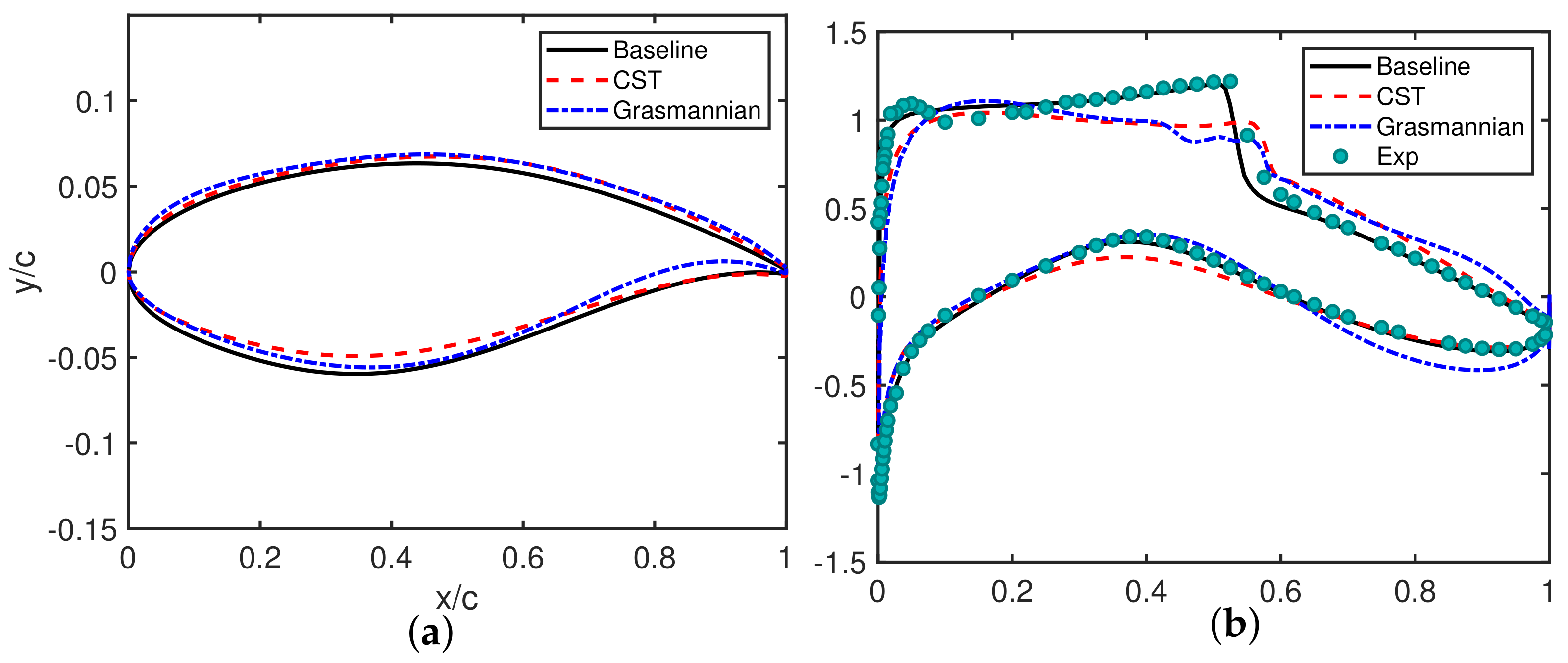
In Figure 8a, a small deformation in the airfoil shape can induce the pressure distribution plotted in Figure 8b, which has very large change, especially at the location with shock wave. The pressure distribution comes from simulations with lift coefficient C l = 0.7429 , and the drag coefficients C d for baseline, CST and GSP models are 0.0123, 0.0101 and 0.099, respectively. Judging from the results, the new method brings very little improvement, however, it must be mentioned here that the shock wave is very sensitive to small-shape deformation. That is, a very little perturbation in the design variables could be enough and the drawback demonstrated in Figure 2 could be covered up. Hence, a general design must be affected by the bound of the design variables.
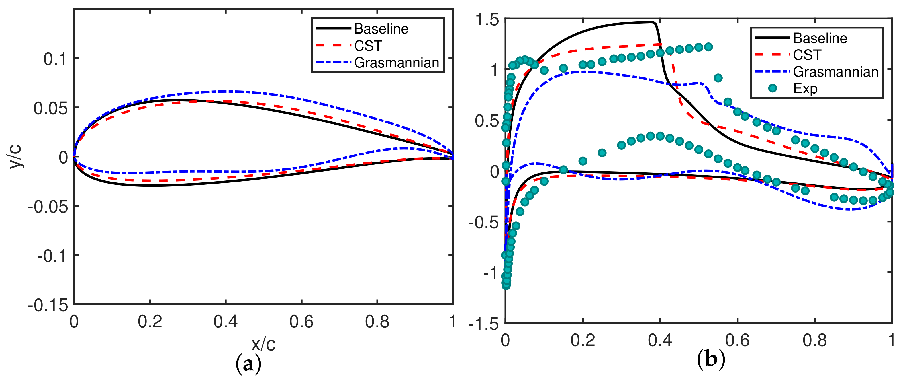
In the new case, the same flow condition is maintained. SD7003, a low-Reynolds number airfoil, which serves as the baseline. Figure 9a depicts the optimized airfoils, and the CST method produces little change on the baseline airfoil. The GSP method, on the other hand, produces an airfoil shape with the characteristics of supercritical airfoils. Meanwhile, the suction peak of a low Reynolds number airfoil is significantly higher than that of a supercritical airfoil, as shown in Figure 9b. Furthermore, the C p distribution produced by the GSP method has a very similar pattern to that shown in Figure 8b, demonstrating that it has a very stable performance even when the baseline airfoil is changed.
The gradient of density is used to demonstrate the strength of the shock wave on the airfoil. The shock wave in Figure 10 shows that the high suction peak induces strong adverse-pressure gradient, which corresponds to a strong shock wave. As the optimized module flattens upper surface, the peak drops and pressure gradient is released.

4. Conclusions

In this study, a method for shape parameterization was utilized to provide a precise and generalized description of airfoil. As a data-driven approach, a wide variety of airfoil types can be included prior to optimization, and this advantage can give the designer a sense of what the types of the optimized airfoil will be. However, the disjointed design space, which is caused by the non-normalized perturbation of design variables, could hinder the optimized method from achieving the best value. The benefit of transforming an airfoil from Euclidean space to Grassmannian space is that, as a result of the landmark-affine deformation, the design space can be closely matched. The dimensionality of the design space can also be reduced to a single digit using the PGA method. The Karcher-centered domain of normal coordinates provides an advantage in that the new method has the shortest routine to any element in the space, which, presumably, requires the least amount of time to locate the optimal shape in the design space. In the meantime, the affine deformation, which cannot be prevented with traditional methods such as CST, can be separated with the new method, and the design must be enhanced by the regularization against non-physical deformations.
We demonstrated that the new method is very robust at both the subsonic and transonic levels through the use of numerical processes of a variety of cases that were optimized. The disadvantage of the traditional parameterization method, which is that it heavily relies on the bounds of design variables, can now be overcome.

Author Contributions

Data curation, B.P.; Methodology, X.L.; Software, G.C.; Writing—original draft, Y.Z. All authors have read and agreed to the published version of the manuscript.

Funding

This research was funded by Young Scientists Fund of the National Natural Science Foundation of China (Grant No. 11602199).

Data Availability Statement

Not applicable.

Conflicts of Interest

The authors declare no conflict of interest.

Abbreviations

The following abbreviations are used in this manuscript:
PARSECParametric section
CSTClass-shape function transformation
DRDimension reduction
PODProper orthogonal decomposition
SVDSingular value decomposition
ASMActive subspace method
QOIQuality of interest
LASLandmark-affine standardization
PCAPrincipal component analysis
PGAPrincipal geodesic analysis
GSPGrassmannian shape parameterization

References

  1. Lighthill, M. A New Method of Two-Dimensional Aerodynamics Design. Aeronautical Research Council. 1945. Available online: https://reports.aerade.cranfield.ac.uk/handle/1826.2/3876 (accessed on 21 October 2014).
  2. Volpe, G.; Melnik, R. Role of constraints in inverse design for transonic airfoils. AIAA J. 1984, 22, 1770–1778. [Google Scholar] [CrossRef]
  3. Drela, M.; Giles, M.B. Viscous-inviscid analysis of transonic and low Reynolds number airfoils. AIAA J. 1987, 25, 1347–1355. [Google Scholar] [CrossRef]
  4. Krist, S.L. CFL3D User’s Manual, Version 5.0; National Aeronautics and Space Administration, Langley Research Center: Hampton, VA, USA, 1998. [Google Scholar]
  5. Jameson, A.; Reuther, J. Control theory based airfoil design using the Euler equations. In Proceedings of the 5th Symposium on Multidisciplinary Analysis and Optimization, Panama City, FL, USA, 7–9 September 1994; p. 4272. [Google Scholar]
  6. Jameson, A.; Kim, S. Reduction of the adjoint gradient formula for aerodynamic shape optimization problems. AIAA J. 2003, 41, 2114–2129. [Google Scholar] [CrossRef]
  7. Zingg, D.W.; Nemec, M.; Pulliam, T.H. A comparative evaluation of genetic and gradient-based algorithms applied to aerodynamic optimization. Eur. J. Comput. Mech./Revue Européenne de Mécanique Numérique 2008, 17, 103–126. [Google Scholar] [CrossRef] [Green Version]
  8. Nemec, M.; Zingg, D.W.; Pulliam, T.H. Multipoint and multi-objective aerodynamic shape optimization. AIAA J. 2004, 42, 1057–1065. [Google Scholar] [CrossRef]
  9. He, X.; Li, J.; Mader, C.A.; Yildirim, A.; Martins, J.R. Robust aerodynamic shape optimization—From a circle to an airfoil. Aerosp. Sci. Technol. 2019, 87, 48–61. [Google Scholar] [CrossRef]
  10. Zhang, Z.; De Gaspari, A.; Ricci, S.; Song, C.; Yang, C. Gradient-Based Aerodynamic Optimization of an Airfoil with Morphing Leading and Trailing Edges. Appl. Sci. 2021, 11, 1929. [Google Scholar] [CrossRef]
  11. Venter, G.; Sobieszczanski-Sobieski, J. Particle swarm optimization. AIAA J. 2003, 41, 1583–1589. [Google Scholar] [CrossRef] [Green Version]
  12. Pehlivanoglu, Y.V.; Yagiz, B.; Kandil, O.; Baysal, O. Particle swarm optimization of suction and blowing on airfoils at transonic speeds. J. Aircr. 2010, 47, 1955–1965. [Google Scholar] [CrossRef]
  13. Wang, Y.y.; Zhang, B.q.; Chen, Y.c. Robust airfoil optimization based on improved particle swarm optimization method. Appl. Math. Mech. 2011, 32, 1245–1254. [Google Scholar] [CrossRef]
  14. Li, J.; Gao, Z.; Huang, J.; Zhao, K. Robust design of NLF airfoils. Chin. J. Aeronaut. 2013, 26, 309–318. [Google Scholar] [CrossRef] [Green Version]
  15. Yang, B.; Xu, Q.; He, L.; Zhao, L.; Gu, C.G.; Ren, P. A novel global optimization algorithm and its application to airfoil optimization. J. Turbomach. 2015, 137, 041011. [Google Scholar] [CrossRef]
  16. Bashir, M.; Longtin-Martel, S.; Botez, R.M.; Wong, T. Aerodynamic Design Optimization of a Morphing Leading Edge and Trailing Edge Airfoil–Application on the UAS-S45. Appl. Sci. 2021, 11, 1664. [Google Scholar] [CrossRef]
  17. Sobieczky, H. Parametric airfoils and wings. In Recent Development of Aerodynamic Design Methodologies; Springer: Berlin/Heidelberg, Germany, 1999; pp. 71–87. [Google Scholar]
  18. Masters, D.A.; Taylor, N.J.; Rendall, T.; Allen, C.B.; Poole, D.J. Geometric comparison of aerofoil shape parameterization methods. AIAA J. 2017, 55, 1575–1589. [Google Scholar] [CrossRef] [Green Version]
  19. Hicks, R.M.; Henne, P.A. Wing design by numerical optimization. J. Aircr. 1978, 15, 407–412. [Google Scholar] [CrossRef]
  20. Ahn, J.; Kim, H.J.; Lee, D.H.; Rho, O.H. Response surface method for airfoil design in transonic flow. J. Aircr. 2001, 38, 231–238. [Google Scholar] [CrossRef]
  21. Zhou, C.; Wang, Z.; Zhi, J.; Kretov, A. Aerothermodynamic Optimization of Aerospace Plane Airfoil Leading Edge. J. Aerosp. Technol. Manag. 2017, 9, 503–509. [Google Scholar] [CrossRef]
  22. Xu, S.; Chen, H.; Zhang, J. A study of Nash-EGO algorithm for aerodynamic shape design optimizations. Struct. Multidiscip. Optim. 2019, 59, 1241–1254. [Google Scholar] [CrossRef]
  23. Yirtici, O.; Tuncer, I.H. Aerodynamic shape optimization of wind turbine blades for minimizing power production losses due to icing. Cold Reg. Sci. Technol. 2021, 185, 103250. [Google Scholar] [CrossRef]
  24. Zhou, S.; Zhou, H.; Yang, K.; Dong, H.; Gao, Z. Research on blade design method of multi-blade centrifugal fan for building efficient ventilation based on Hicks-Henne function. Sustain. Energy Technol. Assessments 2021, 43, 100971. [Google Scholar] [CrossRef]
  25. Kulfan, B.M. Universal parametric geometry representation method. J. Aircr. 2008, 45, 142–158. [Google Scholar] [CrossRef]
  26. Zhu, F.; Qin, N. Intuitive class/shape function parameterization for airfoils. AIAA J. 2014, 52, 17–25. [Google Scholar] [CrossRef]
  27. Liu, Z.; Dong, L.; Moschetta, J.M.; Zhao, J.; Yan, G. Optimization of nano-rotor blade airfoil using controlled elitist NSGA-II. Int. J. Micro Air Veh. 2014, 6, 29–42. [Google Scholar] [CrossRef] [Green Version]
  28. Liu, X.; He, W. Airfoil optimization design based on the pivot element weighting iterative method. Algorithms 2018, 11, 163. [Google Scholar] [CrossRef] [Green Version]
  29. Akram, M.T.; Kim, M.H. Aerodynamic shape optimization of NREL S809 airfoil for wind turbine blades using reynolds-averaged navier stokes model—Part II. Appl. Sci. 2021, 11, 2211. [Google Scholar] [CrossRef]
  30. Cinquegrana, D.; Iuliano, E. Investigation of adaptive design variables bounds in dimensionality reduction for aerodynamic shape optimization. Comput. Fluids 2018, 174, 89–109. [Google Scholar] [CrossRef]
  31. Sripawadkul, V.; Padulo, M.; Guenov, M. A comparison of airfoil shape parameterization techniques for early design optimization. In Proceedings of the 13th AIAA/ISSMO Multidisciplinary Analysis Optimization Conference, Fort Worth, TX, USA, 13–15 September 2010; p. 9050. [Google Scholar]
  32. Poole, D.J.; Allen, C.B.; Rendall, T. Aerofoil design variable extraction for aerodynamic optimization. In Proceedings of the 21st AIAA Computational Fluid Dynamics Conference, San Diego, CA, USA, 24–27 June 2013; p. 2705. [Google Scholar]
  33. Poole, D.J.; Allen, C.B.; Rendall, T.C. Metric-based mathematical derivation of efficient airfoil design variables. AIAA J. 2015, 53, 1349–1361. [Google Scholar] [CrossRef]
  34. Grey, Z.J.; Constantine, P.G. Active subspaces of airfoil shape parameterizations. AIAA J. 2018, 56, 2003–2017. [Google Scholar] [CrossRef]
  35. Li, J.; Cai, J.; Qu, K. Surrogate-based aerodynamic shape optimization with the active subspace method. Struct. Multidiscip. Optim. 2019, 59, 403–419. [Google Scholar] [CrossRef]
  36. Li, J.; Zhang, M. Adjoint-free aerodynamic shape optimization of the common research model wing. AIAA J. 2021, 59, 1990–2000. [Google Scholar]
  37. Li, J.; Zhang, M.; Tay, C.M.J.; Liu, N.; Cui, Y.; Chew, S.C.; Khoo, B.C. Low-Reynolds-number airfoil design optimization using deep-learning-based tailored airfoil modes. Aerosp. Sci. Technol. 2022, 121, 107309. [Google Scholar] [CrossRef]
  38. Doronina, O.A.; Grey, Z.J.; Glaws, A. Grassmannian Shape Representations for Aerodynamic Applications. arXiv 2022, arXiv:2201.04649. [Google Scholar]
  39. Edelman, A.; Arias, T.A.; Smith, S.T. The geometry of algorithms with orthogonality constraints. SIAM J. Matrix Anal. Appl. 1998, 20, 303–353. [Google Scholar] [CrossRef]
  40. Bryner, D.; Klassen, E.; Le, H.; Srivastava, A. 2D affine and projective shape analysis. IEEE Trans. Pattern Anal. Mach. Intell. 2013, 36, 998–1011. [Google Scholar] [CrossRef]
  41. Fletcher, P.T.; Lu, C.; Pizer, S.M.; Joshi, S. Principal geodesic analysis for the study of nonlinear statistics of shape. IEEE Trans. Med. Imaging 2004, 23, 995–1005. [Google Scholar] [CrossRef]
  42. Karcher, H. Riemannian center of mass and so called karcher mean. arXiv 2014, arXiv:1407.2087. [Google Scholar]
  43. Menter, F.R. Improved Two-Equation k-Omega Turbulence Models for Aerodynamic Flows; Technical Report; NASA Ames Research Center Moffett Field: Santa Clara, CA, USA, 1992. [Google Scholar]
  44. Ladson, C.L. Effects of Independent Variation of Mach and Reynolds Numbers on the Low-Speed Aerodynamic Characteristics of the NACA 0012 Airfoil Section; National Aeronautics and Space Administration, Scientific and Technical Information (STI) Program: Hampton, VA, USA, 1988; Volume 4074. [Google Scholar]
  45. Cook, P.; McDonald, M.; Firmin, M. Aerofoil Rae 2822-Pressure Distributions, and Boundary Layer and Wake Measurements. Experimental Data Base For Computer Program Assessment; AGARD Report AR; AGARD: Neuilly-sur-Seine, France, 1979; Volume 138. [Google Scholar]
  46. Whitcomb, R.T. Review of NASA supercritical airfoils. In Proceedings of the International Council of the Aeronautical Sciences Congress, Haifa, Israel, 25–30 August 1974. Number ICAS PAPER 74-10. [Google Scholar]
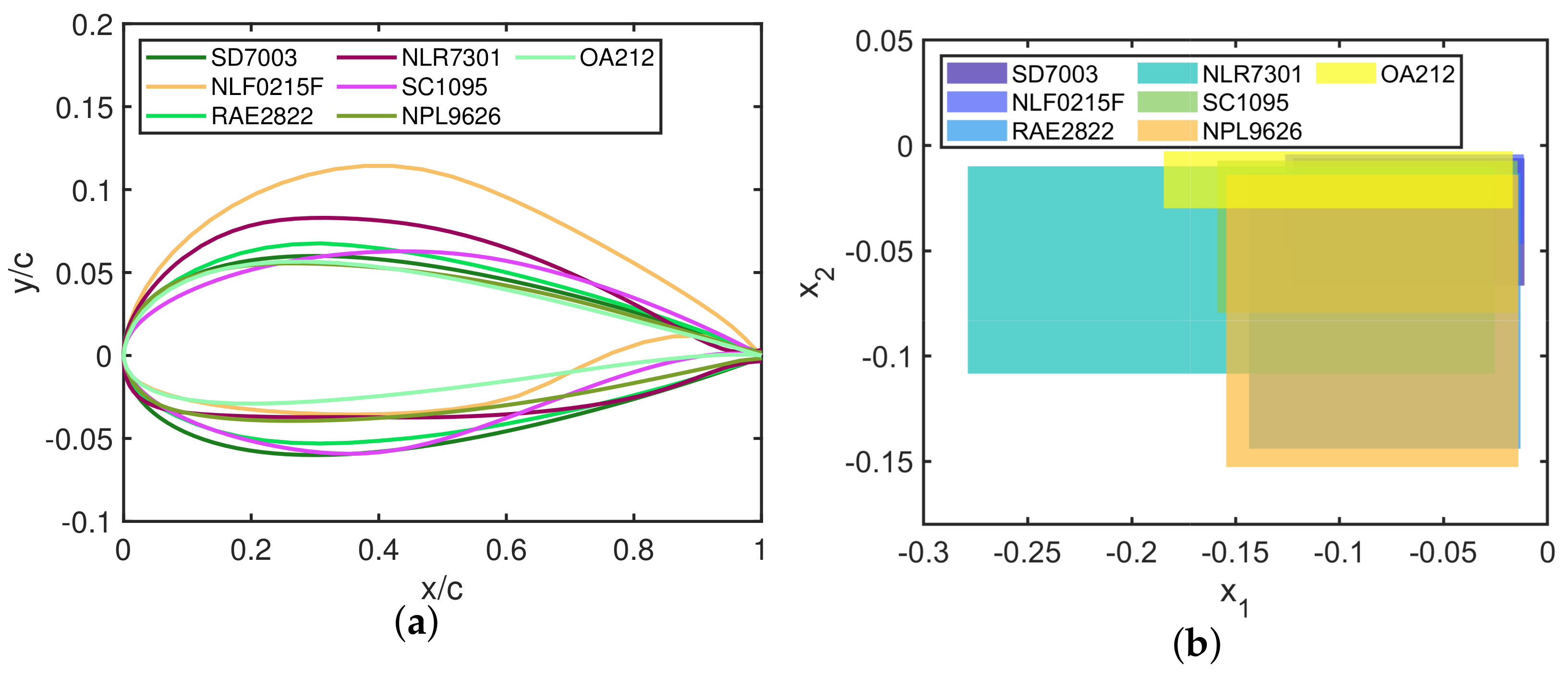
Figure 1. The baseline airfoil classes and part of design space. (a) seven baseline airfoils; (b) the margin of 2 out of 10 CST parameters.
Energies 15 07722 g001
Figure 2. Demonstration of baseline airfoil, design space and target airfoil.
Energies 15 07722 g002
Figure 3. Mean shape and design space: (a) physical space; and (b) Grassmannian space.
Energies 15 07722 g003
Figure 4. Demonstration of the eigenvalues from the modes of variation and their cumulative sums.
Energies 15 07722 g004
Figure 5. Aerodynamic performance of the optimized airfoils under subsonic conditions: (a) C l vs. α ; and (b) C l vs. K.
Energies 15 07722 g005
Figure 6. Comparison of the geometry and pressure coefficient of the subsonic case: (a) airfoil shape; (b) pressure distribution.
Energies 15 07722 g006
Figure 7. The streamline of the airfoils at α = 16 deg . The contour is colored with streamwise velocity: (a) baseline; (b) CST; and (c) Grassmannian.
Energies 15 07722 g007
Figure 8. Comparison of the geometry and pressure coefficient of the transonic case: (a) Airfoil shape; and (b) Pressure distribution.
Energies 15 07722 g008
Figure 9. Comparison of the geometry and pressure coefficient of the transonic case of the optimization from SD7003: (a) airfoil shape; (b) pressure distribution.
Energies 15 07722 g009
Figure 10. The gradient of density along the streamwise direction on the SD7003 airfoil: (a) baseline; (b) CST; and (c) Grassmannian.
Energies 15 07722 g010
Table 1. The components of vector x corresponding to the specific airfoils.
Airfoil x 1 x 2 x 3 x 4 x 5
Lower Surface
SD7003−0.1113−0.0605−0.0611−0.05610.0217
NLF0215F−0.1147−0.0424−0.1336−0.18150.3003
RAE2822−0.1305−0.1309−0.2340−0.06650.0325
NLR7301−0.2535−0.0985−0.3397−0.13880.1041
SC1095−0.1444−0.0722−0.1158−0.0858−0.0929
NPL9626−0.1405−0.1388−0.1419−0.1111−0.1558
OA212−0.1678−0.0271−0.1266−0.1237−0.1613
Airfoil x 6 x 7 x 8 x 9 x 10
Upper Surface
SD70030.15850.16420.12030.12400.1092
NLF0215F0.22780.25810.41420.19650.3958
RAE28220.12770.14040.18770.19680.1990
NLR73010.31200.10510.31630.25420.2345
SC10950.17970.13340.13180.14170.1245
NPL96260.17080.18490.17630.12680.1840
OA2120.18900.28060.11160.35480.0038
Publisher’s Note: MDPI stays neutral with regard to jurisdictional claims in published maps and institutional affiliations.