
Development of a Simple Methodology Using Meteorological Data to Evaluate Concentrating Solar Power Production Capacity


Abstract
1. Introduction
2. Methodology
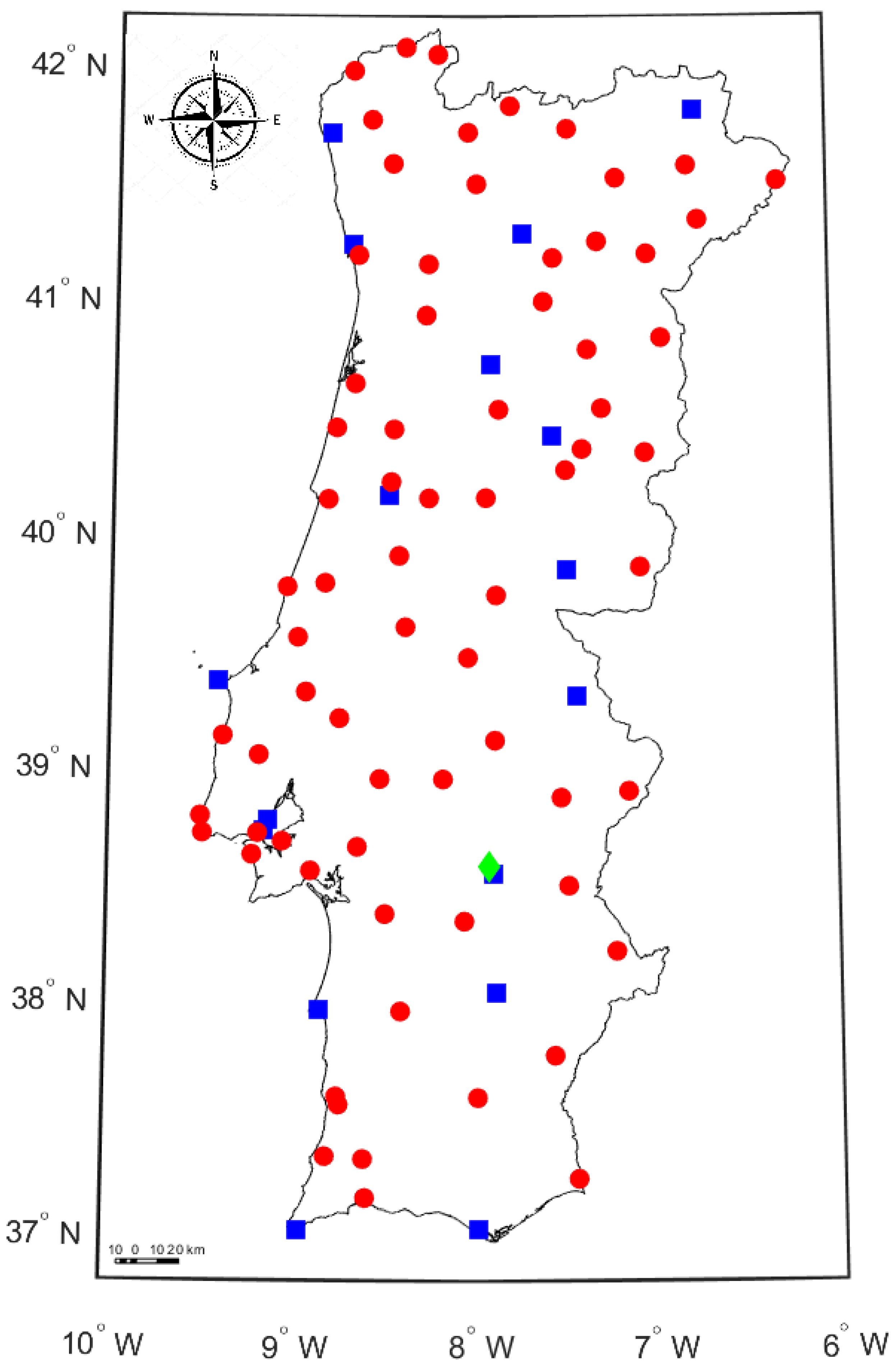
2.1. Measurements
2.2. Data Pre-Processing
- Z < 85°;
- GHI > 0, DHI > 0, DNI ≥ 0;
- DNI < 1100 + 0.03 × Elev;
- DNI < E0n;
- DHI < 0.95 × E0n × cos1.2 Z + 50;
- GHI < 1.50 × E0n × cos1.2 Z + 100;
- DHI/GHI < 1.05 for GHI > 50 and Z < 75°;
- DHI/GHI < 1.10 for GHI > 50 and Z > 75°.
2.3. Engerer Model Application
2.4. Data Post-Processing
2.5. Data Gap Filling
2.6. Typical Meteorological Year Calculation
2.7. The Power Plant Model
3. Results and Discussion
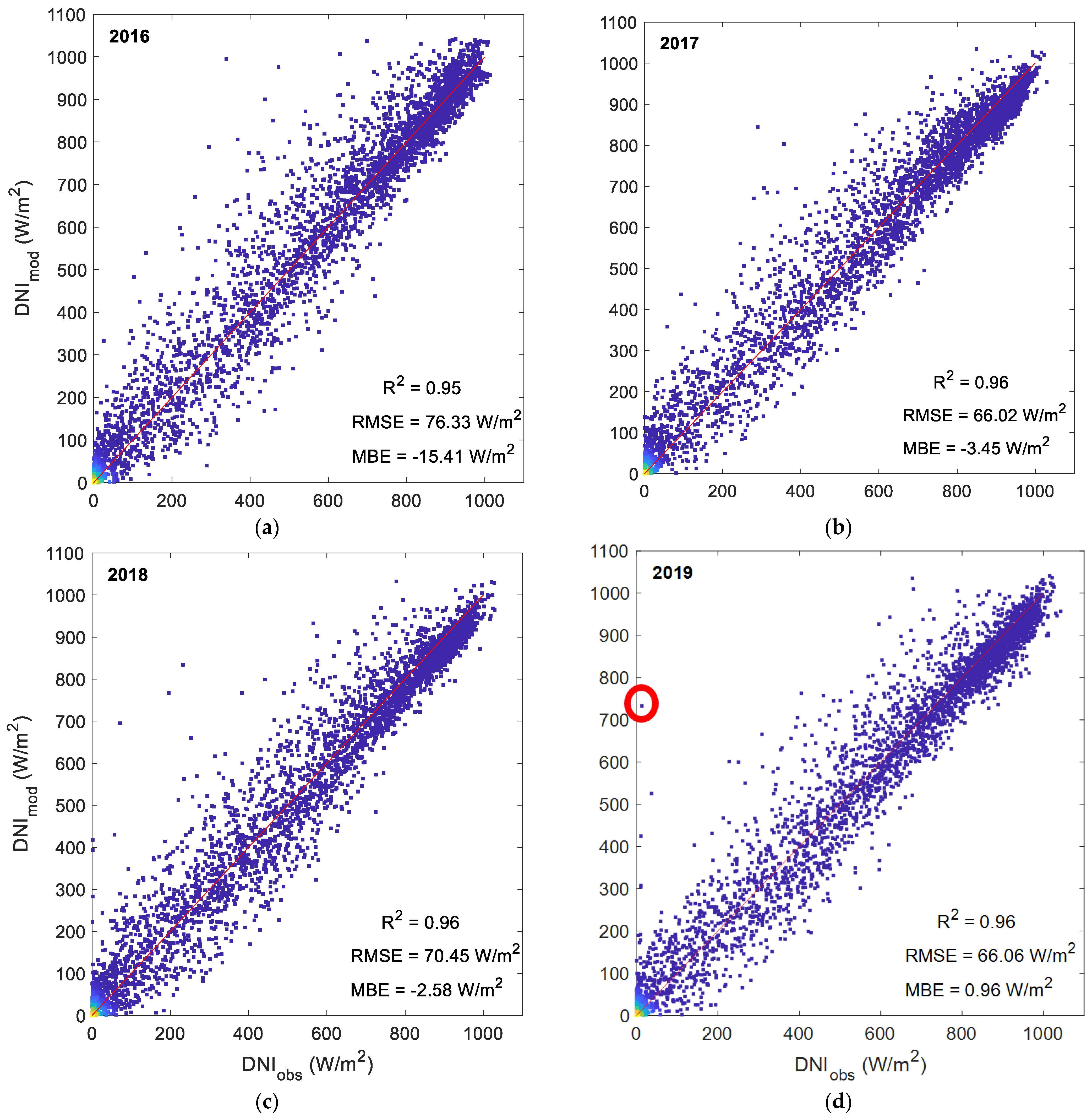
3.1. DNI Validation and Calibration
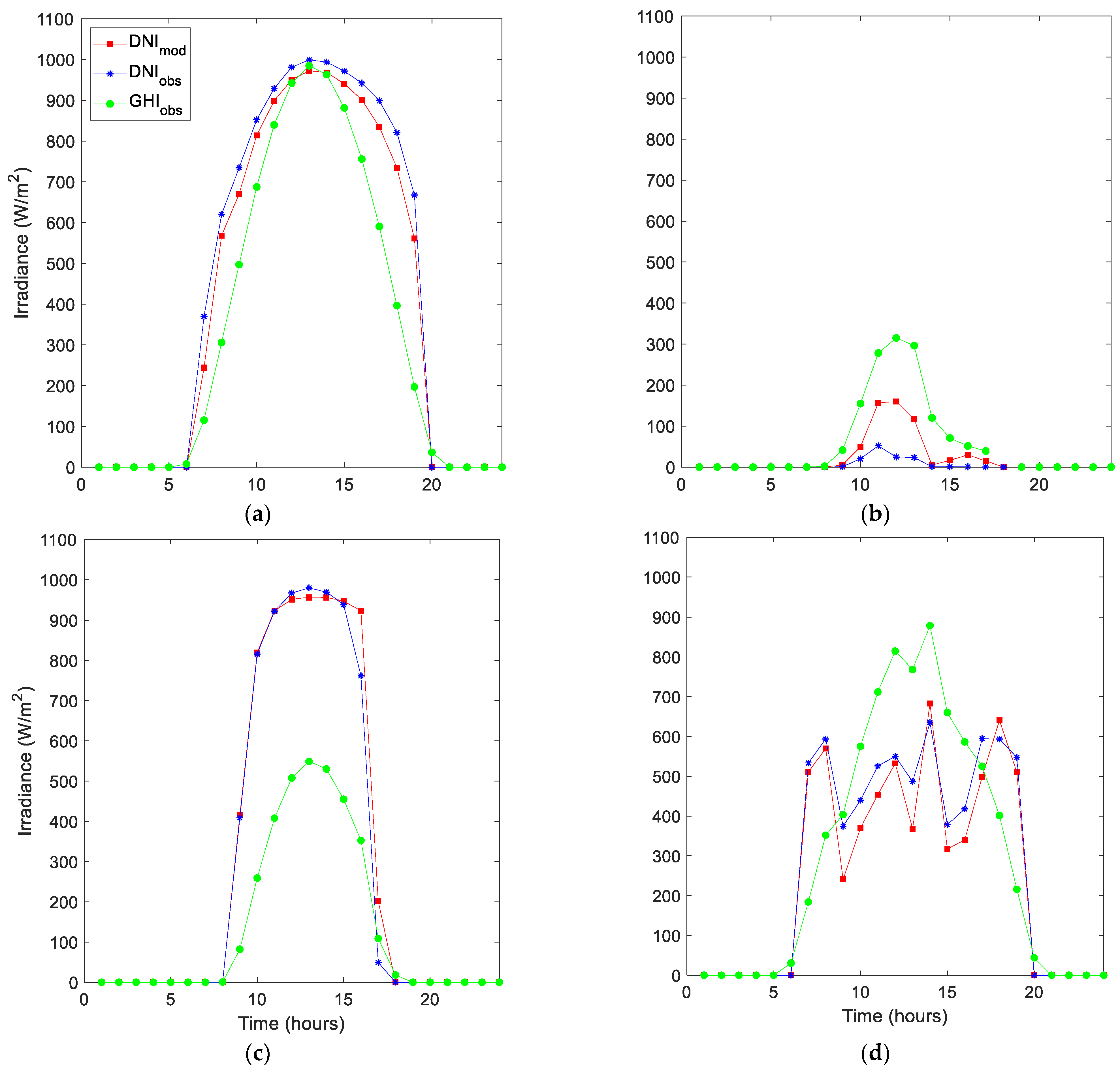
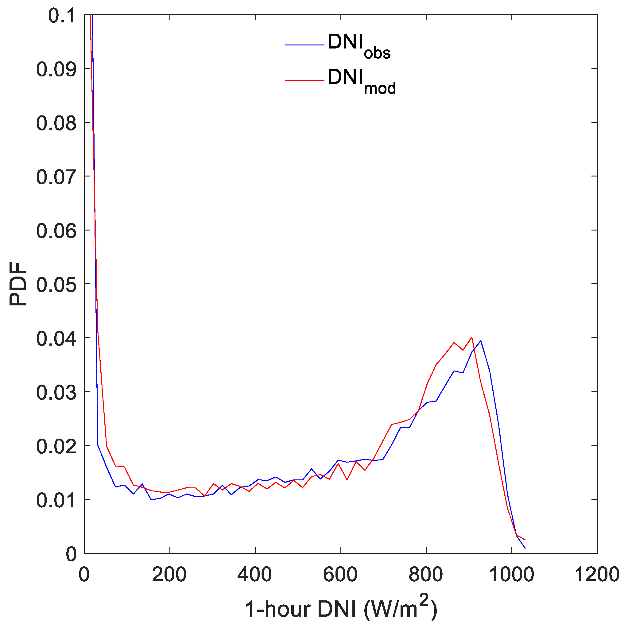
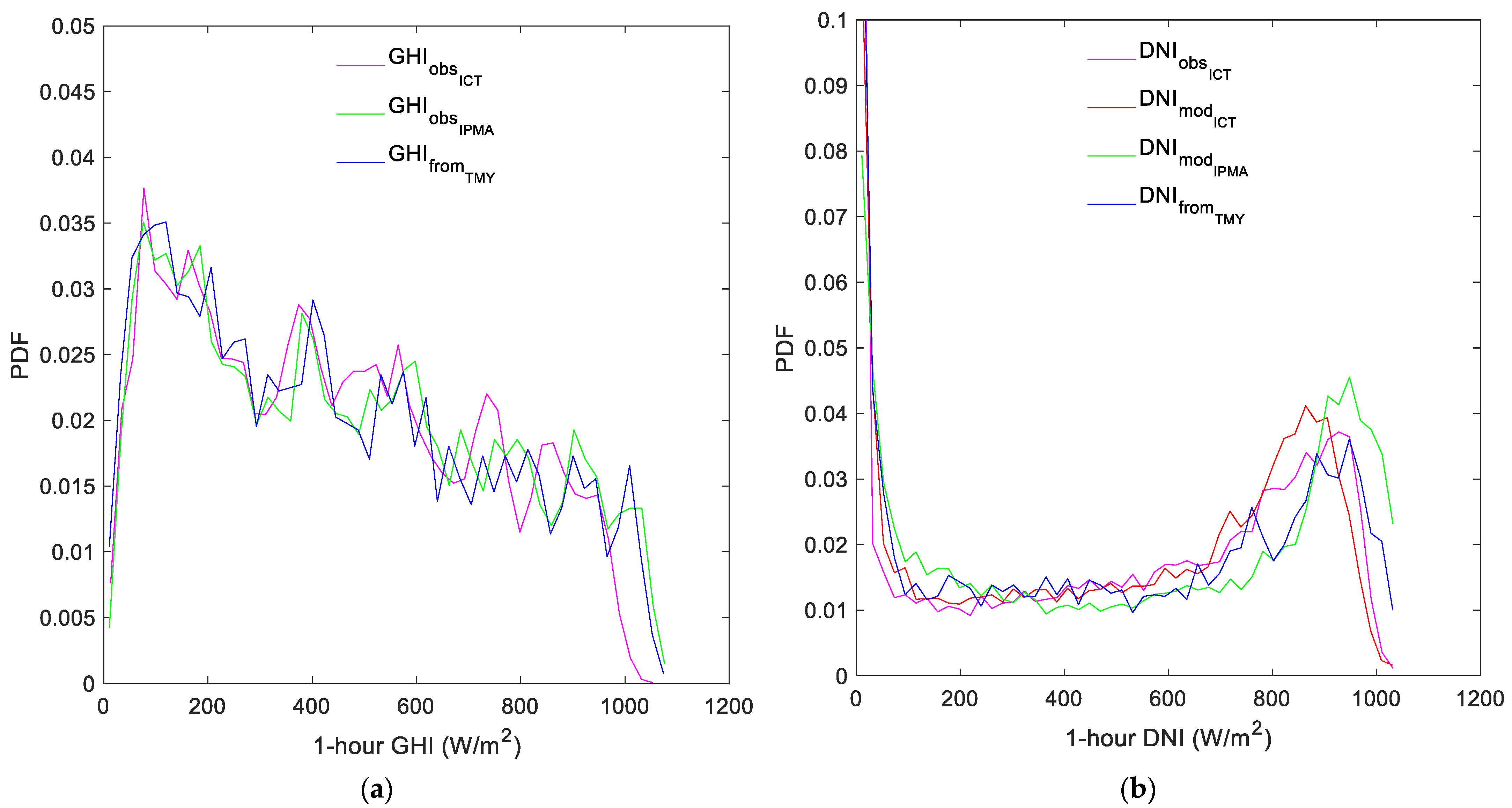
3.2. DNI Estimation
3.3. TMY Calculation
3.4. IPMA’s Main Stations: DNI Availabilities and CF Estimations
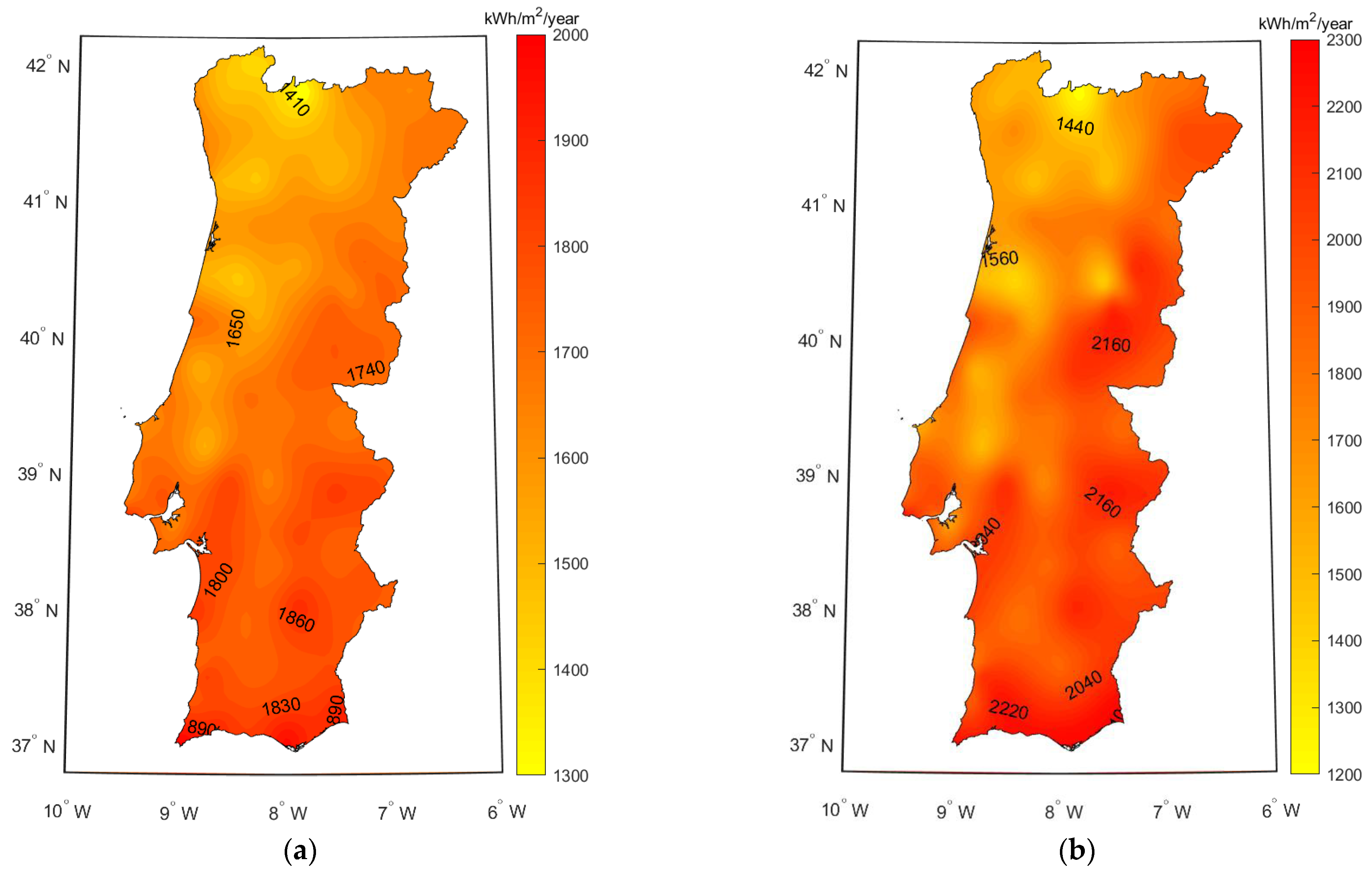
3.5. PMA Network: Assessment of Solar Availability
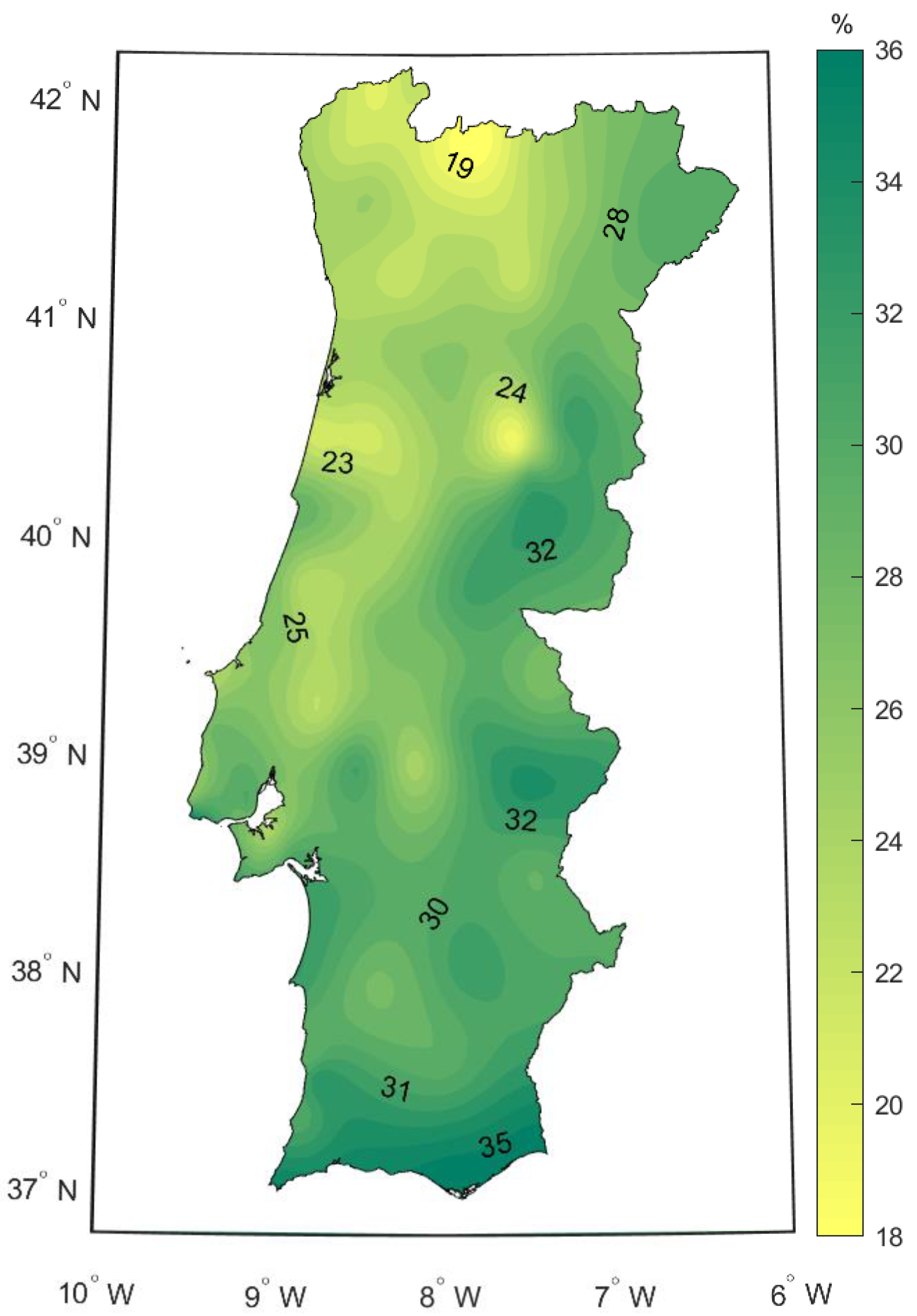
3.6. IPMA Network: Production Capacity of CSP Plants
4. Implications for Decision Making
5. Conclusions
- DNI values modelled from GHI with the use of Engerer2 show very good agreement with the observations;
- GHI and DNI annual availabilities estimated for the IPMA network show very good accordance with previous values found in the literature;
- Annual DNI availabilities and CFs were found to be as high as ~2310 kWh/m2 and ~36.2% in Castro Marim and in Faro cities in Algarve, respectively.
- DNI availability and CF mapping showed the existence of three preferential regions for CSP installation: two in Southern Portugal—Alentejo and Algarve regions; and one in eastern central Portugal—Beira Interior region);
Author Contributions
Funding
Institutional Review Board Statement
Informed Consent Statement
Acknowledgments
Conflicts of Interest
Nomenclature
| Coefficients of Engerer model | |
| Relative difference of DNI availability [%] | |
| Deviation between the observed value of kt at surface and the one obtained under clear sky [dimensionless] | |
| σ | standard deviation |
| AST | Apparent solar time [h] |
| C | Lower asymptote [dimensionless] |
| CF | Capacity factor [%] |
| Diffuse Horizontal Irradiance [W/m2] | |
| Direct Normal Irradiance [W/m2] | |
| Direct Normal Irradiance at clear-sky [W/m2] | |
| Global Horizontal Irradiance [W/m2] | |
| Global Horizontal Irradiance at clear-sky [W/m2] | |
| adjusted modelled DNI [W/m2] | |
| DNI availability [kWh/m2/year] | |
| GHI availability [kWh/m2/year] | |
| Elev | Elevation of each station [m] |
| Irradiance at the top of the atmosphere | |
| diffuse fraction [dimensionless] | |
| portion of attributed in case of cloud enhancement [dimensionless] | |
| Clearness index [dimensionless] | |
| Clearness index at clear-sky [dimensionless] | |
| MAE | Mean Absolute Error [W/m2] |
| MBE | Mean Bias Error [W/m2] |
| Atmospheric pressure [hPa] | |
| Precipitation [mm] | |
| r | correlation coefficient [dimensionless] |
| R2 | coefficient of determination [dimensionless] |
| Relative Humidity [%] | |
| RMSE | Root Mean Square Error [W/m2] |
| Ambient Temperature [°C] | |
| Wind Speed [m/s] | |
| Z | Zenith angle [°] |
| CDF | Cumulative Frequency Distribution Function |
| CSP | Concentrating Solar Power |
| FS | Finkelstein-Schafer statistic |
| IPMA | Instituto Português do Mar e da Atmosfera |
| MRM | Multivariate Regression Model |
| SAM | System Advisor model |
| TMM | Typical Meteorological Month |
| TMY | Typical Meteorological Year |
Appendix A

| Station Names | Latitude (°N) | Longitude (°W) | Elevation (m) | Period of Data (Years) | Eb (kWh/m2/year) | Eg (kWh/m2/year) | CF (%) | Annual Power Generation (GWh/year) |
|---|---|---|---|---|---|---|---|---|
| Cabo Carvoeiro/Farol | 39.36 | −9.41 | 32.00 | 9.01 | 1521.87 | 1625.36 | 22.8 | 99.79 |
| Sagres/Quartel da Marinha | 37.01 | −8.95 | 22.85 | 10.02 | 2245.30 | 1988.94 | 35.2 | 154.35 |
| Lisboa/Geofísico | 38.72 | −9.15 | 77.00 | 13.30 | 1888.81 | 1755.44 | 29.1 | 127.50 |
| Sines/Monte Chãos | 37.95 | −8.84 | 103.00 | 19.72 | 2024.39 | 1854.89 | 31.9 | 139.87 |
| Viana do Castelo/Meadela | 41.71 | −8.80 | 16.00 | 4.79 | - | - | - | - |
| Porto/Pedras Rubras | 41.23 | −8.68 | 69.00 | 17.63 | 1624.47 | 1603.49 | 24.2 | 105.95 |
| Coimbra/Aeródromo | 40.16 | −8.47 | 171.00 | 17.01 | 1809.43 | 1645.21 | 25.7 | 112.64 |
| Faro/Aeroporto | 37.02 | −7.97 | 5.00 | 16.96 | 2280.66 | 1963.54 | 36.2 | 158.71 |
| Évora/Aeródromo | 38.54 | −7.89 | 247.56 | 13.21 | 2030.14 | 1808.25 | 30.3 | 132.53 |
| Viseu/Aeródromo | 40.71 | −7.90 | 644.37 | 13.97 | 1786.90 | 1622.90 | 26.1 | 114.49 |
| Beja | 38.03 | −7.87 | 246.00 | 17.02 | 2145.45 | 1878.65 | 31.8 | 139.48 |
| Vila Real/Aeródromo | 41.27 | −7.72 | 561.00 | 19.92 | 1603.01 | 1561.46 | 23.6 | 103.28 |
| Penhas Douradas/Observatório | 40.41 | −7.56 | 1380.00 | 14.80 | 1467.85 | 1672.30 | 19.4 | 84.98 |
| Castelo Branco | 39.84 | −7.48 | 386.00 | 11.83 | 2078.07 | 1769.59 | 31.2 | 136.84 |
| Portalegre | 39.29 | −7.42 | 597.00 | 17.07 | 1875.37 | 1698.47 | 27.4 | 120.20 |
| Bragança | 41.80 | −6.74 | 690.00 | 17.57 | 1847.01 | 1648.14 | 28.3 | 123.87 |
| Lisboa/Gago Coutinho | 38.77 | −9.13 | 103.88 | 17.14 | 1985.18 | 1788.31 | 30.1 | 131.73 |
| Odemira/S.Teotónio | 37.55 | −8.73 | 120.54 | 15.92 | 2051.54 | 1825.73 | 32.4 | 141.95 |
| Vila Nova de Cerveira/Aeródromo | 41.97 | −8.68 | 34.00 | 15.30 | 1618.96 | 1532.58 | 23 | 100.88 |
| Monção/Valinha | 42.07 | −8.38 | 80.00 | 15.14 | 1555.61 | 1466.69 | 20.6 | 90.43 |
| Lamas de Mouro | 42.04 | −8.20 | 880.00 | 15.12 | 1553.14 | 1464.82 | 22.5 | 98.48 |
| Montalegre | 41.82 | −7.79 | 1005.00 | 15.78 | 1262.83 | 1383.36 | 17.8 | 77.85 |
| Ponte de Lima/Escola Agrícola | 41.76 | −8.57 | 40.00 | 17.20 | 1538.06 | 1518.47 | 22.1 | 97.01 |
| Chaves/Aeródromo | 41.73 | −7.47 | 360.00 | 17.97 | 1627.84 | 1568.18 | 23.2 | 101.46 |
| Cabril/S. Lourenço | 41.71 | −8.03 | 585.00 | 6.70 | 1460.30 | 1458.28 | 19.9 | 87.27 |
| Braga/Merelim | 41.58 | −8.45 | 68.35 | 16.30 | 1725.64 | 1571.64 | 25.1 | 109.81 |
| Cabeceiras de Basto | 41.49 | −7.98 | 350.00 | 16.99 | 1549.57 | 1521.93 | 22.3 | 97.81 |
| Mirandela | 41.51 | −7.19 | 250.00 | 13.33 | 1704.56 | 1597.46 | 25.3 | 110.66 |
| Macedo de Cavaleiros/Izeda-Morais | 41.57 | −6.79 | 702.00 | 13.51 | 1991.53 | 1679.19 | 29 | 126.92 |
| Miranda do Douro | 41.50 | −6.27 | 693.00 | 12.72 | 1992.55 | 1709.17 | 29.2 | 127.86 |
| Mogadouro | 41.34 | −6.73 | 644.00 | 17.08 | 1973.36 | 1685.47 | 29.3 | 128.30 |
| Carrazêda de Ansiães | 41.24 | −7.30 | 715.00 | 16.97 | 1665.29 | 1574.04 | 26 | 113.84 |
| Porto/S.Gens | 41.18 | −8.64 | 89.19 | 6.81 | 1630.00 | 1543.47 | 23.7 | 103.68 |
| Moncorvo | 41.19 | −7.02 | 600.00 | 17.04 | 1889.45 | 1662.77 | 27.8 | 121.68 |
| Pinhão | 41.17 | −7.55 | 130.00 | 9.92 | 1508.15 | 1535.83 | 22 | 96.52 |
| Luzim | 41.15 | −8.25 | 287.17 | 9.39 | 1510.18 | 1492.18 | 22.3 | 97.71 |
| Moimenta da Beira | 40.99 | −7.60 | 715.00 | 16.80 | 1776.39 | 1633.02 | 25.7 | 112.72 |
| Trancoso/Bandarra | 40.78 | −7.35 | 840.00 | 15.89 | 1931.57 | 1692.99 | 28.6 | 125.06 |
| Arouca | 40.93 | −8.26 | 270.00 | 5.88 | 1775.57 | 1612.02 | 25.5 | 111.64 |
| Figueira de Castelo Rodrigo/V.Torpim | 40.83 | −6.94 | 635.00 | 16.23 | 1843.46 | 1653.39 | 27.5 | 120.40 |
| Guarda | 40.53 | −7.28 | 1020.00 | 16.13 | 2111.23 | 1734.55 | 31.1 | 136.01 |
| Nelas | 40.52 | −7.86 | 425.00 | 16.07 | 1745.60 | 1580.33 | 25.3 | 110.88 |
| Pampilhosa da Serra | 40.15 | −7.93 | 835.59 | 13.55 | 1918.11 | 1664.43 | 27.5 | 120.49 |
| Covilhã | 40.26 | −7.48 | 482.00 | 14.41 | 2090.86 | 1738.84 | 30.6 | 133.96 |
| Aldeia Souto/Quinta Lageosa | 40.35 | −7.39 | 468.00 | 7.93 | 1824.67 | 1647.52 | 26.9 | 117.68 |
| Lousã/Aeródromo | 40.14 | −8.24 | 193.77 | 11.85 | 1608.49 | 1555.31 | 23.4 | 102.40 |
| Aveiro/Universidade | 40.64 | −8.66 | 5.00 | 17.79 | 1607.61 | 1586.50 | 23.7 | 103.92 |
| Dunas de Mira | 40.45 | −8.76 | 14.00 | 7.57 | 1510.74 | 1535.10 | 21.3 | 93.42 |
| Anadia/Estação Vitivinícola da Bairrada | 40.44 | −8.44 | 45.00 | 17.48 | 1399.34 | 1487.32 | 21.4 | 93.54 |
| Coimbra/Bencanta | 40.21 | −8.46 | 35.00 | 10.22 | 1691.03 | 1593.23 | 24.7 | 108.26 |
| Figueira da Foz/Vila Verde | 40.14 | −8.81 | 4.00 | 16.50 | 1963.77 | 1717.17 | 28.8 | 126.00 |
| Ansião | 39.90 | −8.41 | 396.24 | 15.01 | 1721.54 | 1612.64 | 24 | 105.13 |
| Leiria/Aeródromo | 39.78 | −8.82 | 45.00 | 11.38 | 1573.39 | 1567.91 | 23.2 | 101.81 |
| Leiria/Barosa | 39.75 | −8.83 | 24.00 | 4.14 | - | - | - | - |
| São Pedro de Moel | 39.76 | −9.03 | 40.00 | 9.15 | 1917.07 | 1675.57 | 27.3 | 119.62 |
| Tomar/Vale Donas | 39.59 | −8.37 | 75.42 | 15.94 | 1860.74 | 1710.12 | 27.4 | 119.81 |
| Alcobaça/Estação Fruticultura Vieira Natividade | 39.55 | −8.97 | 38.00 | 16.66 | 1781.07 | 1669.28 | 26.5 | 116.08 |
| Rio Maior/ETAR | 39.31 | −8.92 | 52.83 | 14.55 | 1692.12 | 1648.63 | 25.1 | 110.04 |
| Santarém | 39.20 | −8.74 | 71.91 | 17.04 | 1522.67 | 1554.56 | 22.9 | 100.17 |
| Torres Vedras/Dois Portos | 39.04 | −9.18 | 110.00 | 16.05 | 1924.50 | 1726.04 | 28.3 | 123.76 |
| Coruche/Estação de Regadio (INIA) | 38.94 | −8.51 | 18.75 | 16.15 | 2115.38 | 1825.18 | 31.2 | 136.68 |
| Santa Cruz/Aeródromo | 39.13 | −9.38 | 40.71 | 8.81 | 1889.36 | 1703.69 | 28 | 122.52 |
| Cabo da Roca | 38.78 | −9.50 | 141.23 | 6.68 | 1893.25 | 1695.90 | 26.4 | 115.59 |
| Lisboa/Tapada da Ajuda | 38.71 | −9.18 | 69.96 | 8.90 | 1861.28 | 1722.95 | 27.9 | 122.40 |
| Cabo Raso/Farol | 38.71 | −9.49 | 7.88 | 9.63 | 2218.63 | 1847.57 | 34.1 | 149.16 |
| Barreiro/Lavradio | 38.67 | −9.05 | 6.00 | 16.04 | 1604.73 | 1649.61 | 23.4 | 102.37 |
| Pegões | 38.65 | −8.64 | 64.00 | 6.80 | 2044.33 | 1810.87 | 28.9 | 126.75 |
| Setúbal/Estação de Fruticultura | 38.55 | −8.89 | 35.00 | 16.06 | 1963.72 | 1769.06 | 29.9 | 130.77 |
| Almada/Praia da Rainha | 38.62 | −9.21 | 5.51 | 16.63 | 1885.80 | 1743.98 | 28.6 | 125.25 |
| Alcácer do Sal—Barrosinha | 38.36 | −8.48 | 29.00 | 16.49 | 1999.84 | 1801.29 | 30.5 | 133.69 |
| Alvalade | 37.95 | −8.39 | 46.97 | 15.37 | 1838.25 | 1740.06 | 27.7 | 121.47 |
| Zambujeira | 37.58 | −8.74 | 67.00 | 9.79 | 1901.81 | 1769.89 | 29.9 | 131.05 |
| Aljezur | 37.33 | −8.80 | 11.95 | 13.79 | 1931.27 | 1787.92 | 30.3 | 132.60 |
| Foía | 37.31 | −8.60 | 895.30 | 8.67 | 2213.31 | 1809.38 | 32.8 | 143.55 |
| Sabugal/Martim Rei | 40.34 | −7.04 | 858.00 | 14.39 | 2067.15 | 1749.23 | 30.6 | 133.82 |
| Zebreira | 39.85 | −7.07 | 374.00 | 15.48 | 1963.11 | 1742.58 | 29.8 | 130.43 |
| Proença-a-Nova/Moitas | 39.73 | −7.87 | 379.00 | 14.73 | 2069.83 | 1751.58 | 31.1 | 136.19 |
| Alvega | 39.46 | −8.03 | 51.05 | 15.87 | 1836.80 | 1693.62 | 27.6 | 120.75 |
| Avis/Benavila | 39.11 | −7.88 | 152.25 | 16.30 | 1986.54 | 1753.16 | 30.6 | 133.97 |
| Mora | 38.94 | −8.16 | 129.45 | 6.41 | 1730.08 | 1670.45 | 24.3 | 106.43 |
| Elvas/Est. Melhoramento Plantas | 38.89 | −7.14 | 209.97 | 16.71 | 2127.34 | 1815.76 | 32.7 | 143.33 |
| Estremoz/Techocas | 38.86 | −7.51 | 366.00 | 16.31 | 2198.18 | 1845.04 | 33.6 | 147.34 |
| Reguengos/S.Pedro do Corval | 38.48 | −7.47 | 265.17 | 9.39 | 1905.44 | 1744.70 | 29 | 126.94 |
| Viana do Alentejo | 38.33 | −8.05 | 202.00 | 8.66 | 1890.40 | 1724.96 | 29.9 | 130.93 |
| Amareleja | 38.21 | −7.21 | 192.00 | 9.45 | 1996.22 | 1798.38 | 29.8 | 130.74 |
| Amareleja2 | 38.20 | −7.23 | 180.00 | 4.58 | - | - | - | - |
| Mértola/Vale Formoso | 37.76 | −7.55 | 190.00 | 15.54 | 2044.28 | 1802.03 | 30.9 | 135.48 |
| Castro Verde/Neves Corvo | 37.58 | −7.97 | 225.00 | 17.13 | 1882.23 | 1779.48 | 29.4 | 128.73 |
| Castro Marim/Reserva Nacional do Sapal | 37.23 | −7.43 | 4.83 | 16.57 | 2310.08 | 1912.79 | 35.6 | 155.96 |
| Portimão/Aeródromo | 37.15 | −8.58 | 2.00 | 16.19 | 2196.05 | 1882.81 | 34.1 | 149.24 |
Appendix B
| DNI Adjusted | ||||
|---|---|---|---|---|
| Terms | Estimates | SE | tStat | p Value |
| (Intercept) | 0 | 0 | - | - |
| x1 | −4.28 | 2.72 | −1.57 | 0.11 |
| x2 | 25.26 | 6.68 | 3.78 | 1.55 × 10⁻⁴ |
| x3 | 6.11 | 5.01 | 1.22 | 0.22 |
| x4 | 1.37 | 0.66 | 2.07 | 0.04 |
| x5 | −16.78 | 40.65 | −0.41 | 0.68 |
| x6 | −10.35 | 7.46 | −1.39 | 0.17 |
| x7 | −5.80 | 6.18 | −0.94 | 0.35 |
| x8 | 0.13 | 0.15 | 0.81 | 0.42 |
| x1 × x2 | −1.16 × 10⁻³ | 5.53 × 10⁻³ | −0.21 | 0.83 |
| x1 × x3 | 6.62 × 10⁻³ | 2.11 × 10⁻³ | 3.13 | 1.74 × 10⁻³ |
| x1 × x4 | 1.08 × 10⁻³ | 6.29 × 10⁻⁴ | 1.72 | 0.09 |
| x1 × x5 | 0.08 | 0.10 | 0.79 | 0.43 |
| x1 × x6 | −5.37 × 10⁻³ | 4.36 × 10⁻³ | −1.23 | 0.22 |
| x1 × x7 | −0.02 | 7.71 × 10⁻³ | −2.51 | 0.01 |
| x1 × x8 | 4.16 × 10⁻³ | 2.65 × 10⁻³ | 1.57 | 0.12 |
| x2 × x3 | −0.01 | 9.91 × 10⁻³ | −1.43 | 0.15 |
| x2 × x4 | −9.85 × 10⁻³ | 2.15 × 10⁻³ | −4.59 | 4.47 × 10⁻⁶ |
| x2 × x5 | −0.65691 | 0.134572 | −4.88 | 1.07 × 10⁻⁶ |
| x2 × x6 | 0.03 | 0.01 | 2.41 | 0.01 |
| x2 × x7 | 0.04 | 0.01 | 3.28 | 1.05 × 10⁻³ |
| x2 × x8 | −0.02 | 6.43 × 10⁻³ | −3.49 | 4.88 × 10⁻⁴ |
| x3 × x4 | 7.81 × 10⁻³ | 2.50 × 10⁻³ | 3.13 | 1.78 × 10⁻³ |
| x3 × x5 | −0.01 | 0.02 | −0.52 | 0.61 |
| x3 × x6 | −0.12 | 0.03 | −4.46 | 8.20 × 10⁻⁶ |
| x3 × x7 | −0.01 | 0.01 | −0.87 | 0.38 |
| x3 × x8 | −6.17 × 10⁻³ | 4.75 × 10⁻³ | −1.30 | 0.19 |
| x4 × x5 | 0.01 | 0.01 | 0.96 | 0.34 |
| x4 × x6 | 0.01 | 6.33 × 10⁻³ | 2.38 | 0.02 |
| x4 × x7 | 4.52 × 10−03 | 0.01 | 0.41 | 0.68 |
| x5 × x6 | 0.18 | 0.06 | 3.26 | 1.10 × 10⁻³ |
| x5 × x7 | 0.50 | 0.23 | 2.20 | 0.03 |
| x5 × x8 | 4.00 × 10⁻³ | 0.04 | 0.10 | 0.92 |
| x6 × x8 | −2.91 × 10⁻³ | 6.98 × 10⁻³ | −0.42 | 0.68 |
| x12 | −5.81 × 10⁻³ | 3.11 × 10⁻³ | −1.87 | 0.06 |
| x22 | 4.90 × 10⁻³ | 3.23 × 10⁻³ | 1.52 | 0.13 |
| x32 | −1.84 × 10⁻³ | 6.33 × 10⁻³ | −0.29 | 0.77 |
| x42 | −5.21 × 10⁻³ | 1.08 × 10⁻³ | −4.81 | 1.55 × 10⁻⁶ |
| x62 | 0.15 | 0.03 | 4.70 | 2.66 × 10⁻⁶ |
| x72 | 0.87 | 0.64 | 1.35 | 0.18 |
| x1 × x2 × x3 | 7.32 × 10⁻⁵ | 8.25 × 10⁻⁶ | 8.87 | 8.44 × 10⁻¹⁹ |
| x1 × x2 × x4 | −9.92 × 10⁻⁶ | 1.97 × 10⁻⁶ | −5.03 | 5.00 × 10⁻⁷ |
| x1 × x2 × x5 | 1.39 × 10⁻⁴ | 3.91 × 10⁻⁵ | 3.57 | 3.63 × 10⁻⁴ |
| x1 × x2 × x6 | 1.49 × 10⁻⁵ | 1.10 × 10⁻⁵ | 1.36 | 0.17 |
| x1 × x2 × x7 | −8.68 × 10⁻⁵ | 4.48 × 10⁻⁵ | −1.94 | 0.05 |
| x1 × x2 × x8 | −8.43 × 10⁻⁶ | 4.68 × 10⁻⁶ | −1.80 | 0.07 |
| x1 × x3 × x4 | −7.57 × 10⁻⁷ | 2.60 × 10⁻⁶ | −0.29 | 0.77 |
| x1 × x3 × x5 | −1.64 × 10⁻⁵ | 3.42 × 10⁻⁵ | −0.48 | 0.63 |
| x1 × x3 × x6 | 1.77 × 10⁻⁵ | 1.03 × 10⁻⁵ | 1.73 | 0.08 |
| x1 × x3 × x7 | 8.08 × 10⁻⁵ | 4.91 × 10⁻⁵ | 1.64 | 0.10 |
| x1 × x4 × x5 | −3.81 × 10⁻⁵ | 1.19 × 10⁻⁵ | −3.20 | 0.00 |
| x1 × x4 × x6 | −4.69 × 10⁻⁶ | 3.70 × 10⁻⁶ | −1.27 | 0.20 |
| x1 × x4 × x7 | −2.97 × 10⁻⁵ | 1.53 × 10⁻⁵ | −1.94 | 0.05 |
| x1 × x5 × x6 | 1.63 × 10⁻⁴ | 5.95 × 10⁻⁵ | 2.74 | 0.01 |
| x1 × x5 × x8 | −6.10 × 10⁻⁵ | 1.02 × 10⁻⁴ | −0.60 | 0.55 |
| x2 × x3 × x4 | −7.39 × 10⁻⁶ | 4.34 × 10⁻⁶ | −1.70 | 0.09 |
| x2 × x3 × x5 | 0.000125 | 5.71 × 10⁻⁵ | 2.19 | 0.03 |
| x2 × x3 × x6 | 5.08 × 10⁻⁵ | 1.48 × 10⁻⁵ | 3.42 | 0.00 |
| x2 × x3 × x8 | 1.16 × 10⁻⁵ | 9.08 × 10⁻⁶ | 1.27 | 0.20 |
| x2 × x4 × x6 | −2.23 × 10⁻⁵ | 9.92 × 10⁻⁶ | −2.25 | 0.02 |
| x2 × x5 × x6 | −2.89 × 10⁻⁴ | 1.69 × 10⁻⁴ | −1.71 | 0.09 |
| x2 × x5 × x7 | 2.92 × 10⁻⁴ | 5.27 × 10⁻⁴ | 0.55 | 0.58 |
| x2 × x5 × x8 | 6.50 × 10⁻⁴ | 1.31 × 10⁻⁴ | 4.95 | 7.59 × 10⁻⁷ |
| x3 × x4 × x5 | −3.13 × 10⁻⁵ | 2.83 × 10⁻⁵ | −1.10 | 0.27 |
| x3 × x4 × x6 | 1.12 × 10⁻⁵ | 1.10 × 10⁻⁵ | 1.02 | 0.31 |
| x3 × x5 × x6 | 4.54 × 10⁻⁴ | 1.49 × 10⁻⁴ | 3.03 | 0.00 |
| x3 × x5 × x7 | −1.57 × 10⁻⁴ | 6.05 × 10⁻⁴ | −0.26 | 0.80 |
| x3 × x6 × x8 | 9.31 × 10⁻⁵ | 2.44 × 10⁻⁵ | 3.82 | 0.00 |
| x4 × x5 × x6 | −4.07 × 10⁻⁴ | 8.32 × 10⁻⁵ | −4.90 | 9.80 × 10⁻⁷ |
| x4 × x5 × x7 | −1.38 × 10⁻³ | 4.91 × 10⁻⁴ | −2.82 | 4.81 × 10⁻³ |
| x12 × x2 | 2.47 × 10⁻⁵ | 2.21 × 10⁻⁶ | 11.19 | 6.57 × 10⁻²⁹ |
| x12 × x3 | −1.24 × 10⁻⁵ | 2.28 × 10⁻⁶ | −5.43 | 5.64 × 10⁻⁸ |
| x12 × x4 | 8.43 × 10⁻⁷ | 4.61 × 10⁻⁷ | 1.83 | 0.07 |
| x12 × x5 | −4.44 × 10⁻⁵ | 9.31 × 10⁻⁶ | −4.77 | 1.89 × 10⁻⁶ |
| x12 × x6 | −6.60 × 10⁻⁶ | 2.75 × 10⁻⁶ | −2.40 | 0.02 |
| x12 × x7 | 2.02 × 10⁻⁵ | 1.34 × 10⁻⁵ | 1.50 | 0.13 |
| x12 × x8 | 8.80 × 10⁻⁶ | 2.99 × 10⁻⁶ | 2.94 | 3.25 × 10⁻³ |
| x1 × x22 | −5.43 × 10⁻⁵ | 4.34 × 10⁻⁶ | −12.50 | 1.31 × 10⁻³⁵ |
| x1 × x32 | −2.90 × 10⁻⁵ | 4.64 × 10⁻⁶ | −6.25 | 4.25 × 10⁻¹⁰ |
| x1 × x42 | 1.12 × 10⁻⁶ | 5.84 × 10⁻⁷ | 1.92 | 0.05 |
| x1 × x62 | 3.51 × 10⁻⁵ | 1.92 × 10⁻⁵ | 1.83 | 0.07 |
| x22 × x3 | −2.15 × 10⁻⁵ | 3.10 × 10⁻⁶ | −6.95 | 3.92 × 10⁻¹² |
| x22 × x4 | 1.20 × 10⁻⁵ | 3.46 × 10⁻⁶ | 3.46 | 5.42 × 10⁻⁴ |
| x22 × x5 | −1.55 × 10⁻⁴ | 4.62 × 10⁻⁵ | −3.36 | 7.86 × 10⁻⁴ |
| x22 × x6 | −5.26 × 10⁻⁵ | 1.19 × 10⁻⁵ | −4.43 | 9.60 × 10⁻⁶ |
| x2 × x32 | 6.95 × 10⁻⁶ | 1.78 × 10⁻⁶ | 3.90 | 9.58 × 10⁻⁵ |
| x2 × x42 | 7.50 × 10⁻⁶ | 1.94 × 10⁻⁶ | 3.86 | 1.14 × 10⁻⁴ |
| x2 × x62 | −0.00018 | 5.10 × 10⁻⁵ | −3.44 | 5.89 × 10⁻⁴ |
| x32 × x4 | 8.26 × 10⁻⁶ | 2.04 × 10⁻⁶ | 4.06 | 4.95 × 10⁻⁵ |
| x32 × x5 | −1.78 × 10⁻⁵ | 2.31 × 10⁻⁵ | −0.77 | 0.44 |
| x32 × x6 | −1.39 × 10⁻⁵ | 6.21 × 10⁻⁶ | −2.24 | 0.03 |
| x32 × x8 | −5.75 × 10⁻⁷ | 6.09 × 10⁻⁶ | −0.09 | 0.92 |
| x3 × x42 | −1.03 × 10⁻⁵ | 2.17 × 10⁻⁶ | −4.76 | 1.99 × 10⁻⁶ |
| x3 × x62 | 1.40 × 10⁻⁴ | 4.45 × 10⁻⁵ | 3.14 | 1.69 × 10⁻³ |
| x42 × x5 | 3.18 × 10⁻⁵ | 1.75 × 10⁻⁵ | 1.82 | 0.07 |
| x42 × x6 | 2.43 × 10⁻⁶ | 5.02 × 10⁻⁶ | 0.49 | 0.63 |
| x4 × x62 | −7.78 × 10⁻⁵ | 2.58 × 10⁻⁵ | −3.01 | 2.59 × 10⁻³ |
| x4 × x72 | 1.37 × 10⁻³ | 6.21 × 10⁻⁴ | 2.21 | 0.03 |
| x5 × x62 | −3.16 × 10⁻⁴ | 3.72 × 10⁻⁴ | −0.85 | 0.39 |
| x13 | −3.94 × 10⁻⁶ | 2.91 × 10⁻⁷ | −13.53 | 2.04 × 10−41 |
| x23 | 1.63 × 10⁻⁵ | 1.92 × 10⁻⁶ | 8.51 | 2.02 × 10⁻¹⁷ |
| x33 | −2.07 × 10⁻⁶ | 6.28 × 10⁻⁷ | −3.30 | 9.78 × 10⁻⁴ |
| x43 | 4.02 × 10⁻⁶ | 6.93 × 10⁻⁷ | 5.80 | 6.80 × 10⁻⁹ |
| x63 | −0.00059 | 0.000122 | −4.87 | 1.15 × 10⁻⁶ |
| x73 | −0.09 | 0.03 | −2.81 | 5.00 × 10⁻³ |
References
- Kim, C.K.; Kim, H.G.; Kang, Y.H.; Yun, C.Y.; Kim, S.Y. Probabilistic Prediction of Direct Normal Irradiance Derived from Global Horizontal Irradiance over the Korean Peninsula by Using Monte-Carlo Simulation. Sol. Energy 2019, 180, 63–74. [Google Scholar] [CrossRef]
- Conceicao, R.; Alami, A.; Romero, M. Soiling Effect in Solar Energy Conversion Systems: A Review. Renew. Sustain. Energy Rev. 2022, 162, 112434. [Google Scholar] [CrossRef]
- Silva, H.G.; Abreu, E.F.M.; Lopes, F.M.; Cavaco, A.; Canhoto, P.; Neto, J.; Collares-Pereira, M. Solar Irradiation Data Processing Using Estimator MatriceS (SIMS) Validated for Portugal (Southern Europe). Renew. Energy 2020, 147, 515–528. [Google Scholar] [CrossRef]
- Salazar, G.; Gueymard, C.; Galdino, J.B.; de Castro Vilela, O.; Fraidenraich, N. Solar Irradiance Time Series Derived from High-Quality Measurements, Satellite-Based Models, and Reanalyses at a near-Equatorial Site in Brazil. Renew. Sustain. Energy Rev. 2020, 117, 109478. [Google Scholar] [CrossRef]
- Aler, R.; Galván, I.M.; Ruiz-Arias, J.A.; Gueymard, C.A. Improving the Separation of Direct and Diffuse Solar Radiation Components Using Machine Learning by Gradient Boosting. Sol. Energy 2017, 150, 558–569. [Google Scholar] [CrossRef]
- Gueymard, C.A.; Ruiz-Arias, J.A. Extensive Worldwide Validation and Climate Sensitivity Analysis of Direct Irradiance Predictions from 1-Min Global Irradiance. Sol. Energy 2016, 128, 1–30. [Google Scholar] [CrossRef]
- Padovan, A.; Del Col, D.; Sabatelli, V.; Marano, D. DNI Estimation Procedures for the Assessment of Solar Radiation Availability in Concentrating Systems. Energy Procedia 2014, 57, 1140–1149. [Google Scholar] [CrossRef]
- Cavaco, A.; Canhoto, P.; Collares Pereira, M. Procedures for Solar Radiation Data Gathering and Processing and Their Application to DNI Assessment in Southern Portugal. Renew. Energy 2021, 163, 2208–2219. [Google Scholar] [CrossRef]
- Schroedter-Homscheidt, M.; Benedetti, A.; Killius, N. Energy Meteorology Verification of ECMWF and ECMWF/MACC’s Global and Direct Irradiance Forecasts with Respect to Solar Electricity Production Forecasts. Meteorol. Z. 2016, 26, 1–19. [Google Scholar] [CrossRef]
- Stoffel, T.; Renné, D.; Myers, D.; Wilcox, S.; Sengupta, M.; George, R.; Turchi, C. Concentrating Solar Power: Best Practices Handbook for the Collection and Use of Solar Resource Data; National Renewable Energy Lab. (NREL): Golden, CO, USA, 2010. Available online: https://www.nrel.gov/docs/fy10osti/47465.pdf (accessed on 5 December 2020).
- Gueymard, C.A. Parameterized transmittance model for direct beam and circumsolar spectral irradiance. Sol. Energy 2001, 71, 325–346. [Google Scholar] [CrossRef]
- Engerer, N.A. ScienceDirect Minute Resolution Estimates of the Diffuse Fraction of Global Irradiance for Southeastern Australia. Sol. Energy 2015, 116, 215–237. [Google Scholar] [CrossRef]
- Chain, C.; George, R.A.Y.; Vignola, F. A New Operational Model For Satellite-Derived Irradiances: Description and Validation. Sol. Energy 2003, 73, 307–317. [Google Scholar]
- Hollands, K.G.T. An improved model for diffuse radiation: Correction for atmospheric back-scattering. Sol. Energy 1987, 233–236. [Google Scholar] [CrossRef]
- Starke, A.R.; Lemos, L.F.L.; Boland, J.; Cardemil, J.M.; Colle, S. Resolution of the Cloud Enhancement Problem for One-Minute Diffuse Radiation Prediction. Renew. Energy 2018, 125, 472–484. [Google Scholar] [CrossRef]
- Bright, J.M.; Engerer, N.A. Engerer2: Global Re-Parameterisation, Update, and Validation of an Irradiance Separation Model at Different Temporal Resolutions. J. Renew. Sustain. Energy 2019, 11, 033701. [Google Scholar] [CrossRef]
- Gueymard, C.A. REST2: High-Performance Solar Radiation Model for Cloudless-Sky Irradiance, Illuminance, and Photosynthetically Active Radiation—Validation with a Benchmark Dataset. Sol. Energy 2008, 82, 272–285. [Google Scholar] [CrossRef]
- Yang, D. Estimating 1-Min Beam and Diffuse Irradiance from the Global Irradiance: A Review and an Extensive Worldwide Comparison of Latest Separation Models at 126 Stations. Renew. Sustain. Energy Rev. 2022, 159, 112195. [Google Scholar] [CrossRef]
- Starke, A.R.; Lemos, L.F.L.; Barni, C.M.; Machado, R.D.; Cardemil, J.M.; Boland, J.; Colle, S. Assessing One-Minute Diffuse Fraction Models Based on Worldwide Climate Features. Renew. Energy 2021, 177, 700–714. [Google Scholar] [CrossRef]
- Abreu, E.F.M.; Canhoto, P.; Costa, M.J. Prediction of Diffuse Horizontal Irradiance Using a New Climate Zone Model. Renew. Sustain. Energy Rev. 2019, 110, 28–42. [Google Scholar] [CrossRef]
- Paulescu, E.; Blaga, R. A Simple and Reliable Empirical Model with Two Predictors for Estimating 1-Minute Diffuse Fraction. Sol. Energy 2019, 180, 75–84. [Google Scholar] [CrossRef]
- Every, J.P.; Li, L.; Dorrel, D.G. Köppen-Geiger Climate Classification Adjustment of the BRL Diffuse Irradiation Model for Australian Locations. Renew. Energy 2020, 147, 2453–2469. [Google Scholar] [CrossRef]
- Yang, D. Temporal-Resolution Cascade Model for Separation of 1-Min Beam and Diffuse Irradiance. J. Renew. Sustain. Energy 2021, 13, 056101. [Google Scholar] [CrossRef]
- Comissão Europeia. PLANO NACIONAL ENERGIA E CLIMA 2021–2030 (PNEC 2030). 2019. Available online: https://ec.europa.eu/energy/sites/ener/files/documents/pt_final_necp_main_pt.pdf (accessed on 5 December 2020).
- Lopes, F.M.; Conceição, R.; Silva, H.G.; Salgado, R.; Collares-Pereira, M. Improved ECMWF Forecasts of Direct Normal Irradiance: A Tool for Better Operational Strategies in Concentrating Solar Power Plants. Renew. Energy 2021, 163, 755–771. [Google Scholar] [CrossRef]
- Kambezidis, H.D.; Psiloglou, B.E.; Kaskaoutis, D.G.; Karagiannis, D.; Petrinoli, K.; Gavriil, A.; Kavadias, K. Generation of Typical Meteorological Years for 33 Locations in Greece: Adaptation to the Needs of Various Applications. Theor. Appl. Climatol. 2020, 141, 1313–1330. [Google Scholar] [CrossRef]
- Nielsen, K.P.; Vignola, F.; Ramírez, L.; Blanc, P.; Meyer, R.; Blanco, M. Excerpts from the Report: “BeyondTMY—Meteorological Data Sets for CSP/STE Performance Simulations”. AIP Conf. Proc. 2017, 1850, 140017. [Google Scholar] [CrossRef]
- Hall, I.J.; Prairie, R.R.; Anderson, H.E.; Boes, E.C. Generation of a Typical Meteorological Year. In Proceedings of the 1978 Annual Meeting of the American Section of the International Solar Energy Society, Denver, CO, USA, 28–31 August 1978; pp. 669–671. [Google Scholar]
- Conceição, R.; Lopes, F.M.; Tavares, A.; Lopes, D. Soiling Effect in Second-Surface CSP Mirror and Improved Cleaning Strategies. Renew. Energy 2020, 158, 103–113. [Google Scholar] [CrossRef]
- Lopes, T.; Fasquelle, T.; Silva, H.G. Pressure Drops, Heat Transfer Coefficient, Costs and Power Block Design for Direct Storage Parabolic Trough Power Plants Running Molten Salts. Renew. Energy 2021, 163, 530–543. [Google Scholar] [CrossRef]
- Blair, N.; Dobos, A.P.; Freeman, J.; Neises, T.; Wagner, M.; Ferguson, T.; Gilman, P.; Janzou, S. System Advisor Model, Sam 2014.1. 14: General Description; NREL Rep. No. TP-6A20-61019; Natl. Renew. Energy Lab.: Golden, CO, USA, 2014; Volume 13. [CrossRef]
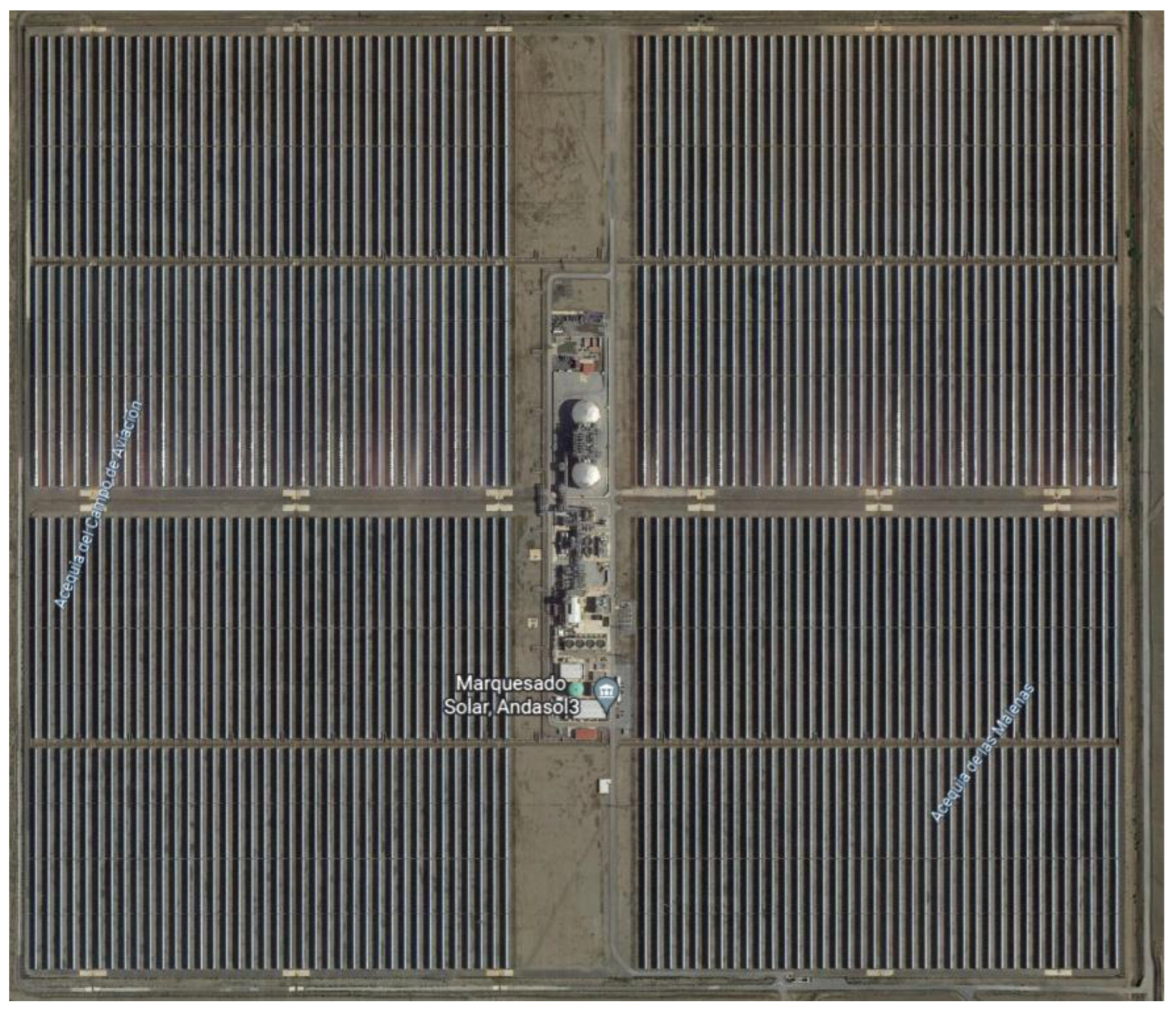
- National Renewable Energy Laboratory, “Andasol 3 CSP Project,” 2021. Available online: https://solarpaces.nrel.gov/project/andasol-3 (accessed on 16 June 2022).
- Instituto Português do Mar e da Atmosfera. Glossário Climatológico/Meteorológico. Available online: https://www.ipma.pt/pt/educativa/glossario/meteorologico/index.jsp?page=glossario_ef.xml&print=true (accessed on 2 August 2021).
- ISO 9060:1990; Solar Energy—Specification and Classifications of Instruments for Measuring Hemispherical Solar and Direct Solar Radiation. International Organization for Standardization: Geneva, Switzerland, 1990. Available online: www.iso.org/standard/16629.html (accessed on 5 December 2020).
- Alami, A.; Conceiç, R.; Gonçalves, H.; Ghennioui, A. CSP Performance and Yield Analysis Including Soiling Measurements for Morocco and Portugal. Renew. Energy 2020, 162, 1777–1792. [Google Scholar] [CrossRef]
- Lopes, D.; Conceição, R.; Gonçalves, H.; Aranzabe, E.; Pérez, G.; Collares-pereira, M. Anti-Soiling Coating Performance Assessment on the Reduction of Soiling Effect in Second-Surface Solar Mirror. Sol. Energy 2019, 194, 478–484. [Google Scholar] [CrossRef]
- ISO 9059:1990; Solar Energy—Calibration of Field Pyrheliometers by Comparison to a Reference Pyrheliometer. International Organization for Standardization: Geneva, Switzerland, 2014. Available online: www.iso.org/standard/16628.html (accessed on 5 December 2020).
- Instituto Português do Mar e da Atmosfera. Rede de Estações Meteorológicas. Available online: https://www.ipma.pt/pt/otempo/obs.superficie/ (accessed on 2 August 2021).
- Instituto Português do Mar e da Atmosfera. Parques Meteorológicos e Equipamentos. Available online: https://www.ipma.pt/pt/educativa/observar.tempo/index.jsp?page=ema.index.xml (accessed on 2 August 2021).
- Long, C.N.; Dutton, E.G. BSRN Global Network Recommended QC Tests, V2.0. Available online: https://bsrn.awi.de/fileadmin/user_upload/bsrn.awi.de/Publications/BSRN_recommended_QC_tests_V2.pdf (accessed on 5 December 2020).
- Kalogirou, S.A. Environmental Characteristics. In Solar Energy Engineering: Processes and Systems; Elsevier: Amsterdam, The Netherlands, 2014; pp. 51–92. [Google Scholar]
- Lopes, F.M.; Silva, H.G.; Salgado, R.; Cavaco, A.; Canhoto, P.; Collares-Pereira, M. Short-Term Forecasts of GHI and DNI for Solar Energy Systems Operation: Assessment of the ECMWF Integrated Forecasting System in Southern Portugal. Sol. Energy 2018, 170, 14–30. [Google Scholar] [CrossRef]
- Finkelstein, J.M.; Schafer, R.E. Improved Goodness-of-Fit Tests. Biometrika 1971, 58, 641–645. [Google Scholar] [CrossRef]
- Lopes, F.M.; Conceição, R.; Fasquelle, T.; Silva, H.G.; Salgado, R.; Canhoto, P.; Collares-Pereira, M. Predicted Direct Solar Radiation (ECMWF) for Optimized Operational Strategies of Linear Focus Parabolic-Trough Systems. Renew. Energy 2020, 151, 378–391. [Google Scholar] [CrossRef]
- Instituto Português do Mar e da Atmosfera. Clima de Portugal Continental. Available online: https://www.ipma.pt/pt/educativa/tempo.clima/ (accessed on 3 August 2021).
- Cavaco, A.; Silva, H.; Canhoto, P.; Neves, S.; Neto, J.; Pereira, M.C. Global Solar Radiation in Portugal and its variability, monthly and yearly. In WES 2016—Workshop on Earth Sciences, Institute of Earth Sciences. 2016, pp. 1–4. Available online: https://dspace.uevora.pt/rdpc/bitstream/10174/19395/1/Afonso_Cavaco_et_al_WES_2016_paper_28.pdf (accessed on 3 August 2021).
- Cunha, L. A Beira Interior—Portugal: Caracterização Física. Rota da Lã Translana Percursos e Marcas um Territ. Front. Beira Inter. (Portugal), Comarc. Tajo-Salor-Almonte 2008. pp. 47–53. Available online: https://www.researchgate.net/publication/324089073_A_beira_Interior_-_Portugal_caracterizacao_fisica (accessed on 3 August 2021).
- Governo Português. Roteiro para a Neutralidade Carbónica 2050. 2019. Available online: https://www.portugal.gov.pt/download-ficheiros/ficheiro.aspx?v=%3D%3DBAAAAB%2BLCAAAAAAABACzMDexAAAut9emBAAAAA%3D%3D.Governo (accessed on 3 August 2021).
- Redes Energéticas Nacionais. DADOS TÉCNICOS. 2021. Available online: https://datahub.ren.pt/media/hkkdskwq/dados-t%C3%A9cnicos-2021.pdf (accessed on 3 August 2021).
- Lopes, T.; Fasquelle, T.; Silva, H.G.; Schmitz, K. HPS2—Demonstration of Molten-Salt in Parabolic Trough Plants—Simulation Results from System Advisor Model. AIP Conf. Proc. 2020, 2303, 110003. [Google Scholar] [CrossRef]


| 2016 | 2017 | 2018 | 2019 | |||||
|---|---|---|---|---|---|---|---|---|
| Error metrics | MOD1 | MOD2 | MOD1 | MOD2 | MOD1 | MOD2 | MOD1 | MOD2 |
| r (---) | 0.97 | 0.98 | 0.97 | 0.98 | 0.97 | 0.98 | 0.97 | 0.98 |
| R2 (---) | 0.94 | 0.95 | 0.95 | 0.96 | 0.94 | 0.96 | 0.95 | 0.96 |
| RMSE (W/m2) | 92.93 | 76.33 | 83.45 | 66.02 | 93.73 | 70.45 | 87.39 | 66.06 |
| MBE (W/m2) | −39.36 | −15.41 | −31.63 | −3.45 | −36.06 | −2.58 | −36.69 | 0.96 |
| MAE (W/m2) | 61.15 | 50.24 | 55.26 | 47.07 | 59.88 | 47.85 | 55.62 | 44.71 |
| 2016 | 2017 | 2018 | 2019 | |||||
|---|---|---|---|---|---|---|---|---|
| Error metrics | Obs. | MOD2 | Obs. | MOD2 | Obs. | MOD2 | Obs. | MOD2 |
| Mean (W/m2) | 512.91 | 528.32 | 549.79 | 553.24 | 462.58 | 465.16 | 531.38 | 530.42 |
| Median (W/m2) | 585.44 | 608.17 | 640.62 | 651.76 | 490.28 | 492.01 | 608.71 | 618.10 |
| σ (W/m2) | 340.88 | 340.48 | 336.46 | 324.92 | 341.51 | 332.86 | 345.34 | 337.18 |
| Eb (kWh/m2/year) | 2074.36 | 2135.19 | 2220.84 | 2234.65 | 1862.85 | 1871.18 | 2149.16 | 2144.13 |
| ΔEb (%) | 2.93 | 0.62 | 0.45 | 0.23 | ||||
| Parameters | Predictor | Present Study | Literature |
|---|---|---|---|
| C | - | −0.0861 | −0.0097 |
| β0 | - | −3.7884 | −5.0317 |
| β1 | kt | 6.8001 | 8.5084 |
| β2 | AST | 0.0050 | 0.0132 |
| β3 | Z | −0.0003 | 0.0074 |
| β4 | Δktc | −1.9639 | −3.0329 |
| β5 | ke | 0.0543 | 0.5640 |
| Station Names | Eb (kWh/m2/year) | Eg (kWh/m2/year) | CF (%) |
|---|---|---|---|
| Sagres | 2245.30 | 1988.94 | 35.2 |
| Faro | 2280.66 | 1963.54 | 36.2 |
| Sines | 2024.39 | 1854.89 | 31.9 |
| Beja | 2145.45 | 1878.65 | 31.8 |
| Évora | 2030.14 | 1808.25 | 30.3 |
| Lisboa/Geofísico | 1888.81 | 1755.44 | 29.1 |
| Lisboa/Gago Coutinho | 1985.18 | 1788.31 | 30.1 |
| Portalegre | 1875.37 | 1698.47 | 27.4 |
| Cabo Carvoeiro | 1521.87 | 1625.36 | 22.8 |
| Castelo Branco | 2078.07 | 1769.59 | 31.2 |
| Coimbra | 1809.43 | 1645.21 | 25.7 |
| Penhas Douradas | 1467.85 | 1672.30 | 19.4 |
| Viseu | 1786.90 | 1622.90 | 26.1 |
| Porto | 1624.47 | 1603.49 | 24.2 |
| Vila Real | 1603.01 | 1561.46 | 23.6 |
| Bragança | 1847.01 | 1648.14 | 28.3 |
Publisher’s Note: MDPI stays neutral with regard to jurisdictional claims in published maps and institutional affiliations. |
© 2022 by the authors. Licensee MDPI, Basel, Switzerland. This article is an open access article distributed under the terms and conditions of the Creative Commons Attribution (CC BY) license (https://creativecommons.org/licenses/by/4.0/).
Share and Cite
Tavares, A.M.; Conceição, R.; Lopes, F.M.; Silva, H.G. Development of a Simple Methodology Using Meteorological Data to Evaluate Concentrating Solar Power Production Capacity. Energies 2022, 15, 7693. https://doi.org/10.3390/en15207693
Tavares AM, Conceição R, Lopes FM, Silva HG. Development of a Simple Methodology Using Meteorological Data to Evaluate Concentrating Solar Power Production Capacity. Energies. 2022; 15(20):7693. https://doi.org/10.3390/en15207693
Chicago/Turabian StyleTavares, Ailton M., Ricardo Conceição, Francisco M. Lopes, and Hugo G. Silva. 2022. "Development of a Simple Methodology Using Meteorological Data to Evaluate Concentrating Solar Power Production Capacity" Energies 15, no. 20: 7693. https://doi.org/10.3390/en15207693
APA StyleTavares, A. M., Conceição, R., Lopes, F. M., & Silva, H. G. (2022). Development of a Simple Methodology Using Meteorological Data to Evaluate Concentrating Solar Power Production Capacity. Energies, 15(20), 7693. https://doi.org/10.3390/en15207693