Article

Modeling of Thermal-Lag Engine with Validation by Experimental Data

Department of Aeronautics and Astronautics, National Cheng Kung University, No.1, University Road, Tainan 70101, Taiwan
*
Author to whom correspondence should be addressed.
Energies 2022, 15(20), 7688; https://doi.org/10.3390/en15207688
Submission received: 14 September 2022 / Revised: 7 October 2022 / Accepted: 14 October 2022 / Published: 18 October 2022
(This article belongs to the Section I: Energy Fundamentals and Conversion)

Abstract

:
Thermal-lag engines are external combustion engines with a single moving piston. This feature leads to lower manufacturing and maintenance costs than traditional Stirling engines. Although the original concept of thermal-lag engines was invented roughly 35 years ago, the information on thermal-lag engines is still limited. Therefore, this study focuses on thermal-lag engine performance by developing a three-dimensional computational fluid dynamics (CFD) model. The grid independence check and the time step independence check are firstly performed to select the number of elements and size of the time step for simulation. The CFD model is then validated by the experimental data, which were collected by measuring an existing prototype engine. It has been found that the CFD predictions are well fitted to the experimental data over the range of engine speed from 200 to 1600 rpm at temperatures of 1173 or 1273 K. Furthermore, the CFD model predicts that the maximum engine power is 21.1 W while the prototype engine practically generates the highest power of 22.35 W at 1000 rpm and 1273 K. Finally, a further parametric study shows that crank radius, piston diameter, working gas mass, working gas species, and heating temperature significantly affect engine power.

1. Introduction

Thermal-lag engines are one kind of external combustion engine in which working gas is periodically cooled down and heated up between hot and cold thermal reservoirs to generate mechanical energy. Thermal-lag engines and Stirling engines, therefore, have several advantages in common, for example, the possibility to harness many kinds of heat energy [1,2], produce a low level of noise, emit low pollutants, operate safely, and have the self-starting ability [3,4]. In particular, a thermal-lag engine structurally consists of only one moving piston, whereas traditional Stirling engines possess at least two moving parts. This distinct feature of thermal-lag engines offers great promise of lower manufacturing and maintenance costs as compared to traditional Stirling engines [5].
Chen and West [6] proposed the thermal-lag engine concept in 1987. Tailer [7] built the first thermal-lag engine, in which imperfect heat transfer between the wall and working gas was found to cause the phase difference between the piston position and the gas temperature. Wicks et al. [8] put forward the very first numerical model of Tailer’s thermal-lag engine. Arques [9] introduced pressure loss into the numerical analysis of the Wicks-Tailer cycle. It was shown that the P-V diagram is much narrower than that of a traditional Stirling engine. Altamirano et al. [10] used two control volumes to analyze Organ’s thermal-lag engine performance. The study suggested that a good design should have the largest possible surface of the hot chamber but an optimal area of the cold chamber. Cheng and Yang [11] numerically considered the thermodynamic behaviors of the thermal-lag engine. The temperature distribution along the regenerative heater was derived in terms of its wall temperature features while the temperature in the hot and cold chambers was solved from the energy equations. The engine power can achieve 17.35 W at 600 rpm and 19.62 W at a volume of 14.2 cm3. The smaller the buffer-chamber volume, the higher the engine performance. Furthermore, the maximum power can be achieved with optimal bore diameter. Later, Cheng, et al. [12] exploited the thermodynamic-dynamic model to study the dynamic behaviors of thermal-lag engines. The numerical model can predict some possible operational modes, namely, swinging-to-decaying mode, rotating mode, swinging-to-rotating mode, and swinging mode. The study showed that the undesired swinging mode can be observed if the bore size and thermal resistance are too large. Effects of bore size, stroke, and gas-chamber volume on engine performance were also pointed out. Yang and Cheng [13] analytically solved a thermal-lag engine mathematical model for oscillation amplitude and thermal-lag phase angle. In particular, startable and unstartable zones in the influential parameter space were demonstrated from the analytical solution of the amplitude. Lately, Yang and Cheng [14] developed analytical solutions to a nonlinear dimensionless dynamic model. The results showed that the larger the spring stiffness, volume of the cold chamber, and loading are, the more difficult it is to start the engine. Recently, Alborzi et al. [15] used the genetic algorithm and the neural network to raise the thermal-lag engine power to 86.9% from the baseline case. ElDebawy et al. [16] developed a 3D CFD model of a thermal-lag engine. In their study, it was shown that the indicated power is 0.218 W at 3.2 Hz and 0.3385 W at 5 Hz. The obtained CFD results are close to the experimental data; however, the engine power is too low for practical applications. The effects of dwell time and swirling motion were also studied. Most recently, Yang et al. [17] solved a dynamic model of a thermal-lag Stirling engine linked to a flywheel by the multiple-scale method. The solution showed that there are three operating modes: swinging, rotating, and decaying. The transition behavior between these modes was well discussed. The authors found seven operating regions in the plane of the dimensionless frequency and the dimensionless temperature.
There have been several possible methods of modeling thermal-lag engines. The analytical method gives exact solutions or power series solutions [5,13,14,17]. On the other hand, the thermodynamic-model methods [11,12,18,19,20] have also been built, based on dominant longitudinal variations of temperature and velocity fields. This kind of method is mathematically simple and, consequently, requires less computational effort and computer storage. This feature enables the thermodynamic-model method to apply to the quick evaluation of thermal efficiency, dynamic behaviors, and even engine optimization. In contrast, CFD analyses [16,21,22,23] may take many cycles to get the final engine speed, but they can improve the solution accuracy and generate more complete pictures of the transient 3D temperature and velocity fields. Therefore, the CFD-model method is a more complete model of engines and is expected to deliver more accurate solutions than the aforementioned analytical or thermodynamic-model methods.
As a matter of fact, in 2014, Lin [24] built a prototype thermal-lag engine in the Power Engine and Clean Energy Laboratory (PEACE Lab.), NCKU. The authors found that the engine could be self-started and then practically generated the highest power of 22.35 W at 1000 rpm and 1273 K. Be aware that this prototype thermal-lag engine simply used air at 1 bar as the working gas; one can expect that the engine may achieve higher power if the parameters could be properly selected. Unfortunately, deeper insight into the physical phenomena in this thermal-lag engine could not be obtained simply based on the experimental data. Therefore, the subtle influence of imperfect heat transfer on power generation and thermal efficiency has not been sufficiently investigated.
From the literature review above, most of the existing studies utilized the analytical or thermodynamic-model methods to study thermal-lag engine performance. To the best of the authors’ knowledge, the report of ElDebawy et al. [16] is the only three-dimensional CFD study of the thermal-lag engine. However, as has been mentioned earlier, the power output of their engine, roughly between 0.2 and 0.34 W, is too low for practical applications. Under these circumstances, this study is focused on the development of a complete three-dimensional CFD model that applies the analysis of thermal-lag engine performance. Furthermore, the model will be validated based on the experiments with the prototype engine developed by Lin [24] to ensure the feasibility of the model.

2. Computational Fluid Dynamics Model

2.1. Configuration of Thermal-Lag Engine

Figure 1a,b show the schematic diagram and prototype engine, respectively. The whole space in the engine includes six main chambers: compression chamber, inner cylinder, heater head, heater fins, regenerator, and cooler fins. The walls of the heater fins and the heater head are subjected to the heating temperature T h where the thermal energy is absorbed from the hot reservoir. Meanwhile, the walls of the compression chamber and the cooler fins are maintained at the cooling temperature T c where part of the heat is released to the surroundings. A single piston displaces the working gas in the compression chamber. Thus, the thermal-lag engine is also called the ‘one-piston’ engine. In Figure 1a, the double-headed arrows represent the periodic flow directions inside the whole space. Figure 1b shows the photograph of the prototype thermal-lag engine developed by Lin [24]. The heating is provided by using an electrical heater or a torch with which the heating temperature can be adjusted for experiments. The heater head and the heater fins are made to serve as the heater heat exchanger. The 4 ports shown in Figure 1b are the 2 inlets and 2 exits of the cooling water flowing through the liquid cooler. The cooling water helps cool down the wall temperature of the compression chamber and the cooler fins. The cooler fins are used to enhance the heat transfer to the working gas. The engine specifications are provided in Table 1. Here in this study, the specifications of this engine are chosen to be the baseline case such that the comparison between numerical predictions and experimental data is possible. It is noted that the prototype engine uses air as the working gas.

2.2. Governing Equations

The following assumptions are added to the mathematical model:
  • The working gas equation of state is ideal;
  • The gravity effect on the flow and thermal fields is neglected;
  • Local thermal equilibrium in the regenerator is assumed.
The mathematical model involves a set of governing transport equations for the working gas solution domain as follows:
Continuity equation:
ρ t + ρ u i x i = 0
Momentum equations:
ρ u i t + ( ρ u j u i + P δ i j ) x j = ( τ j i + τ j i R ) x j
where Reynolds stress components τ i j R are expressed in terms of mean velocity components as
τ i j R = ρ u i u j ¯ = μ t ( u i x j + u j x i ) 2 3 ( ρ k + μ t u k x k ) δ i j
Energy equation:
ρ e t + x i ρ u i ( E + P ρ ) = x i ( k e f f T x i + τ i j R u j )
where k e f f is the effective thermal conductivity which is determined with
k e f f = k m o l + c p μ t P r t
and k m o l is the molecular thermal conductivity.
Equation of state:
P = ρ R T
Energy equation in the regenerator:
( γ ρ e + ( 1 γ ) ρ s e s ) t + ( ρ e + p ) u = ( k e f f T i h i J i + τ u )
The loss in momentum S must be added to Equation (2) to take into account the effect of the regenerator on the momentum.
S = μ D u C ρ 2 | u | u
The regenerator wire mesh is made of stainless steel and has a total mass of 4.5 g and a wire diameter of 0.025 mm. From this information, the calculation of two coefficients D and C is mentioned in [25].
Because the engine geometry is complex and the range of engine speed is varied from 200 to 1600 rpm, it is expected that turbulent flow prevails in the working space. The turbulent flow increases the transport and mixing of heat, mass, and momentum in the working space. In this study, the realizable k ϵ model is opted for the turbulent fields because of its efficiency in computational time and reasonable accuracy through the mathematical constraints on turbulent viscosity coefficient C μ and the fact that the ϵ -equation was obtained from the exact mean-square vorticity fluctuation equation [26]. The model consists of the following equations:
k -equation:
ρ k t + ρ u i k x i = ( μ + μ t σ k ) k + G k + G b ρ ϵ Y M + S k
ϵ-equation:
ρ ϵ t + ρ u i ϵ x i = ( μ + μ t σ ϵ ) ϵ + ρ C 1 S ϵ ρ C 2 ϵ 2 k + ν ϵ + C 1 ϵ ϵ k C 3 ϵ G b + S ϵ
Eddy viscosity is modeled in terms of k and ϵ
μ t = C μ ρ k 2 ϵ
In this study, the molecular dynamic viscosity and thermal conductivity are determined from the expression proposed by Kuehl [27].
f ( T , p ) = a 0 + a 1 T + a 2 T 2 + a 3 T 3 + a 4 p + a 5 + a 6 p + a 7 p 2 T T c r i t
Values of these properties are estimated at the temperature ( T h + T c ) / 2 .
From the numerical predictions of varying volume-averaged pressure, the power is computed by the following expression
W ˙ = ω 60 c y c l e P c d V c
where ω is the engine speed in rpm.

2.3. Initial-Boundary Conditions

Table 2 conveys the boundary and initial conditions for the baseline simulation case. The no-slip condition is adopted for the momentum equation on all the solid walls, and thus the velocity of the working gas on the piston surface must be equal to that of the moving piston. The piston velocity is a function of the crank radius r , connecting-rod length L, angular velocity ω, and crank angle θ .
v p = ω π 30 r c o s θ ( 1 + s i n θ ( L r ) 2 c o s 2 θ )
where the crank angle θ = ω π t / 30 π / 2 . In this study, the unit of ω is rpm.
In the CFD model, the dynamic mesh is performed by the layering method [26], which provides a method for adding or deleting the cell layer next to the moving boundary based on the height of the layer. The couple algorithm is selected to resolve the pressure-velocity coupling because it is necessary for all transient problems with large time steps. Table 3 summarizes the spatial–temporal discretization schemes.

3. Preliminary Numerical Checks

Both the grid independence and the time step independence checks are indispensable preliminary checks with any CFD analysis and hence, they are discussed in detail in this section. Once the preliminary numerical checks are completed, a parametric study of the effects of several influential geometrical and operational parameters on the power of the engine will then be performed. In this study, the CFD model is run on the ANSYS Fluent 18.0 platform [26] installed in an HP Z6 G4 workstation with Intel® Xeon® Silver 4110 CPU@ 2.10 GHz.

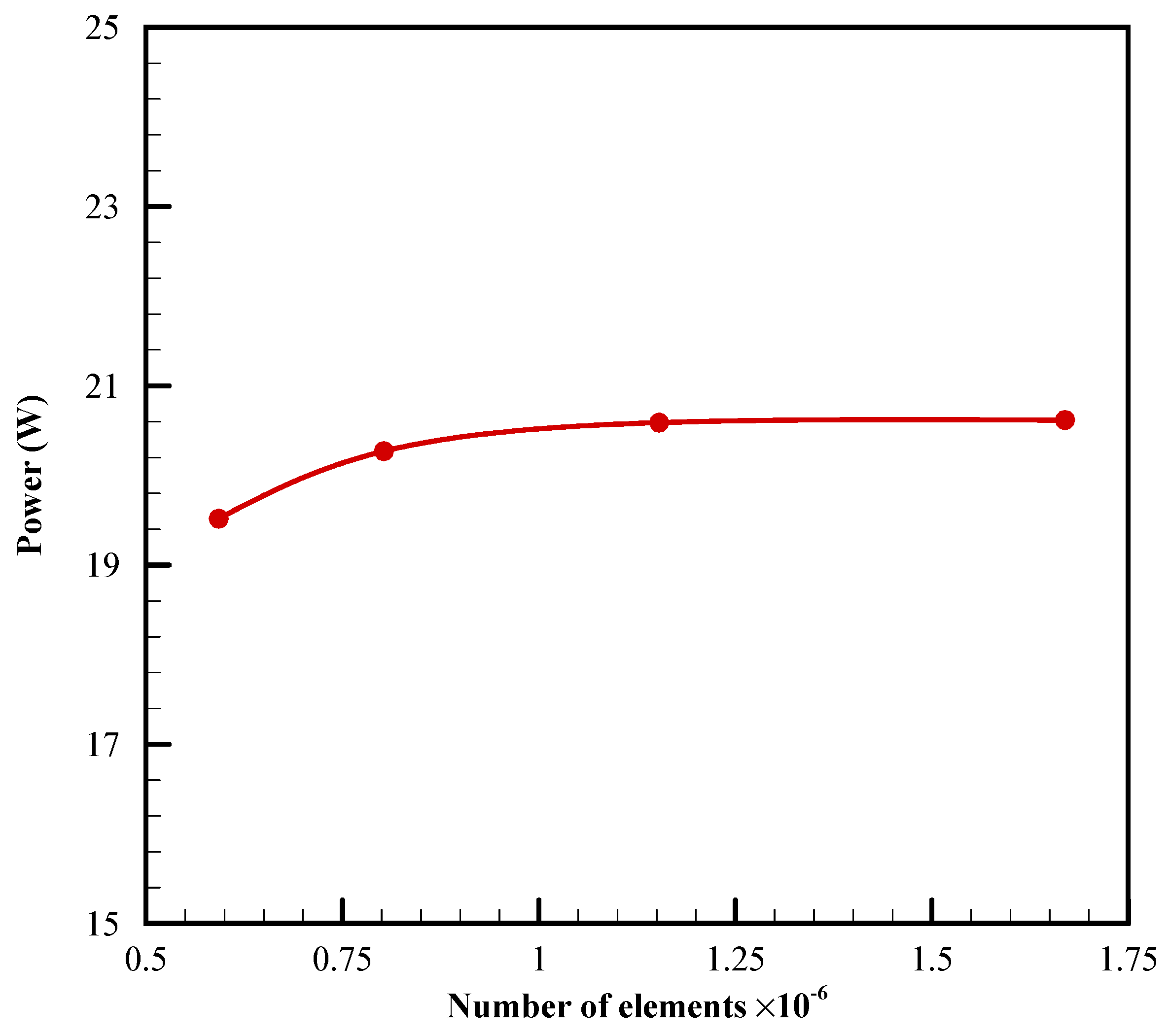
3.1. Grid Independence Check

The CFD analysis requires the grid independence check to make sure the numerical solution converges on a sequence of decreasing mesh sizes [28]. To do so, a set of four grids with 592,591, 802,765, 1,153,154, and 1,669,431 elements are generated. Figure 2 indicates that, for the baseline case, the predicted value of the engine power goes up and then converges as the number of elements increases further. Particularly, the difference in power between the two latter meshes is only within 0.1 W. For the trade-off between computation time and accuracy, the grid with 1,153,154 elements is an appropriate choice for the remaining simulation cases.

3.2. Time Step Independence Check

In a transient problem, the time step independence check is also required to guarantee that the selected time step size is good enough to approximate the solutions for the governing equations. Here, the mesh is fixed at 1,153,154 elements, while four time steps of 4.6875 × 10⁻⁴, 4.17 × 10⁻⁴, 3.75 × 10⁻⁴, and 3.125 × 10⁻⁴ s are tested in the simulation of the baseline case. The results are displayed in Figure 3. It is seen that all four time step cases result in relative differences smaller than 0.1 W in the values of powers. Therefore, typically a time-step size of 3.75 × 10⁻⁴ s is used for the CFD simulations.

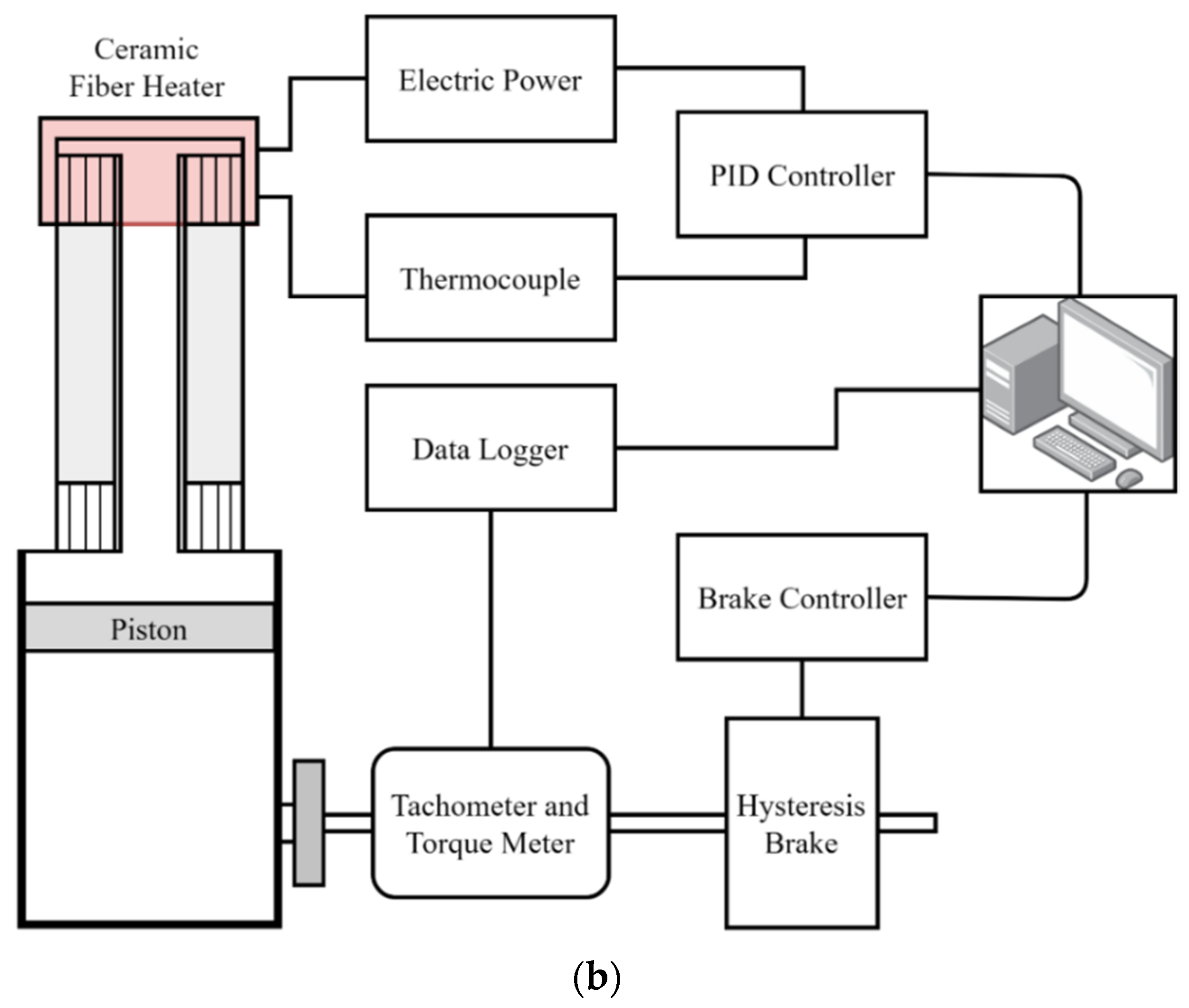
4. Experimental System

Figure 4 shows briefly the experimental system and its schematic used by Lin [24]. A ceramic fiber heater consisting of an array of helical alloy wires can produce the heating temperature. This heater enables thermal energy to be generated uniformly inside the device. K-type thermocouples are employed to measure the temperatures inside the ceramic fiber heater. The thermal energy generation as well as the heating temperature is adjusted by a PID temperature controller to which the thermocouple is connected. In addition, a hysteresis brake is applied on the engine shaft. The engine rotation speed and the applied torque are measured by the tachometer and torque sensor, respectively. The data are all recorded by the data logger and transferred to a personal computer for further processing.
The accuracy of K-type thermocouples is ±0.75%. The uncertainty of the thermostat using a PID controller is within ±1 K. The sensor measuring the charged pressure has an accuracy of 1.5%.

5. Results and Discussion

Figure 5 shows results from the CFD model and experiment at two temperature levels 1173 and 1273 K over the engine speed from 200 to 1600 rpm. In this figure, it is seen that at 1173 K the discrepancy between numerical and experimental data is appreciable at low engine speed. The CFD model overestimates the power at lower rotation speeds while it underestimates the power at higher rotation speeds. The reason behind the discrepancy may come from the fact that the thermal conductivity is overestimated at low engine speeds and underestimated at high engine speeds when its value is computed at the arithmetic average of heating and cooling temperatures, as mentioned in Section 2.2. Nonetheless, the trends of the two sets of data are still similar. At the temperature level of 1273 K, the CFD and experimental results are in close agreement over the whole range of the rotation speed. In the case of 1273 K, the CFD model predicts that the maximum power is reached at around 1000 rpm and this result is confirmed by the experimental data. Moreover, the numerical prediction of the maximum engine power is 21.1 W, and the measured maximum power is 22.35 W. The difference is only 1.25 W. This implies that the CFD model can lead to accurate results for cases with high heating temperatures. However, the error of the numerical predictions will be larger if the heating temperature is lowered. Note that from the experimental data, the current design produces high power at high heating temperatures. In contrast, its power becomes impractical with heating temperatures below 700 K. This raises the demand for modifying the current design to get higher power at a lower temperature.
Several snapshots of the periodic thermal and flow fields for the baseline case, with a grid of 1,153,154 elements and a time step of 3.75 × 10⁻⁴ s, are shown in Figure 6 and Figure 7, respectively. The expansion process corresponds to the sequence of instants (b)-(c)-(d), which is associated with the downward motion of the piston. Consequently, the hot jet from the hot region continuously pours into the compression chamber and maintains a highly non-uniform temperature field in the compression chamber. The impingement of the hot jet onto the piston surface produces strong vortices in the compression chamber, as seen clearly in Figure 6c and Figure 7c. It is noted that the pair of vortices plays a twofold role in heat transfer. On one hand, it circulates the hot flow close to the wall and forms a strong gradient near the wall. This effect enhances the heat transfer in the cold region. On the other hand, the pair of vortices enforces the mixing between the entering hot gas and the cold gas; therefore, the temperature field in the compression chamber becomes uniform.
The process (d)-(a)-(b) is the compression process as the piston moves upwards. As the piston is around the bottom dead center (BDC), the hot jet still impinges on the piston surface for a short time, as shown in Figure 6d. However, as the piston starts to move upwards, the upward motion of the piston then pushes the cold working gas to move from the compression chamber, through the cylinder, heater head, heater fins, and regenerator, and then reaches the cooler fins chamber. The compression-chamber temperature becomes almost uniform at the end of the compression process, as shown in Figure 6b. Additionally, the flow is stagnant at the bottom of the cooler fins zone. Consequently, the cooler-fin temperature field is almost maintained at the cold temperature. The CFD results also exhibit that a linear temperature profile in the vertical direction can be established between the heater fins and the cooler fins chambers during an entire cycle, as clearly seen in Figure 6. Furthermore, the heater head strengthens the heat transfer process during the compression process while it enhances the mixing process inside the hot jet flow due to high flow velocity through the small gap, as shown in Figure 7a,c.
Next, variations of engine power under the effects of some influential operational and geometrical parameters are evaluated by the present CFD model. The crank radius is regarded as one of the influential parameters of engine power. The range of crank radius under investigation is from 20 mm to 30 mm. The power rises approximately linearly from 14.3 up to 28.5 W with the crank radius, as plotted in Figure 8, because the larger the crank radius, the larger the swept volume and, in turn, the larger the compression ratio. Consequently, the increase in the compression ratio expands the variation range of pressure and thus increases the power, as was also found by Chen, Yang, and Salazar [29].
Additionally, a larger diameter of the piston sweeps more of the working gas mass and leads to a higher compression ratio. The piston diameter is expected to have a positive effect on the engine power. Indeed, the power is elevated from 18.7 to 21.6 W as the piston diameter is increased from 56 mm to 68 mm, as shown in Figure 9.
The influence of the mass of working gas relative to that of the baseline case m b a s e on the engine power is further illustrated in Figure 10. Engine power rises from 20.6 W to 46.8 W as the mass ratio m / m b a s e increases from 1.0 to 3.0. This approximately linear relationship between the engine power and the total working gas mass can be explained by the linear relationship between the working mass and the engine power, as discussed in [30]. However, since the mass flow rate through the regenerator increases with the total mass, the dominant pressure loss gradually switches from the viscous term with the first order of the low velocity to the inertial term with the second order of the high velocity. The two terms can be observed from the momentum sink term S in Equation (8). Consequently, the larger the total mass, the greater the deviation of the engine power from the linear dashed curve in Figure 10.
Furthermore, the change in power due to the use of other gases can be interesting to the related researchers. For example, Katooli et al. [31] showed the gamma-type Stirling engine with hydrogen delivered the highest output work among helium, hydrogen, and nitrogen. Cheng et al. [32] found that, for the low temperature differential gamma-type Stirling engine, helium, and hydrogen generated approximately equal powers, while air and nitrogen gave the lowest powers. Erol and Çalışkan [33] also investigated a rhombic-drive β-type Stirling engine using different working gases, including air, argon, carbon dioxide, helium, and nitrogen. The authors found that helium generally gave the highest power for all engine speeds and charged pressures.
Therefore, even though the working gas of the prototype engine uses air, in the present simulation the relative performance of helium, hydrogen, and air are compared. It is noted that the boundary and initial conditions of these simulation cases are the same as those in Table 2. Figure 11 provides the results of engine power corresponding to the three respective gases. It is seen that for the particular case, the engine powers using air, helium, and hydrogen are 20.6, 27.4, and 30.1 W, respectively. This implies that changing the gas is possible to significantly improve the power of the engine. The engine power is proportional to the heat transfer rate absorbed in the hot chamber. Because hydrogen has the highest thermal conductivity while air has the lowest, this probably partially explains why the highest engine power is produced with hydrogen and the lowest is with air. However, since hydrogen is highly flammable, it is not recommended to be the working gas, despite the power. Alternatively, helium is recommended since it is not flammable and the relative difference in power between helium and hydrogen is only within 10%.
Figure 12 depicts the variation of the engine power with the heating temperature at the engine speed of 800 rpm. As illustrated in this figure, the engine power is increased from 13.6 to 20.6 W at 973 and 1273 K, respectively. An increase in the heating temperature improves the difference in temperature between the cold and hot chambers and then results in a growth in engine power. It is noted that the melting points of materials, the lifespan of the engine, and the temperature of heat sources are factors that limit the heating temperature.

6. Conclusions

This study firstly proposes a 3D CFD model, which is more accurate in predictions of the thermal-lag engine performance than the existing thermodynamic models. The most important thing is that the CFD model is validated by experiments. The value of this paper is that it proposes the first validated CFD model of a thermal-lag engine whose power is higher than 20 W. Other remarkable conclusions reached in the study are:
  • The CFD results are remarkably close to the experimental data over the wide range of engine speeds from 200 to 1600 rpm at the temperature of 1273 K. The experiments show that the maximum power of 22.35 W can be reached at 1273 K and 1000 rpm, and the CFD model prediction is 21.1 W. However, the error of the numerical predictions will be larger if the heating temperature is lowered. Furthermore, from the experimental data, the current design produces high power at high heating temperatures. In contrast, its power becomes impractical with heating temperatures below 700 K. This raises the demand for modifying the current design to get higher power at a lower temperature.
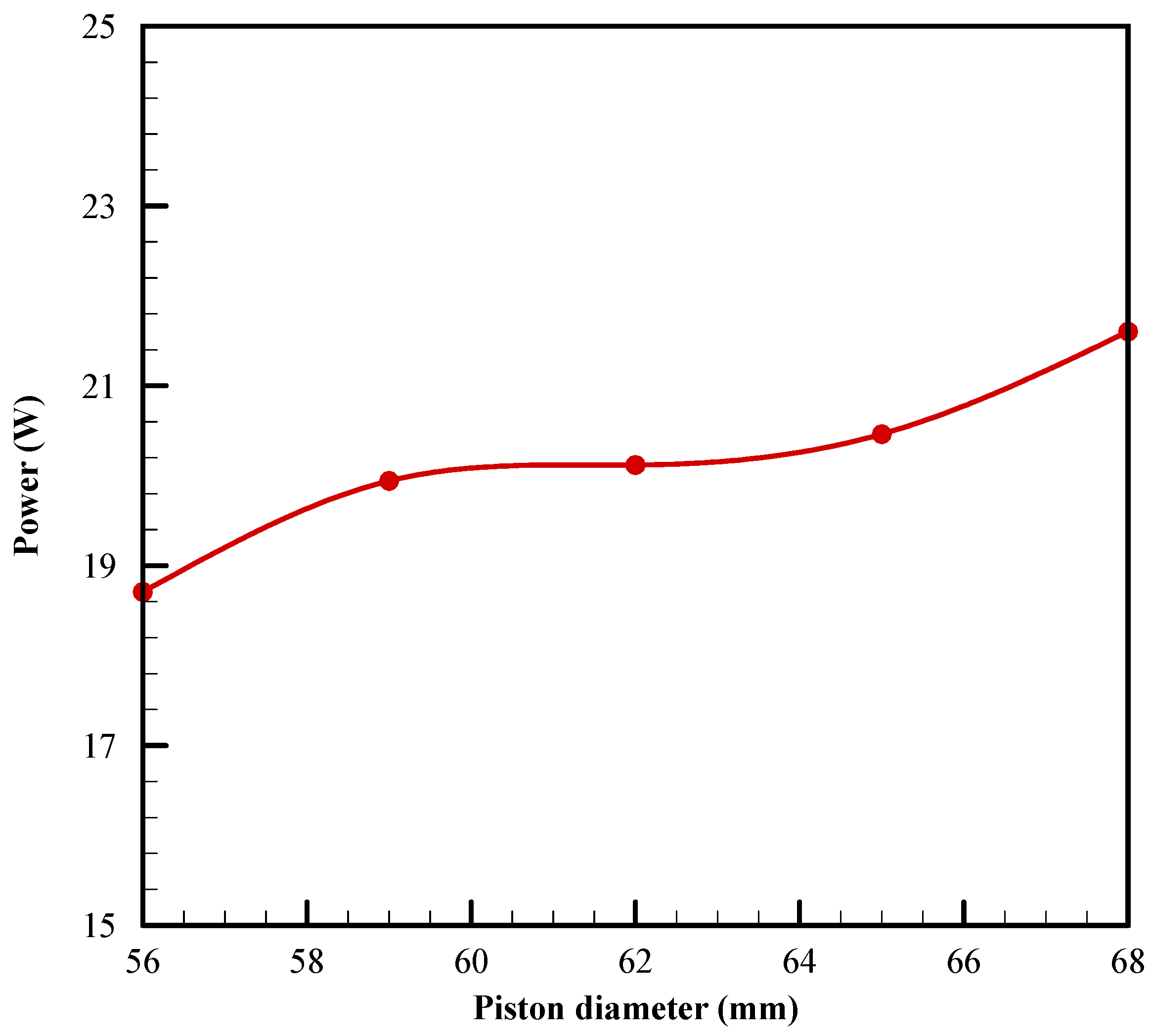
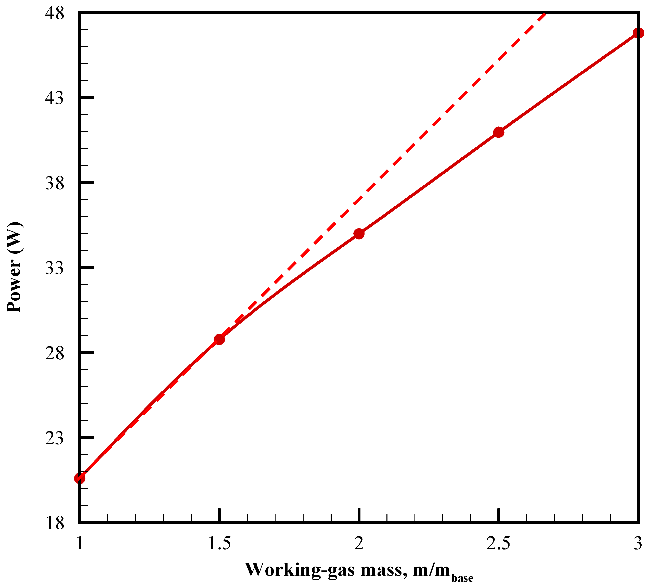
  • The effects of the influential geometrical and operational parameters on the power of the engine are evaluated by the present CFD model. The parametric study shows that the crank radius, the piston diameter, the working gas mass, and the heating temperature significantly affect the engine power. It is found that as the crank radius is increased from 20 mm to 30 mm, the power rises approximately linearly from 14.3 to 28.5 W. As the piston diameter varies from 56 mm to 68 mm, the engine power rises from 18.7 W to 21.6 W. Meanwhile, it is found that the mass of the working gas has a strong effect on the engine power. As the mass ratio increases from 1 to 3.0, the engine power grows approximately linearly from 20.6 W to 46.8 W. In this study, the engine power is elevated from 13.6 to 20.6 W at 973 and 1273 K, respectively.
  • Based on the obtained results regarding the dependence of engine power on the working gases used, it is seen that changing the gas is possible to significantly enhance the power of the engine. Results show that the highest engine power is generated with hydrogen and the lowest is with air. However, since hydrogen is highly flammable, it is not recommended to be the working gas, despite the power. Alternatively, helium is recommended since it is not flammable and the relative difference in power between helium and hydrogen is only within 10%.
However, note that this study is limited to thermo-fluidic analysis of the thermal-lag engine performance based on a 3D CFD model. Since a real engine operates based on the interaction between the working gas thermo-fluidic behaviors and the mechanism dynamic behaviors, a thorough analysis should be conducted in the future by incorporating the dynamic model with the thermo-fluidic model.

Author Contributions

Conceptualization, C.-H.C.; data curation, D.-T.P.; formal analysis, C.-H.C.; investigation, D.-T.P.; resources, C.-H.C.; software, D.-T.P.; supervision, C.-H.C.; writing—original draft, D.-T.P.; writing—review and editing, C.-H.C. All authors have read and agreed to the published version of the manuscript.

Funding

This research received no external funding.

Data Availability Statement

No other data is available.

Conflicts of Interest

The authors declare no conflict of interest.

References

  1. Breeze, P. Stirling Engines and Free Piston Engines. In Piston Engine-Based Power Plants; Elsevier: Amsterdam, The Netherlands, 2018; pp. 59–70. [Google Scholar] [CrossRef]
  2. Islam, M.; Hasanuzzaman, M.; Pandey, A.; Rahim, N. Modern energy conversion technologies. In Energy for Sustainable Development: Demand, Supply, Conversion and Management; Hasanuzzaman, M., Rahim, N.A., Eds.; Elsevier: Amsterdam, The Netherlands, 2020; pp. 19–39. [Google Scholar]
  3. Varbanov, P.; Klemeš, J. Small and micro combined heat and power (CHP) systems for the food and beverage processing industries. In Small and Micro Combined Heat and Power (CHP) Systems: Advanced Design, Performance, Materials and Applications; Beith, R., Ed.; Elsevier: Amsterdam, The Netherlands, 2011; pp. 395–426. [Google Scholar]
  4. Nagaoka, Y.; Nakamura, M.; Yamashita, K.; Ito, Y.; Haramura, S.; Yamaguchi, K. Development of Stirling Engine Heat Pump. In Heat Pumps: Solving Energy and Environmental Challenges; Saito, T., Ed.; Elsevier: Amsterdam, The Netherlands, 1990; pp. 595–603. [Google Scholar]
  5. Yang, H.-S.; Cheng, C.-H. A nonlinear non-dimensional dynamic model for free piston thermal-lag Stirling engine. Energy Procedia 2014, 61, 2662–2665. [Google Scholar] [CrossRef] [Green Version]
  6. Chen, N.; West, C. A single-cylinder valveless heat engine. In Proceedings of the 22nd Intersociety Energy Conversion Engineering Conference, Philadelphia, PA, USA, 10–14 August 1987; p. 9070. [Google Scholar]
  7. Tailer, P.L. External combustion Otto cycle thermal lag engine. In Proceedings of the 28th Intersociety Energy Conversion Engineering Conference, Atlanta, GA, USA, 8–13 August 1993; pp. 943–947. [Google Scholar]
  8. Wicks, F.; Caminero, C. The Peter Tailer external combustion thermal lag piston/cylinder engine analysis and potential applications. In Proceedings of the 29th Intersociety Energy Conversion Engineering Conference, Monterey, CA, USA, 7–12 August 1994; pp. 951–954. [Google Scholar]
  9. Arques, P. Theoretical and numerical study, improvement of the Wicks-Tailer cycle. In Proceedings of the 30th Intersociety Energy Conversion Engineering Conference, Orlando, FL, USA, 30 July–5 August 1995; pp. 407–412. [Google Scholar]
  10. Altamirano, C.F.-A.; Moldenhauer, S.; Bayón, J.G.; Verhelst, S.; De Paepe, M. A two control volume model for the Thermal Lag Engine. Energy Convers. Manag. 2014, 78, 565–573. [Google Scholar] [CrossRef]
  11. Cheng, C.-H.; Yang, H.-S. Theoretical model for predicting thermodynamic behavior of thermal-lag Stirling engine. Energy 2013, 49, 218–228. [Google Scholar] [CrossRef]
  12. Cheng, C.-H.; Yang, H.-S.; Jhou, B.-Y.; Chen, Y.-C.; Wang, Y.-J. Dynamic simulation of thermal-lag Stirling engines. Appl. Energy 2013, 108, 466–476. [Google Scholar] [CrossRef]
  13. Yang, H.-S.; Cheng, C.-H. Stability analysis of thermal-lag Stirling engines. Appl. Therm. Eng. 2016, 106, 712–720. [Google Scholar] [CrossRef]
  14. Yang, H.-S.; Cheng, C.-H. Theoretical solutions for power output of thermal-lag Stirling engine. Int. J. Heat Mass Transfer 2017, 111, 191–200. [Google Scholar] [CrossRef]
  15. Alborzi, M.; Sarhaddi, F.; Sobhnamayan, F. Optimization of the thermal lag Stirling engine performance. Energy Environ. 2019, 30, 156–175. [Google Scholar] [CrossRef]
  16. ElDebawy, M.; Beshay, K.R.; Fernandez-Aballi, C.; Khalil, E.E. CFD Analyses of Thermal Lag Engine. In Proceedings of the AIAA Propulsion and Energy 2019 Forum, Indiana, IN, USA, 19–22 August 2019; p. 4063. [Google Scholar]
  17. Yang, H.-S.; Cheng, C.-H.; Ali, M.A. Performance and operating modes of a thermal-lag Stirling engine with a flywheel. Appl. Therm. Eng. 2022, 205, 118061. [Google Scholar] [CrossRef]
  18. Cheng, C.-H.; Phung, D.-T. Numerical Optimization of the β-Type Stirling Engine Performance Using the Variable-Step Simplified Conjugate Gradient Method. Energies 2021, 14, 7835. [Google Scholar] [CrossRef]
  19. Udeh, G.T.; Michailos, S.; Ingham, D.; Hughes, K.J.; Ma, L.; Pourkashanian, M. A new non-ideal second order thermal model with additional loss effects for simulating beta Stirling engines. Energy Convers. Manag. 2020, 206, 112493. [Google Scholar] [CrossRef]
  20. Cheng, C.-H.; Tan, Y.-H. Numerical optimization of a four-cylinder double-acting Stirling engine based on non-ideal adiabatic thermodynamic model and scgm method. Energies 2020, 13, 2008. [Google Scholar] [CrossRef] [Green Version]
  21. El-Ghafour, S.; El-Ghandour, M.; Mikhael, N. Three-dimensional computational fluid dynamics simulation of Stirling engine. Energy Convers. Manag. 2019, 180, 533–549. [Google Scholar] [CrossRef]
  22. Ben-Mansour, R.; Abuelyamen, A.; Mokheimer, E.M. CFD analysis of radiation impact on Stirling engine performance. Energy Convers. Manag. 2017, 152, 354–365. [Google Scholar] [CrossRef]
  23. Caetano, B.C.; Lara, I.F.; Borges, M.U.; Sandoval, O.R.; Valle, R.M. A novel methodology on beta-type Stirling engine simulation using CFD. Energy Convers. Manag. 2019, 184, 510–520. [Google Scholar] [CrossRef]
  24. Lin, H.-H. Theoretical Analysis and Optimal Design of a Pulse-Tube Stirling Engine. Master’s Thesis, National Cheng-Kung University, Tainan, Taiwan, 2014. [Google Scholar]
  25. Boroujerdi, A.; Esmaeili, M. Characterization of the frictional losses and heat transfer of oscillatory viscous flow through wire-mesh regenerators. Alex. Eng. J. 2015, 54, 787–794. [Google Scholar] [CrossRef] [Green Version]
  26. ANSYS Inc. ANSYS Fluent Theory Guide: Release 18.0; ANSYS Inc.: Canonsburg, PA, USA, 2017. [Google Scholar]
  27. Kuehl, H. Numerically efficient modelling of non-ideal gases and their transport properties in Stirling cycle simulation. In Proceedings of the 17th International Stirling Engine Conference and Exhibition, Newcastle upon Tyne, UK, 24–26 August 2016; pp. 572–579. [Google Scholar]
  28. Toro, E.F. Riemann Solvers and Numerical Methods for Fluid Dynamics: A Practical Introduction; Springer Science & Business Media: Berlin/Heidelberg, Germany, 1997; p. 592. [Google Scholar]
  29. Chen, W.-L.; Yang, Y.-C.; Salazar, J.L. A CFD parametric study on the performance of a low-temperature-differential γ-type Stirling engine. Energy Convers. Manag. 2015, 106, 635–643. [Google Scholar] [CrossRef]
  30. Van Wylen, G.; Sonntag, R.; Borgnakke, C. Fundamentals of Classical Thermodynamics, 4th ed.; John Wiley and Sons: Hoboken, NJ, USA, 1993. [Google Scholar]
  31. Katooli, M.H.; Moghadam, R.A.; Hooshang, M. Investigation on effective operating variables in gamma-type Stirling engine performance: A simulation approach. SN Appl. Sci. 2020, 2, 725. [Google Scholar] [CrossRef] [Green Version]
  32. Cheng, C.-H.; Le, Q.-T.; Huang, J.-S. Numerical prediction of performance of a low-temperature-differential gamma-type Stirling engine. Numer. Heat Transf. A Appl. 2018, 74, 1770–1785. [Google Scholar] [CrossRef]
  33. Erol, D.; Çalışkan, S. The examination of performance characteristics of a beta-type Stirling engine with a rhombic mechanism: The influence of various working fluids and displacer piston materials. Int. J. Energy Res. 2021, 45, 13726–13747. [Google Scholar] [CrossRef]
Figure 1. Prototype thermal-lag engine (a) Schematic diagram; (b) Prototype engine developed in PEACE Lab., NCKU [24].
Energies 15 07688 g001
Figure 2. Grid independence check.
Energies 15 07688 g002
Figure 3. Time step independence check.
Energies 15 07688 g003
Figure 4. Experimental apparatus [24]. (a) Photograph of the experimental system; (b) Schematic of the experimental system.
Energies 15 07688 g004aEnergies 15 07688 g004b
Figure 5. Comparison between present CFD predictions and experimental data [24].
Energies 15 07688 g005
Figure 6. Temperature contours at four typical instances: (a) 0 degrees; (b) 90 degrees; (c) 180 degrees; (d) 270 degrees.
Energies 15 07688 g006
Figure 7. Velocity contour and vector fields: (a) 0 degrees; (b) 90 degrees; (c) 180 degrees; (d) 270 degrees.
Energies 15 07688 g007
Figure 8. Variation of the engine power with the crank radius.
Energies 15 07688 g008
Figure 9. Variation of the engine power with the piston diameter.
Energies 15 07688 g009
Figure 10. Variation of the engine power with the working gas mass.
Energies 15 07688 g010
Figure 11. Engine powers using different gases.
Energies 15 07688 g011
Figure 12. Influence of the heating temperature on the engine power.
Energies 15 07688 g012
Table 1. Prototype thermal-lag engine specifications.
Geometry Parameters
Crank radius r (mm)25Piston diameter D p (mm)65
Rod length L (mm)103Cooler height h k (mm)18
Inner diameter D i (mm)18Regenerator height h r (mm)130
Outer diameter D o (mm)38Heater-fin height h h (mm)35
Number of heater fins50Swept volume V s (cm3)166
Number of cooler fins50Compression ratio1.65
Operating parameters
Hot temperature T h (K)1273Rotation speed ω (rpm)800
Cold temperature T c (K)298Working gas mass m t (g)0.369
Table 2. Boundary and initial conditions of the baseline case.
Boundary Conditions
Temperature
Field
Heater fins
Heater head, T h (K)
1273
Compression chamber
Cooler fins, T c (K)
298
Inner cylinder wall (K)Distribution profile is shown in Figure 1a
The other wallsAdiabatic
Flow Field u (m/s)No-slip
k (m2/s2)Standard wall functions [26]
ϵ (m2/s3)
Initial Conditions
Temperature
Field
Heater head
Heater fins (K)
1273
Compression chamber
Cooler fins (K)
298
The other chambers (K)785.5
Flow FieldCharged pressure P c (bar)1
u (m/s)0
k (m2/s2)1
ϵ (m2/s3)1
Piston PositionCrank angle θ (deg)270
Table 3. Spatial and temporal discretization schemes.
Spatial Discretization Schemes
Density
Momentum
Energy
Second-order upwind
Turbulent dissipation rate
Turbulent kinetic energy
First-order upwind
Temporal discretization schemes
Transient termsFirst-order implicit
Publisher’s Note: MDPI stays neutral with regard to jurisdictional claims in published maps and institutional affiliations.

