Reservoir Permeability Calculation under Flow Unit Control

Abstract

The No. 2 gas field in the X depression is a low-permeability tight reservoir with a complex lithology, pore structure, and strong physical heterogeneity, and the conventional core porosity–permeability regression method does not meet the requirements of fine evaluation in terms of the accuracy of permeability calculation. The flow unit method has great advantages in improving the accuracy of permeability calculation, but the FZI calculation method is too ideal and weakens the influence of the pore structure’s heterogeneity, and it needs to be verified that the FZI in the study area has a good correlation with the pore structure before it can be used. Therefore, based on analyzing the permeability control factors of low-permeability tight reservoirs, we analyze the correlation between three pore structure characterization parameters and the flow unit index FZI, which proves that the flow unit index FZI in this area can characterize the permeability difference within different flow units. Based on FZI theory and the cumulative frequency division method, we establish a fine evaluation model of four types of reservoirs in the study area. Through the response characteristics and correlation analysis of the conventional logging curves, we select three combined curves, establish a multi-parameter equation, and apply it to the permeability evaluation of the cored section that is not involved in modeling. The application results show that the calculated permeability is in good agreement with the core analysis results, which provides a theoretical basis for the fine evaluation of low-permeability tight reservoirs.

1. Introduction

Since Hearn proposed the concept of the reservoir flow unit in 1984, many scholars have begun to use this concept to conduct reservoir characterization research [1]. Y.U. Qiu (1996) and L.X. Mu (1999) proposed that the flow unit is a part of the internal architectural structure of the sand body [2,3], wherein an oil sand body and its interior are a reservoir unit with the same seepage characteristics and the same water-out characteristics caused by boundary constraints, discontinuous blocking layers, various depositional micro-interfaces, small faults, and permeability differences. The main purpose of the clastic rock flow unit research is to explain the complex heterogeneity of the reservoir, and the flow unit research is specifically applied to subdivide strong heterogeneity reservoirs, improve the accuracy of permeability interpretations, improve the accuracy of reservoir numerical simulations, and analyze the distribution of the remaining oil.

Whether in the early stage of oilfield development or the middle and late stages of oilfield development, the interpretive accuracy of reservoir permeability is always the key to the reservoir’s description and the quantitative description of the remaining oil. In the past, the permeability model was usually established based on the relationship between the permeability and the porosity of the coring well, but in the same reservoir, there are often layers with the same porosity but different permeabilities, and this indicates that for a certain type of rock, a single porosity and permeability relationship is not sufficient to characterize different flow units; thus, the method of establishing the permeability model according to the flow unit came into being [4]. X.W. Zheng [5] found through the study of sandy conglomerate reservoirs in the Y depression of the South China Sea that the permeability model established by the flow unit is more accurate and can better meet the needs of logging interpretation. J.L. Lu [6] used the stratified flow unit method to achieve good results in tight sandstone reservoirs. L. Dai [7] and T.T. Jing [8] combined the layered flow unit method with the machine learning method, and M. Wang [9] combined the neural network to accurately divide the reservoir flow unit.

The traditional flow unit division is often divided by the flow stratification index (FZI). Theoretically, the FZI is a parameter that combines the structure, mineral geology, and pore throat characteristics to determine the pore geometry facies [10]. However, the FZI calculation method is too ideal, which weakens the influence of the pore structure’s heterogeneity. In fact, there are only two parameters including porosity and permeability, and the accuracy of dividing flow units according to the FZI is insufficient, which leads to the phenomenon of uneven flooding in the same unit in actual development. Therefore, the method of dividing flow units with only one parameter of the FZI cannot meet the needs of the fine division of seepage units in the later stage of development [11,12]. Considering the strong heterogeneity of the No. 2 gas field in the X depression, it is difficult to divide the flow unit, and the porosity and the permeability parameters alone cannot reflect all the characteristics of the flow unit. Therefore, in this study, we have fully considered the reservoir-related geological characteristics and fluid characteristics of the study area. On this basis, we also consider the core physical parameters (porosity and permeability), pore throat parameters (average pore throat radius, displacement pressure, skewness, sorting coefficient, and mercury removal efficiency), and the characteristics of the nuclear magnetic T2 spectrum to divide the different pore structure types of the reservoirs. Then, through the analysis of the influencing factors of permeability in the study area, we analyze the relationship between the flow unit index, the FZI, and different pore structure types and establish the reservoir permeability model under the control of the FZI.

2. Pore Structure Characteristics of Tight Sandstone Reservoirs

The tight sandstone reservoirs of the No. 2 gas field in the X depression are mainly located in the granitic formation. The rock type of this reservoir is mainly composed of feldspathic lithic quartz sandstone, and the lithology is medium sandstone, fine sandstone, and siltstone. The rock was middle-aged in terms of structural maturity, sub-angular, and sub-rounded in psephicity, while exhbiting moderate to good characteristics with respect to sorting. The grains mainly exhibit line–point contact, bump–line contact, and point–line contact, followed by a contact-embedded type cementation. These sandstone reservoirs are mainly braided river deltas, and the sand source comes from the northeast. The distributary channel’s sand stones are well developed, and the main river channel almost crosses the whole No. 2 gas field. The different sedimentary environments, diagenesis, cement, and degrees of cementation lead to the development of various pore types and complex pore structures in the reservoir.

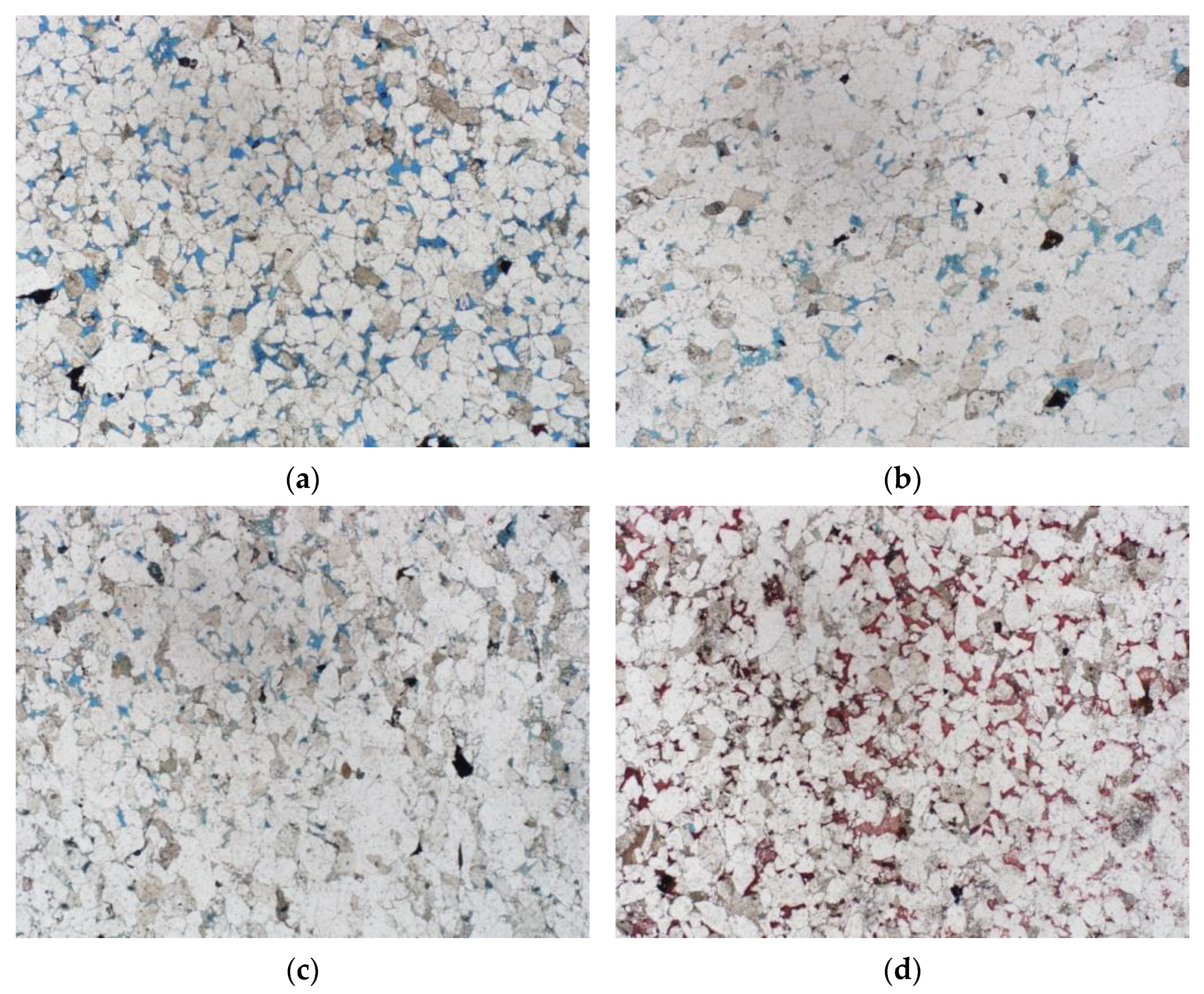
According to the thin-sections analysis, the pore types of the granite group in the No. 2 gas field are mainly secondary dissolved pores (Figure 1), followed by primary pores. The secondary dissolved pores mainly include intergranular enlarged dissolved pores, intergranular dissolved pores, and intragranular dissolved pores, among which intergranular dissolved pores (including certain primary pores) are relatively developed. Due to the difference of the sedimentary environment and complex diagenesis, the pore structure of the low-permeability and tight sandstone in this area is obviously different. The deeper the burial depth is, the stronger the compaction, and the worse the reservoir’s physical properties and microscopic pore structure.

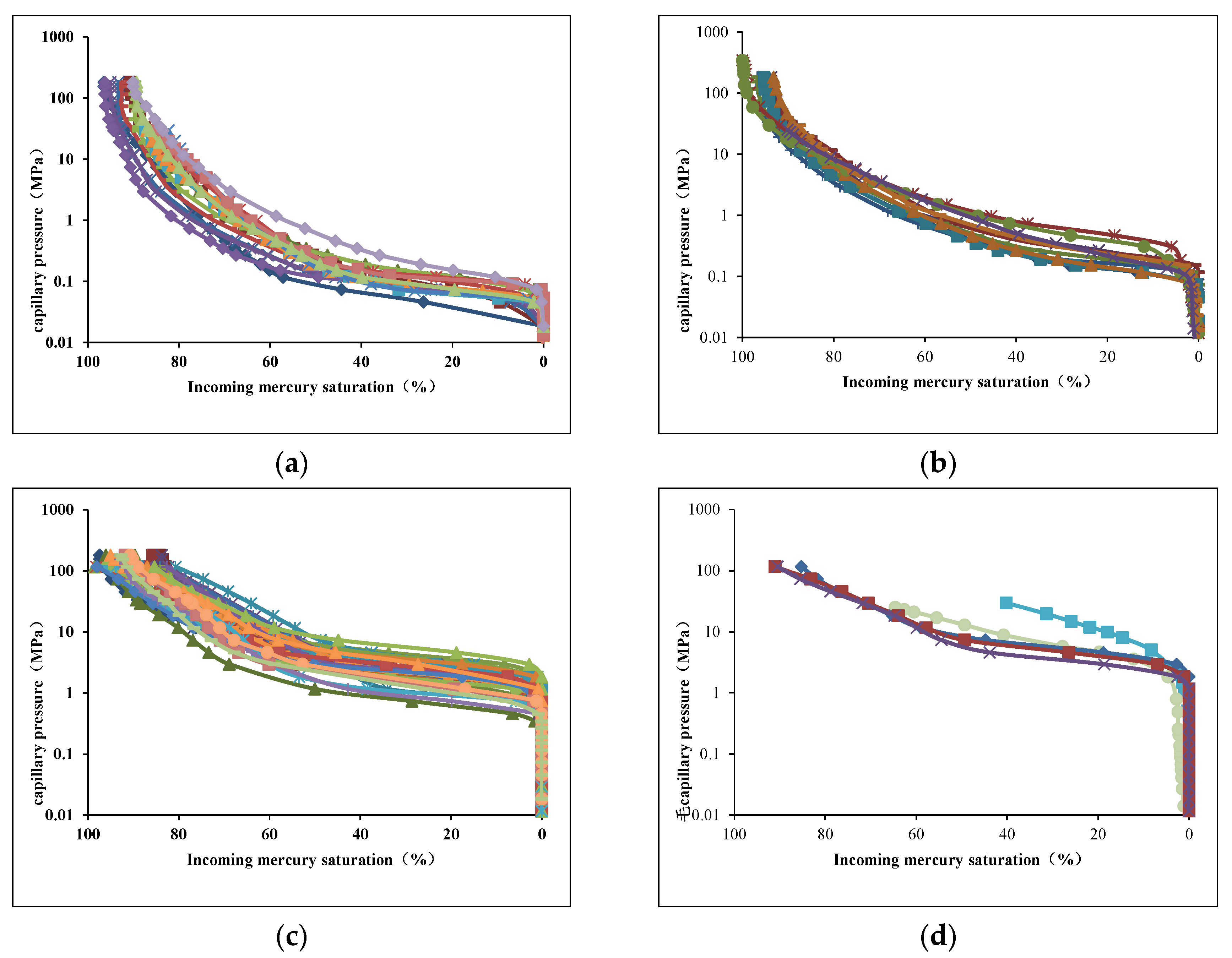
We have used more than 200 cores from the granite group of the No. 2 gas field in the X depression and have completed many core mercury injection experiments. According to the mercury quantity curve, displacement pressure, pore throat size, sorting, and other parameters of the mercury injection analysis, we can divide the mercury injection pore throat structure of the granitic formation reservoir in the X depression into four categories. According to Figure 2: the type I reservoirs (the Figure 2a) have a low displacement pressure and a long curve platform, indicating that this kind of sample has a thick pore throat, good sorting, and good physical properties. The displacement pressure of the type II reservoir (the Figure 2b) is higher than that of the type I reservoir, and the curve platform is shorter than that of the type I, indicating that the samples of the type II reservoir have a coarse pore throat, relatively good sorting, and moderate petrophysical properties. The drainage pressure of the type III reservoir (the Figure 2c) is higher than that of type II, with a shorter curve platform, worse sorting, and worse petrophysical properties. The drainage pressure of the type IV reservoir (the Figure 2d) is slightly higher than that of type III, with the worst sorting, the worst pore structure, and the worst petrophysical properties. Generally speaking, the mercury injection curve platform from the type I to type IV reservoirs gradually become shorter and steeper, and the displacement pressure gradually increases, reflecting the gradual deterioration of the petrophysical properties and pore structure of the type I~IV reservoirs.

According to the conventional petrophysical properties and mercury injection capillary data, we can count the characteristic parameters of the pore structures of different types of reservoirs. As shown in

Table 1. The characteristic parameters of pore structure of different types of reservoirs.

Characteristic Parameters		Type I	Type II	Type III	Type IV
Porosity	Min–Max average	6.3–11.7 9.0818	2.2–9.3 7.0341	4.2–10.7 7.4570	4.8–9.2 7.5242
Permeability		2.68–44.1 13.5927	0.0571–4.98 1.5145	0.0441–1.14 0.3719	0.0487–0.347 0.1995
FZI		8.4012–16.1130 11.1375	3.6318–7.7962 4.6052	2.2030–3.6103 2.7048	1.4562–2.1901 1.9653
Average pore throat radius		6.3411–11.6802 8.0570	0.0669–10.7238 2.9791	0.0822–9.3295 0.4873	0.0704–0.3263 0.2139
Drainage pressure		0.001–0.01 0.0092	0.01–2 0.3851	0.01–2 0.6737	0.5–3 1.1371
Skewness		0.9776–2.2866 1.5730	0.4871–2.2819 1.0584	0.4785–2.2393 1.8145	1.2890–2.1039 1.7332
Sorting coefficient		2.7051–3.5026 3.0179	1.8729–5.37778 2.8645	1.7733–4.4658 2.6378	1.8113–4.5918 2.7015
Mercury removal efficiency		14.4244–24.4350 20.6359	3.8785–49.0197 27.0564	12.9628–50.6256 32.1902	24.5102–67.0768 35.4130

, we can see that there are obvious differences between the different reservoirs with respect to the pore structure characteristic parameters, such as permeability, average pore throat radius, drainage pressure, skewness, sorting coefficient, and mercury-removal efficiency.

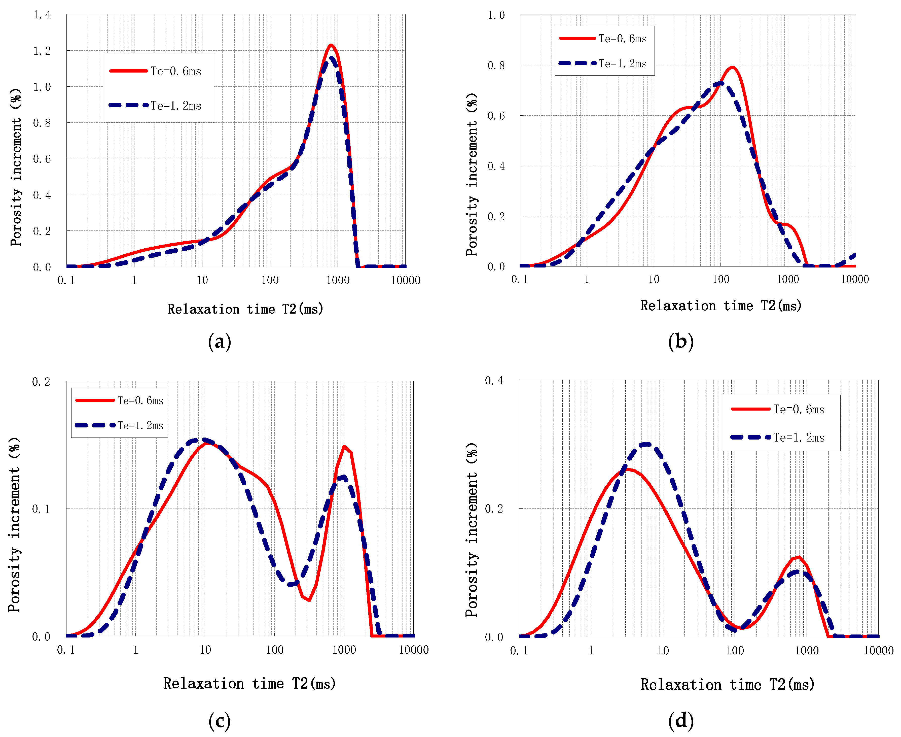
Figure 3 shows the typical nuclear magnetic T2 spectrum characteristics of the reservoir types with different pore structures in the study area. From these figures, we can see that the position of the main peak (the peak with the largest amplitude) of the T2 spectrum of the rock samples with a type I pore structure is between 100~1000 ms. The same value of the type II reservoir is close to 100 ms, for the type III reservoir it is close to 10 ms, and for the type IV reservoir it is less than 10 ms. This shows that the amount of clay bound water of the type IV reservoirs is the highest, followed by type III, and only a small portion of clay bound water is contained in type I and type II reservoirs. At the same time, the T2 spectrum shows that the component content of large pores in the type I reservoirs are the highest, while there is almost no large pore component in the type III and IV reservoirs, which reflects the complexity of the pore structure of a low-permeability tight sandstone reservoir, and the nuclear magnetic pore structure type is consistent with the mercury intrusion pore structure type.

3. Influencing Factors of Permeability in Tight Sandstone Reservoirs

3.1. Effect of Sedimentary Facies on Permeability

The sediment source condition is the main factor affecting the reservoirs, which controls the particles that make up the rock and the composition and content of cement and affects the thickness of the sand body. The distance between the sand body and the material source controls the particle size and sorting of the reservoir rock particles. If the material source supply is sufficient, the sandstone reservoir has a large thickness and wide extension range. Reservoirs belonging to different sedimentary facies have different particle structures, composition, structures, and other attributes, resulting in different permeability characteristics [13,14]. The X depression granitic formation is a sedimentary pattern involving a north river and a south lake as a whole. This means that the main part of the braided river is located in the north of the depression, and the braided river delta front is developed in the south-central area of the depression. According to the different lithology and typical combination characteristics, it can be subdivided into an underwater distributary channel, an estuary bar, sheet sand, a remote sand bar, and sedimentary microfacies between the underwater distributary channel. Macroscopically, underwater distributary channel sand bodies are far away from the source, but they are transported by hydrodynamic forces and their content of impurities is low, the dissolution has improved their pores, and their pore connectivity is good. This type of sand body belongs to the type I reservoir, which is defined by its remote provenance. The sand body of the remote sand bar is gradually weakened by hydrodynamic forces, and the lithology is mainly medium-fine sand, which corresponds to the characteristics of Type II. The sheet sand and remote sand bars are remote sand bodies with fine-silt sand as the main lithology, corresponding to the characteristics of Type III and Type IV reservoirs.

3.2. Influence of Pore Structure on Permeability

The pore structure of the reservoir mainly refers to the size, distribution, and connectivity of the pores and throats of the rock; the geometry of the pore and throat space; and the connectivity between the pores and throats. From the perspective of the relationship between the core porosity (φ) and permeability (K) of the granite group in the X depression (Figure 4), there is an overall trend of an increasing K with an increasing φ, but the porosity and permeability cannot be expressed by a single fitted relationship. When φ > 5% and the core porosity is similar, the permeability difference can reach two orders of magnitude. When K < 1 × 10⁻³ μm², it will be more concentrated. When K > 1 × 10⁻³ μm², the relationship is dispersed. This shows that permeability is not only affected by porosity, but also by other factors.

Since the permeability distribution is concentrated below 1 × 10⁻³ μm², we have established pore distribution histograms for when the rock samples comply with K < 1 × 10⁻³ μm², 1 × 10⁻³ μm² < K < 5 × 10⁻³ μm², and K > 5 × 10⁻³ μm² (the porosity of the sample is between 5% and 9%). As shown in Figure 5, when K < 1 × 10⁻³ μm², the pores with a small pore size account for a large proportion; with the increase in K, the pores with a large pore size component increase slightly. When 1 × 10⁻³ μm² < K< 5 × 10⁻³ μm², the large pore size component increases more obviously as K increases. When K > 5 × 10⁻³ μm², the large pore size distribution accounts for a large proportion. It can be seen that the permeability is greatly affected by the pore size distribution; that is, the pore structure is also one of the factors affecting the permeability, and the permeability of the reservoir is affected by the combination of porosity and the pore structure.

4. Flow Zone Index Method for Pore Structure Evaluation

4.1. Flow Zone Index FZI Method

The flow unit is the generic unit of the reservoir formed by various geological processes. It is a comprehensive product of the interaction of sedimentation, diagenesis, and, later, transformation. At present, the subdivision layers of the reservoirs in China basically remain on subdivided single sand bodies. In a narrow sense, the flow unit subdivides the single sand body, and further subdivides the reservoir based on the rock properties that affect the fluid flow and adopt a completely different standard from the subdivided single sand body [15]. The FZI method of the flow unit index is widely used. Obviously, the result of the flow unit method is more detailed, which is very important for subdividing sandstones with large differences in pore structure. Therefore, through the research and division of flow units, it is possible to reasonably divide and evaluate the reservoirs, and then predict the distribution of the reservoirs. The division of the reservoir flow units can be divided into two steps [16]. The first step is to determine the distribution of the connected sand bodies and seepage barriers, and the second step is to determine the seepage differences inside the connected bodies. Flow units with good fluidity can often be used as oil and gas reservoirs; flow units with poor fluidity often play a role in blocking the vertical and lateral flow of fluids and can still be used as poor oil and gas reservoirs. The flow units in which fluids cannot flow, mainly pure mudstone deposits and other tight rock formations, can be used as barriers for fluid flow.

In a homogeneous medium system, Kozeny proposed a permeability calculation formula via the capillary theory. Carman proved the reliability of the formula and established the Kozeny–Carman Equation [17,18]. Its common form is:

$$K=\frac{a}{S_{\mathrm{gv}}^2}\left[\frac{{\phi }_e{}^3}{{\left(1-{\phi }_e\right)}^2}\right],$$

(1)

In the formula: K is the permeability, 10⁻³ μm²; φ_e is the effective porosity; a is the regional empirical constant; S_gv is the surface area of the particle per unit volume.

Finally, Amaefule [19] formally proposed the flow unit index method (FZI) in 1983. Its principle is based on the average hydrodynamic unit radius theory. The Carman equation was modified to obtain the porosity–permeability relationship under different flow unit types:

$$K=\frac{1}{F_S{\tau }^2{S}_{\mathrm{gv}}^2}\left[\frac{{\phi }_e{}^3}{{\left(1-{\phi }_e\right)}^2}\right],$$

(2)

which transforms into:

$$\sqrt{\left(K/{\phi }_e\right)}=1/\left(\sqrt{F_s}\tau S_{\mathrm{gv}}\right)·{\phi }_e/\left(1-{\phi }_e\right),$$

(3)

In the formula: F_S is the shape factor; τ is the degree of curvature of the porous medium; S_gv is the surface area of the particle per unit volume; φ_e is the effective porosity; the unit of permeability is (×10⁻³ μm²).Then, it is necessary to define the following parameters:

Reservoir quality index:

$$RQI={10}^{-2}\cdot \pi \cdot \sqrt{\frac{K}{{\phi }_e}},$$

(4)

Standardized porosity index, which is the ratio of pore volume to the particle volume:

$${\phi }_Z=\frac{{\phi }_e}{1-{\phi }_e},$$

(5)

Then the flow stratification index:

$$FZI=\frac{1}{\sqrt{F_S}\tau S_{gv}}=\frac{RQI}{{\phi }_Z},$$

(6)

Take the logarithm of both sides of the above equation to obtain:

$$logRQI=log{\phi }_z+logFZI,$$

(7)

From the Formula (7), it can be seen that in the RQI and double logarithmic graphs, the two are shown as a double logarithmic linear relationship with a slope of one, and the intercept is FZI. For heterogeneous reservoirs, the relationship between RQI and φ_z is a cluster of parallel lines. Amaefule believes that samples with similar flow conditions fall approximately on the same straight line and belong to the same type of flow unit.

4.2. The Relationship between Flow Zone Index FZI and Pore Structure

The FZI is widely used by scholars at home and abroad as a quantitative identification and division of flow units, but the RQI/φ_z has no obvious geological significance. If K and φ_e are increased or decreased by a suitable multiple at the same time, the same FZI value will be obtained. Therefore, the division of flow zones according to the FZI may lead to the wrong conclusion wherein high-porosity and high-permeability reservoirs and low-porosity and low-permeability reservoirs are classified as the same type of flow unit, which does not meet the requirements of the smallest difference in storage properties within the flow unit and the largest difference in storage properties between different flow units [20]. Therefore, it is necessary to analyze the relationship between the flow zone index, FZI, and the pore structure to determine whether the flow zone index (FZI) can characterize the difference in permeability of the reservoirs inside different flow units.

The parameters that can better reflect the pore structure of the reservoir are mainly derived from the displacement pressure, the median saturation pressure, and the pore throat radius calculated based on the core mercury injection capillary pressure curve. However, using these parameters, it is difficult to establish a correlation with conventional logging, which is not convenient for practical application in the development stage. The flow zone index (FZI) is a parameter that combines the characteristics of rock minerals and the pore throat structure to determine the pore structure, which is theoretically similar to the capillary pressure curve.

From the mercury injection capillary pressure curve, we extract the parameters of the maximum pore throat radius R_max, displacement pressure P_d, and average throat radius R, and analyze the correlation between these three pore structure characterization parameters and the flow zone index (FZI). Through the analysis, we find that the FZI increases with the increase in the maximum pore throat radius R_max and the average throat radius R, and decreases with the increase in the displacement pressure Pd, and they are well correlated (as shown in Figure 6). It can be seen that in the granite group of the Ningbo gas field in the X depression, the flow zone index (FZI) can effectively reflect the pore structure characteristics of a low-permeability dense sandstone reservoir and can be used as a parameter to characterize the permeability difference between different flow units. Therefore, we use this parameter as the basis for the classification of flow units and the evaluation of the corresponding reservoir pore structure.

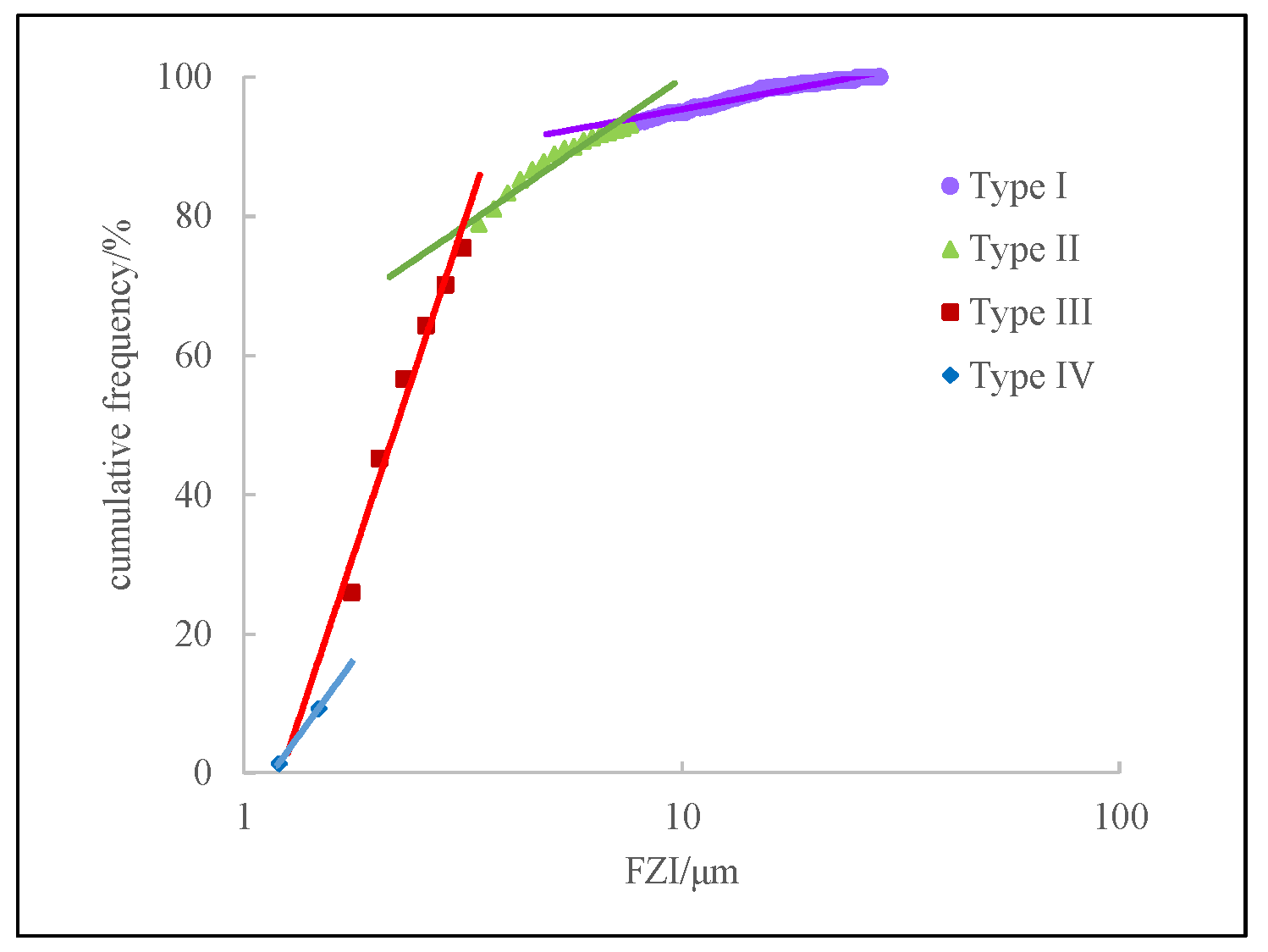
4.3. Division of Different Flow Units by Cumulative Frequency of Flow Zone Index (FZI)

The reservoirs in the same flow unit have similar petrophysical, pore structure, and fluid seepage characteristics. Therefore, the flow zone index (FZI) of the reservoirs with similar characteristics shows a straight line on the cumulative frequency curve, and the number of straight lines with different slopes corresponds to the number of flow unit types. Based on the analysis data of more than 1100 cores in the granite group of the No. 2 gas field in the X depression, we draw the relationship between the formation’s FZI and the cumulative frequency.

As shown in Figure 7, the cumulative frequency curve of the formation’s FZI of the granite group has obvious segmentation and can be divided into four trend lines with different slopes. Thus, we can classify the core of the sample points into four types of flow units, and the specific classification criteria are shown in

Table 2. Classification criteria for different flow units in low-permeability tight reservoirs of granitic formation in No. 2 Gas Field.

Flow Unit Type	FZI/μm	Porosity/%	Permeability/10−3 μm2	Number of Samples	Sample Proportion/%
Type I	>7.76	0.629–8.082	0.011–6.139	80	6.8
Type II	3.15~7.76	1.2–8.9	0.008~1.578	237	20.1
Type III	1.47~3.15	2.22–10.1	0.009~0.836	810	68.8
Type IV	<1.47	4.65–8.0	0.022~0.113	50	4.3

.

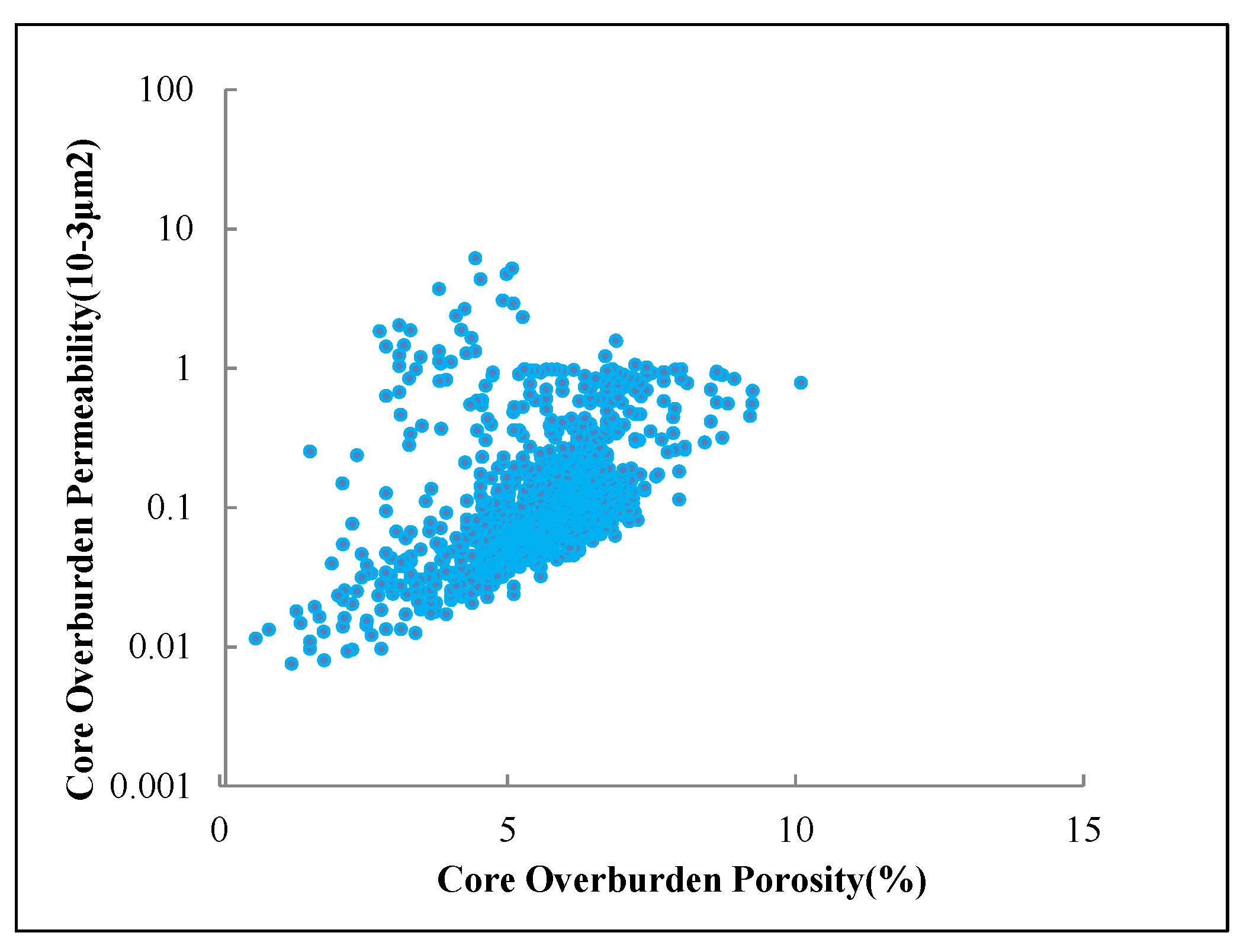
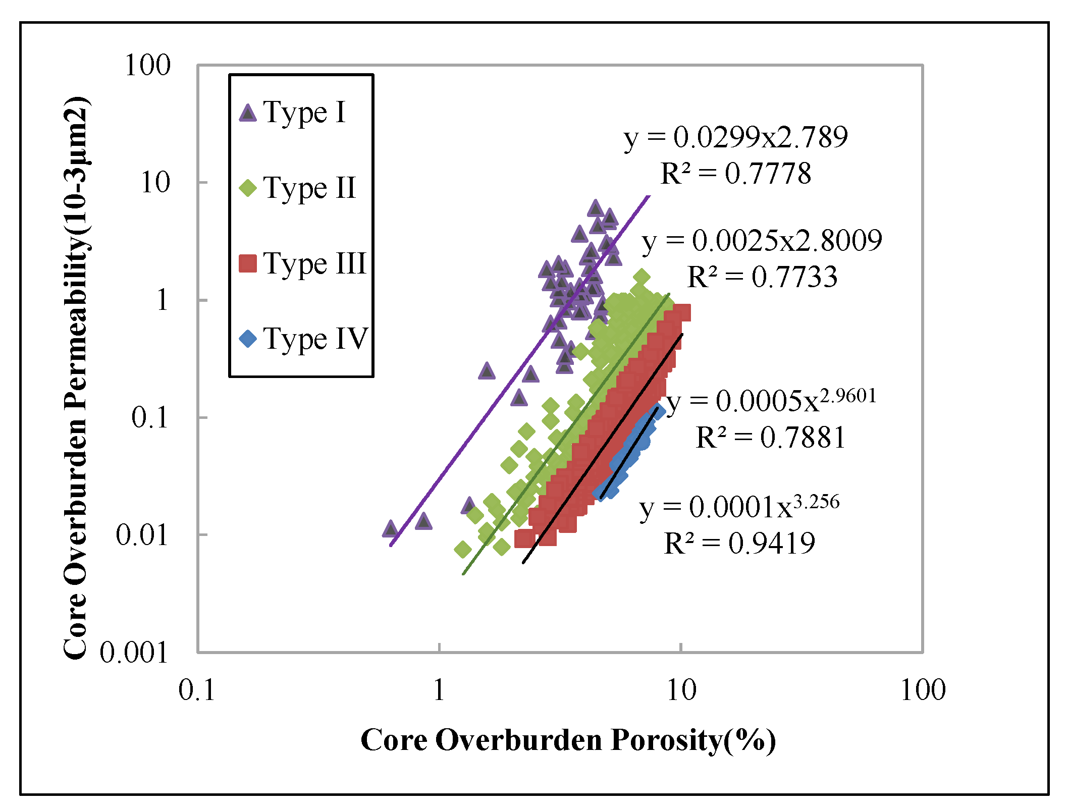
According to the data in Table 2, the main flow unit type in the low-permeability tight reservoir of the granite group is type III with poor physical properties, accounting for 63.3%. The type I flow unit with the best physical properties accounts for only 6.8%. The characteristics of the low-permeability tight sandstone reservoirs in the study area are further verified. At the same time, according to the FZI classification standard, the physical property boundary between each type of reservoir tends to be clear. After classification, the correlation between the porosity and permeability of the low-permeability tight reservoir in the granite group is significantly improved (Figure 8), which further shows that the formation’s FZI can effectively reflect the pore structure characteristics of the granite group reservoir and accurately classify reservoirs with different pore structures.

According to the classification of different flow units, we established the corresponding permeability calculation model:

$$\begin{gathered} K_{\mathrm{I}}=0.0299{\phi }^{2.789} \\ {K}_{\mathrm{II}}=0.0025{\phi }^{2.8009} \\ {K}_{\mathrm{III}}=0.0005{\phi }^{2.9601} \\ {K}_{\mathrm{IV}}=0.0001{\phi }^{3.256} \end{gathered}$$

(8)

In the formula, the subscripts I, II, III, and IV represent the reservoirs of type I, II, III, and IV, respectively.

4.4. Relationship between FZI of Core Section and Logging Curve of Corresponding Depth Section

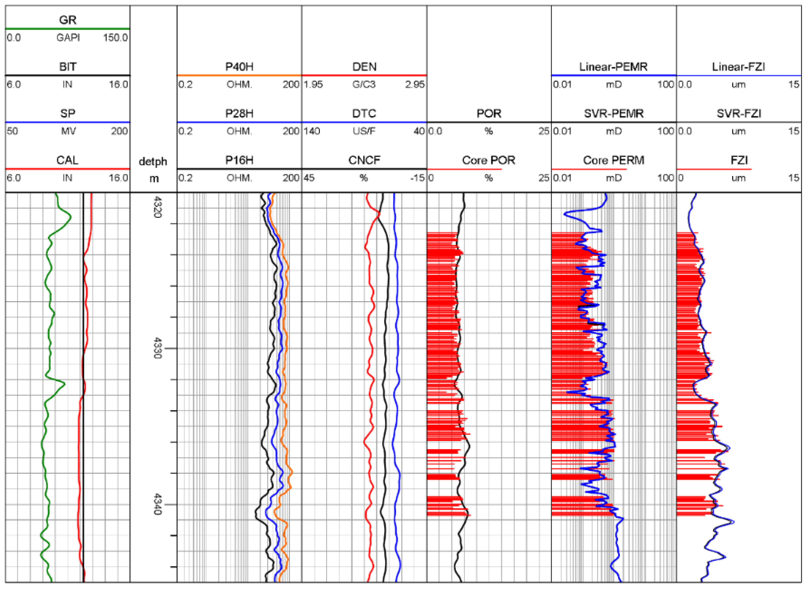
In the process of actual logging data processing and the interpretation of a single well, it is necessary to establish the relationship between the FZI of the core section and the logging curve of the corresponding depth section and apply the established relationship to the non-coring section to obtain an accurate continuous permeability curve. To establish the relationship between the flow unit index FZI of the core section and the logging curve, the first step is to select the logging data with an obvious response to FZI.

Figure 9 is the conventional logging response diagram of the 4320–4345 m well section of Well X1 in the No. 2 gas field. According to the test data, the 4322–4345 m section of Well X1 is a gas layer. In the 4222–4341 m coring interval, when the natural gamma value increases, the permeability and FZI have the characteristics of an obvious decrease. The resistivity of the coring section is relatively high. As the depth further deepens, the magnitude difference between the deep resistivity and the shallow resistivity increases, and the physical properties of the reservoir are obviously improved. The porosity, permeability, and FZI have a significant positive correlation. At the same time, it is found that there is a correlation between the acoustic transit time and porosity. Compared with the neutron curve, the acoustic transit time is not sensitive to the fluid properties and can also reflect the pore type and pore structure characteristics to a certain extent.

4.4.1. Support Vector Regression

The methods of establishing the relationship between the FZI and logging curve include the multiple linear regression method [21,22,23] and the support vector regression (SVR) method [24,25]. As the most commonly used regression method, the multiple linear regression is based on the least squares method [26] and empirical risk minimization is its criterion, while support vector regression is based on a linear kernel function and structural risk minimization as the criterion. With the addition of slack variables, the support vector is more robust to outliers than the multiple linear regression method.

This paper will use the Support Vector Regression (SVR) method and validate it with a multiple linear regression. Support vector regression is the realization of the support vector machine to solve the regression problem, and it is the approximate realization of the structural risk minimization method in the neural network system. The basic idea is to transform the input into a high-dimensional feature space and find an optimal classification plane in the high-dimensional space to maximize the classification interval. In the nonlinear case, the classification hyperplane is:

$$f\left(x\right)=wh\left(x\right)+b, w\in R^m,b\in R,$$

(9)

where w and b represent the normal vector and intercept of the hyperplane, respectively, and h (x) represents the nonlinear mapping function. The objective function is expressed as:

$$\min 0.5\times {\left|\left|w\right|\right|}_2{}^2+C\epsilon ,$$

(10)

Restrictions:

$$y_i\left(w^T{x}_i+b\right)\ge 1-{\epsilon }_i\left( i=1,2,\dots ,\mathrm{k}\right) ,$$

(11)

where $x_i$ is a cluster of points, $y_i$ is the corresponding category, k is the number of samples, ${\epsilon }_{i }$≥ 0 is the slack variable, and C is the penalty factor

When the support vector machine is dealing with regression, it tries to fit more data to the interval; the width of the interval is controlled by the hyperparameter epsilon, while the data are indifferent to the loss in the interval band, and finally, by minimizing the total loss and maximizing the interval, one can obtain the optimal model and achieve better generalization.

Support vector regression also provides a kernel function, which can be used to fit both linear and nonlinear functions effectively. Commonly used kernel functions include linear kernel, polynomial kernel, Gaussian kernel, Laplace kernel, and Sigmoid kernel.

According to the data characteristics of the FZI, this study performs logarithmic processing on the FZI value, uses linear kernel function fitting, determines the optimal curve participating in the regression through a correlation analysis, and uses the grid optimization algorithm to find the optimal model parameters. The vector machine regression operation process reduces the complexity of the fitting function and improves the accuracy and applicability of the fitting results.

4.4.2. Calculation of FZI by Multiparameter Fitting

Through the analysis of the conventional logging response data, it can be seen that the natural gamma, density, acoustic wave, and resistivity curves have obvious response characteristics, and the correlation between the five normalized curves and the FZI is obtained by using the correlation algorithm (

Table 3. Correlation analysis between single curve and ln (FZI).

Curve Name	DTC	GR	DEN	P16H	P40H
Correlation with ln (FZI) (decimal)	0.3	−0.67	−0.068	−0.7	−0.042

).

Considering that the gamma rays will be absorbed by the formation, its absorptive capacity is related to the formation density, and the ratio of induced resistivity can reflect the permeability of the reservoir. After a comprehensive consideration, the combination of the ratio of the gamma to the density and the ratio of the acoustic wave to the induced resistivity are used to fit the FZI. The correlation between this combination and the ln FZI is shown in

Table 4. Correlation analysis between combination curve and ln (FZI).

Combined Curve Name	GR/DEN	DTC	P40H/P16H
Correlation with ln (FZI) (decimal)	−0.69	0.3	0.85

. After the combination, the correlation of the resistivity is increased by about 20%, and the correlation of the natural gamma is increased by 3%. The effect of the combination curve can be demonstrated more clearly.

Using the same combination curve to perform least squares fitting, the FZI response equation is obtained as:

$$\ln FZI =-0.003\times \mathrm{DTC}-0.047\times \left(\frac{\mathrm{GR}}{\mathrm{DEN}}\right)+0.427\times \left(\frac{\mathrm{P}40\mathrm{H}}{\mathrm{P}16\mathrm{H}}\right)+1.41, R^2=0.77,$$

(12)

Under the support vector machine parameters C = 1, ε = 0.09, the response equation of FZI is obtained as:

$$\ln FZI=-0.006\times \mathrm{DTC}-0.048\times \left(\frac{\mathrm{GR}}{\mathrm{DEN}}\right)+0.418\times \left(\frac{\mathrm{P}40\mathrm{H}}{\mathrm{P}16\mathrm{H}}\right)+1.67, R^2=0.77,$$

(13)

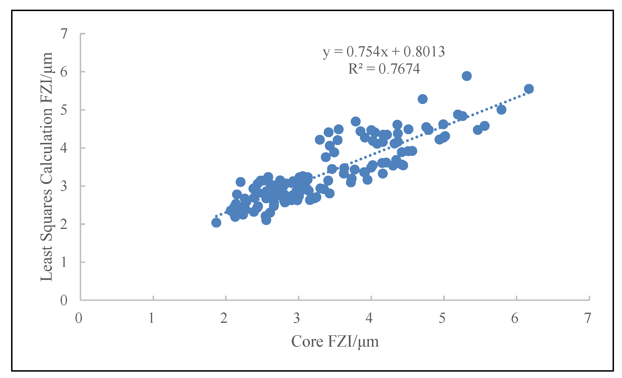
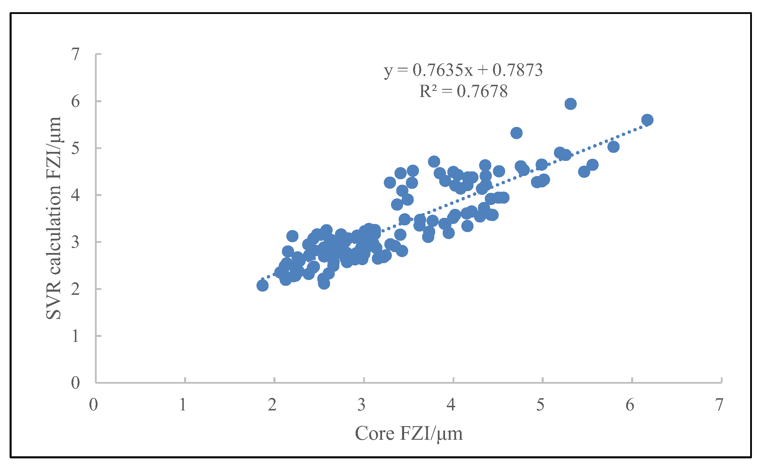
Then, use this model for back judgment. Figure 10 and Figure 11 are the comparison charts of the FZI values calculated by the linear regression method and the support vector regression method, respectively, and the fitting effects of the two methods verify each other, which verifies the reliability of the fitting.

5. Case Analysis

The gas interval is 4320–4345 m in Well X1, with a total of 145 cores. The porosity distribution of this gas interval is 3%~9%, and the average porosity is 6.25%; the permeability distribution is 0.004~1.025 × 10⁻³ μm², and the average permeability is 0.387 × 10⁻³ μm². The latter is mainly distributed in the second and third types of flow units. According to the established flow unit stratification standard and the relationship model between the logging curve and FZI, the continuous FZI curve of Well X1 in the study area was calculated, and the corresponding permeability was further calculated to obtain the logging interpretation result in Figure 9. The fifth track in the figure is the porosity curve calculated via the optimization algorithm. Compared with the core overburden porosity, the absolute error is 0.47%, and the relative error is 6.54%. The sixth track is the permeability curve calculated by the support vector machine regression and the least squares method after the reservoir classification based on the FZI. Compared with the core overburden permeability, the absolute errors of the calculated permeability are 0.45 × 10⁻⁴ μm² and 0.48 × 10⁻⁴ μm², while the relative errors are 10.67% and 11.35%, respectively. Track 7 is the calculated FZI value. The calculated permeability after classification has high accuracy, and the calculated permeability is in good agreement with the core overburden permeability, which meets the requirements of a fine reservoir evaluation.

6. Conclusions and Discussion

(1)

Through an analysis of the characteristics of the porosity and pore structure in the study area, it was found that porosity and pore structure are the two key factors affecting the permeability. Further analysis found that the three pore structure characterization parameters had a good correlation with the flow unit index FZI, and the FZI can effectively reflect the pore structure characteristics of low-permeability-tight sandstone reservoirs in the study area. Based on this, the accuracy of the permeability model established after the reservoir classification is significantly improved.

(2)

On the basis of the response characteristics of the conventional logging data, the correlation analysis between each curve and the FZI was established through machine learning, and the optimal curve combination was selected to establish a multi-parameter fitting equation of the flow unit index, which can realize the continuous evaluation of permeability and lay the foundation for the fine evaluation of the permeability of low-permeability tight reservoirs.

(3)

There are two errors in the calculation of the FZI and the calculation of permeability in the current classification. The accumulation of errors will affect the calculation accuracy. We can try to combine other classification algorithms to avoid the calculation of the FZI and directly divide the flow unit types to reduce error transmission.