Abstract
An excess non-linear and unbalanced load application increases the power quality (PQ) problem by injecting harmonic current. The avoidance of neutral current control creates additional PQ problems due to excess circulating current in modern 34W applications. Therefore, this manuscript suggests improved transform-based voltage and current control approaches for both 33W and 34W shunt active filter (SAF) applications. In the proposed approach, a novel combined voltage and current (NCVC) control approach is presented for modern 33W systems by using voltage and closed-loop current controllers. However, due to the absence of a neutral current, the NCVC is not sufficient for 34W system application. Therefore, by considering the current reference parameter generated from the NCVC, a novel harmonic compensation technique (NHCT) is proposed with proper mathematical expressions for the 34W application. To show the importance of NHCT over traditional P-Q-R control, the developed MATLAB/Simulink model is tested by using different 1 and 3 nonlinear/unbalanced load conditions. The comparative results indicate that, by using NHCT, the 34W system contains a lesser total harmonic distortion (THD) and harmonic mitigation ratio (HMR), less ripple frequency, an improved power factor, a lesser neutral current, and a balanced active/reactive power condition. From the above comparative analysis results, it is found that the overall improvement percentage is 66.78%. The above findings justify the significance of the NCVC and NHCT approach during both unbalanced and non-linear load-based 34W applications.
1. Introduction
1.1. Harmonic Problem Associated with Modern Load Applications
The distribution sector faces many challenges due to the varying loads, non-linear/unbalanced loads, reactive power demand, and harmonic current issues [1]. Power system voltage is distorted due to the absorption of nonlinear current harmonic components [2]. The presence of both non-linear voltage and current in a power system increases the instability, frequency imbalance, and power losses in the line; reduces the power factor; and affects the performance of the sensitive load [3]. Generally, the nonlinear currents and voltages by 3 non-linear loads like motor drives, thyristor-based rectifiers, and uninterruptible power sources (UPS) have both positive (7th and 13th, etc.) and negative (5th and 11th, etc.) sequence harmonics [4]. However, the non-linear current and voltage produced by using 1 non-linear load like a switch mode power supply (SMPS) [4] are attached to a 1 to neutral current in a 34W power system to produce the three-order zero-sequence harmonics (3rd, 9th, 15th, etc.) [5]. As a result, the above-generated positive and negative sequence components and the three-order zero-sequence harmonic currents are added arithmetically at the neutral bus [6]. Therefore, in 34W power system application, the magnitude of the neutral current is increased to 1.75 times that of the phase current [7] and affects the power quality (PQ). In addition to that, defective cables and overheating transformers generate an additional, third harmonic component, and these components also affect the system’s efficiency and stability. Hence, in modern power applications, there is a need to regulate the neutral current and harmonics within the specified limit.
1.2. Evolutions of Filters and Associated Problems
For a stable and improved performance at the generation [8], distribution [9], and transmission [10] sectors, the above nonlinearity and PQ issues must necessarily be addressed. As a solution, conventionally, electromechanical devices such as tap changing transformers [11], passive filters [12], and synchronous condensers [13] are used to solve the PQ-related problems. Generally, passive filters are widely chosen due to their simple design and lower cost. However, conventional passive filters cannot eliminate the harmonic/non-linearity due to an increase in size, fixed reactive power supply and improper tuning of the resonance, etc. [13]. As a solution, power electronic-based devices like the dynamic voltage restorer (DVR) [14], shunt and series active filter [15], static compensator [16], and unified power quality controller (UPQC) [17] are widely selected to resolve the PQ related problems. Still, due to the requirement of excess power electronic switches and fixed compensation, shunt active filter (SAF)-based voltage source inverters (VSIs) are selected for simple design, economy, and better performance [18]. In addition to that, SAFs are used to eliminate the harmonics/non-linearity through a variable frequency and reactive power supply [19]. However, this type of filter integration is only feasible for 33W system applications, and the performance is affected due to the excess circulating current present in the system [20,21]. In a practical system, the role of a neutral current path is very important: to protect the system from sudden surges or transient conditions [22]. In [23,24], a four-leg SAF-based VSI is chosen for 34W system applications and facilitates a neutral current path to eliminate the circulating current. However, to get optimal performance in terms of reduced switching loss and proper switching signal generation, finding a better and more robust control technique for four-leg SAFs is necessary [25]. Therefore, to overcome the above shortcomings, there is a requirement to find novel control strategies for reducing the switching losses, circulating current, and harmonics obtained from the non-linear load.
1.3. Need for Coordinated Control
In this section, the need for a novel coordinated controller is discussed by evaluating the merits and demerits of existing literature. In [26], for 3 SAF operations, a linear feed-forward control approach is recommended. However, the design of the above controller is complex with a linear control strategy for both steady-state and transient-state conditions because the active power filter contains multiple control inputs and state variables. Therefore, the traditional control approaches such as a linear quadratic regulator (LQR) [27] or linear Gaussian servo controller (LGSC) [28] are suggested for computing the switching pulses for the inverter. However, the above controllers do not provide significant performance during non-linear load applications and take more time to generate the pulses for inverter operation. In [29], due to the non-linear characteristics of the active filter, a sliding mode control (SMC)-based robust control strategy is suggested. However, in practical system application, the above strategies lag in their performance due to the chattering problems and the presence of additional noise [30]. The chattering problems are undesirable phenomena of oscillation that occur at constant frequency and amplitude [31]. Due to the above issues, the system lags in its performance by reducing the control accuracy, affecting the moving mechanical parts, and producing high heat losses in an electric circuit [32]. In [9,33,34], advanced control strategies are proposed for 34W operation. However, the robustness of the controller is identified only during balanced load conditions, and, during unbalanced load conditions, the PCC voltage is severely affected. To avoid the above problem, in [35,36], suitable modifications are proposed by reducing the sensor requirement to balance the PCC voltage irrespective of unbalanced load conditions. However, during the controller design, the engineers do not consider the zero-sequence component because of the delta connection of the transformer in [35] and the delta connection of a non-linear load [36]. In [37], two independent controllers are suggested for grid-forming and grid-following modes of operation. In [38,39], the unbalanced load voltage is compensated in the frame. Still, in [37,38,39], zero-sequence components are not considered during the controller design. For 3 applications, instantaneous power theory (IPT) is considered widely for simple design and implementation [40]. Therefore, the proposed concept is modified [41] and implemented for a 34W system operation [42]. In 33W [35] or 34W [43] system operation, IPT is used to compute the necessary compensating currents by assuming a linear utility voltage. However, during real-time applications, the utility voltage may be unbalanced or distorted. Under such circumstances, the control of the 34-leg SAF using the traditional IPT scheme does not offer better performance during non-linear and unstable load applications [44]. Therefore, designing an appropriate, effective controller for regulating the neutral and harmonic current at the desired limit during distorted utility voltage and non-linear/ unbalanced load applications is necessary.
1.4. Major Contribution towards Advancement
The primary objectives of the manuscript are presented as follows.
- Design of a new coordinated voltage and current control approach for 33W and 34W systems with lesser complexity and easier implementation.
- Development of a novel harmonic compensation technique (NHCT) by considering the reference current generated from an NCVC and verifying the controller through an original mathematical expression for the 34W microgrid system.
- Analysis of the impact of the neutral current and comparison of the proposed performance with the traditional P-Q-R approach.
2. Integration Problems and System Modeling
This section is divided into three subsections. In Section 1, the modern 33W and 34W Utility Grid with a distribution-flexible AC transmission system (DFACTS) and associated problems are discussed. Looking at the problems, the proposed system model organization with a detailed schematic diagram is presented in Section 2. To give a proper mathematical justification, detailed mathematical modeling of the proposed system for component extraction is presented in Section 3.
2.1. Modern 33W and 34W Utility Grid with DFACTS
In this section, the problems associated with the modern 33W and 34W utility grid with DFACTS are presented.
- The modern 33W utility grid requires three-leg insulated gate bipolar transistor (IGBT) switch-based DFACTS devices for compensating the harmonics and unbalanced loads. Among different types of DFACTS devices, preferably active power filters (APFs) are selected for balancing the voltage, frequency, and phase angle. APFs are used for specific applications like shunt and series compensation. The modern 33W utility system facilitates only three-phase non-linear and balanced/unbalanced load applications. The main problem associated with a 33W system is the lack of a return path for an unbalanced current, which leads to distortion of the grid voltage.
- The modern 34W utility grid requires four-leg IGBT-based DFACTS devices for alleviating neutral, harmonic, and unbalanced current components. APFs are also applicable for both shunt and series operations. This type of system is applicable for both single-phase and three-phase nonlinear and balanced/unbalanced load applications. This is more applicable to modern power system applications. In case of an unbalanced load, a neutral line provides a path for neutral current regulation, which reduces the circulating current issues. The main problem associated with the modern power system includes excess neutral current, non-linearity, and voltage regulation. For regulating the 34W system, an additional PWM is required, which is generated by the associated control method using the fourth wire of the system.
Looking at the above problems and modern power system needs, the regulation of both the 33W and 34W systems is a challenging issue. A proper controller design with an appropriate mathematical representation is much needed for real-time problems. The recommended features in the controller include robustness, speed, and adaptation to the system variations based on the current information related to single/three-phase nonlinear and unbalanced load applications. This motivates the development of a coordinated controller for both 33W and 34W utility-grid-based SAFs for modern power system applications.
2.2. System Organization
- The complete proposed system architecture is presented in Figure 1. In this proposed system architecture, a 34W grid is directly connected to the non-linear load. To see the variability, the non-linear load is converted to the unbalanced load through a C.B.
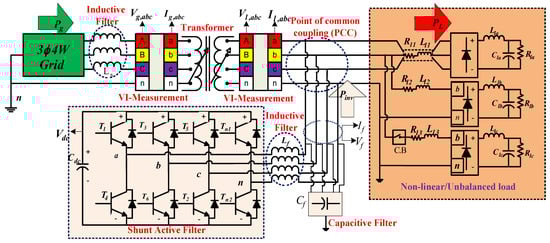 Figure 1. A 34W SAF_based coordinated power system schematic diagram.
 - As shown, a 34W-based voltage source inverter (34W-VSI) is designed by considering eight IGBT switches (T1, T2, T3, T4, T5, T6, Tn1, and Tn2) and a dc-link capacitor (Cdc). In this proposed system, the modeled 34W-VSI is connected to the system in quadrature.
- To eliminate the ripples present in the system, an additional LC filter is connected in series with the inverter.
- Disturbances like frequency variations, the dc-link voltage regulation, power factor, and harmonics are regulated through the proposed .
- Due to the shunt connection of the VSI and switches operated in the power frequency cycle, the inverter can behave as a shunt active filter and eliminates the nonlinearity present in the circuit. Thus, the system draws a balanced current from the grid and maintains a unity power factor.
2.3. Detailed Mathematical Modeling for SAF Component Extraction
The successful operation of SAFs depends on the required unbalanced load neutral current generation. Due to the above operation, the neutral grid current can be bounded to zero, and this shows the balanced operations of the grid. The complex power () and neutral current () equation of a non-linear-based system is represented as in [45,46].
Equation (1) shows that the complex power contains both balanced ( and ) and oscillating ( and ) components. In Equation (2), , , and are denoted as the phase currents presented in the 34W system. Due to the applications of non-linear and unbalanced load, the total power of the 34W system contains both harmonic and unbalanced components. Oscillating components are the combination of both harmonic and unbalanced components. The main purpose of using 34W SAFs is to eliminate the unbalanced/harmonic components and to achieve a unified power flow operation. During that period, the grid voltage and grid current must lie in the same phase (i.e., ,). To compute the required , the proper estimation of compensating current () plays an important role. Due to the shunt connection of the SAFs, also helps to eliminate the harmonic/unbalanced components present in the system. Therefore, there is a need for a proper mathematical representation for estimating the with the help of and , respectively. Then, the supplied Scomp can be computed as
where is termed as the supplied compensating current with a phase angle and computed as
where is termed as the supplied compensating voltage with a phase angle and is termed as the series impedance with a phase angle . The and components are computed by substituting Equation (4) in Equation (3) and presented as
From Equation (4), it is clear that the oscillating active/reactive power, and specifically the injected current, is regulated by controlling the SAF terminal voltage, current, and the associated impedance. Therefore, to achieve the above-planned objective, it is necessary to regulate the individual VSI switches so that the SAF impedance and nonlinear load impedance are converted to linear load and the system improves the PQ. Therefore, the switching operation of the SAF decides the control architecture of load compensation.
3. Coordinated Control Algorithm
In this section, the proposed coordinated control algorithm is designed by combining both NCVC and NHCT approaches for 33W and 3φ4W grid-connected non-linear and unbalanced load applications. The detailed controller performance with proper mathematical representations is discussed below. Initially, the detailed control algorithm of NCVC architecture for a 33W system is presented. By using the component extracted from NCVC, the proposed NHCT approach is structured for 34W system applications.
3.1. NCVC Architecture for a 33W System
To reduce the computational burden and reduce complexity, the proposed NCVC control architecture is presented for a 34W application by neglecting the zero-sequence component. In the proposed approach, the voltage controller regulates the real and reactive power. In addition to that, the current controller is used to regulate the inverter current output by selecting an appropriate switching sequence or modulation index. To obtain a complete idea, both the open-loop and closed-loop models with appropriate mathematical representation are discussed below.
3.1.1. Open-Loop PCC Voltage and VSI Controller
During the switched-on conditions of VSI, the open-loop VSI current control model is designed by using Kirchhoff’s voltage law (KVL) and represented in the component. The following equations are represented in the frequency domain. Frequency domain analyses are used to convert differential equations into simple algebraic equations [47,48].
The open-loop proposed VSI voltage control model is designed by using Kirchhoff’s current law (KCL) and represented in the component.
where Lf and Lg are termed as a filter and grid inductor, Rf and Rg are termed as the filter and grid resistance, Ron is termed as the switching on resistance, Cf is termed as a capacitive filter, and and are termed as the active and reactive current components. is termed as the combination of the active filter and grid current component, and is termed as the combination of the reactive filter and grid current components. , , and are termed as the active components of filter voltage, grid voltage, and load voltage, respectively. Similarly, , , and are termed as the reactive components of filter voltage, grid voltage, and load voltage, respectively. and are termed as the operating frequency and change in frequency due to the system variations.
3.1.2. Closed-Loop PCC Voltage Controller and VSI Controller
- ✓
- Working of the VSI Voltage Controller:
As stated in Figure 2, the main motive of the PCC voltage controller is to control the active and reactive components of the PCC voltage as per the desired grid voltage signals. To develop the voltage controller, specific filters such as a Notch filter (Fn(s)), capacitive filter, and regulators are required. The detailed description regarding filter selection as well as design is presented in Appendix A. Figure 2 shows that, at first, the three-phase grid voltage () and load current () components are converted to the two-phase grid voltage () and load current () components. The NCVC technique is only used to generate the signals by reducing the complexity and computational burden. To eliminate the higher-order harmonics from the voltage ( and ), a notch filter is used initially. After eliminating the harmonics, the sensed voltage signals ( and ) are compared with the reference voltage signals ( and ) to find the active and reactive error signals ( and ). The obtained error signal is linearized through the PI regulator. The selection of regulators is explained below. The reference voltage signal is also used to determine the frequency component through the capacitive filter and closed-loop frequency regulator. The detailed structure of the closed-loop frequency regulator is illustrated in Figure 3. The controller structure is designed by considering Equations (8) and (9). In addition to that, to eliminate the non-linearity present in the active () and reactive load (), the notch filter is used. After getting all the linearized values ( and ), the voltage controller extracts the linear active and reactive ( and ) current components. The sensed values are further used to design the current controller for VSI operation. The proposed PCC voltage controller references are determined by analyzing the active/reactive power, frequency, and power factor demand as illustrated in Figure 3. The undertaken controller design parameters are presented in Appendix B (Table A1).
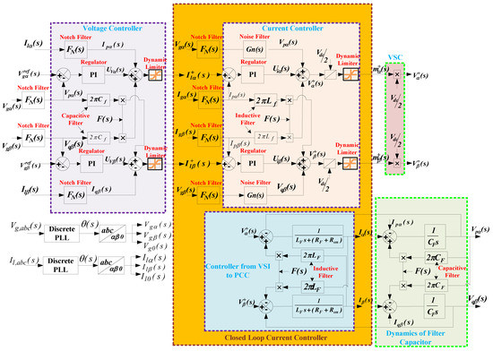
Figure 2.
NCVC architecture for 33W VSI application.
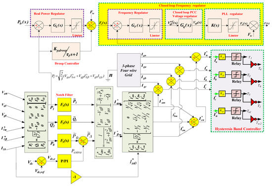
Figure 3.
Proposed NHCT control architecture.
- ✓
- Regulator Selection:
As one of the open-loop poles is already at the origin, the system achieves zero steady-state error conditions easily. Therefore, for harmonic elimination or avoidance of any uncertainty condition, the applications of the proportional controller have gained interest [19,26]. A higher value of the proportional gain is selected for faster system response, and a lower value is chosen to improve the system’s stability during any transient conditions. In these circumstances, the proportional integral regulators (PIR) are also preferred at one condition by avoiding the chances of pure integrator conditions; otherwise, the system loses its stability. To guarantee zero steady-state error, all the regulators used in the NCVC are generally PIRs. The zero of the PIRs is selected so that it cancels out the close to origin pole of the open-loop system. The selection of the PIR gain ‘K’ occurs in such a way that, for a more significant value, it gives a faster response. In addition, it limits the peak overshoot to a safer limit (if the root locus is drawn, for a stable reply, all the closed-loop poles are present on the left side of the s-plane at all PIR gain values). All the regulators of the current controllers are presented as
- ✓
- Frequency regulator:
As illustrated in Figure 3, the frequency of the proposed system is varied between 49.9 Hz and 50.1 Hz. The damping ratio () of both the frequency regulator and notch filter is set in between 0.5 and 0.8 to avoid a sluggish response. In this proposed approach, a first-order filter is used to limit the frequency variation. The details regarding the frequency regulator are detailed in Table A1. The regulator dynamics are tested and presented in the result analysis section.
- ✓
- Working of the VSI Current Controller:
The main motive of the VSI current controller is to control the inverter current by adequately regulating the grid current ( and ) by properly sensing and from the voltage controller. In the proposed voltage controller, after developing the necessary harmonic free components ( and ), and are passed to the current controller for appropriate inverter pulse generation by regulating the modulation index. The related parameters of the designed system were determined using an open-loop VSI current control model as presented in Equations (6) and (7). In this condition, a PI regulator is also used to linearize the error. Similar to the voltage controller, to linearize the grid currents ( and ), the actual grid currents ( and ) are passed through the notch filter. To reduce the high-order harmonics and facilitate faster operation, the grid’s active and reactive voltages are passed through both noise and notch filters. Noise filters are used to limit the undesired harmonics. The details are illustrated in Appendix A and B. The linearized voltages and are obtained from the filter components. Detailed explanations related to filter design are given in Appendix A. The obtained and are further compared with the noise-free components ( and ) obtained from the voltage controller to generate the error current signal. The error signal is passed through the PI regulator to linearize the current signals and . By combining all the linearized signals, the modulation indexes ( and ) are generated. By using this controlling method, the modulation index of the converter controller can be controlled. The desired current signals can be generated by controlling the modulation index as illustrated in Figure 2. An additional filter is also used to obtain the linearized voltage from the controller. This voltage signal can be used to generate the switching pulses for the inverter controller.
The overall NCVC controller is illustrated in Figure 2 for operation. Any one of the above controllers can be used to generate the switching pulses for the inverter. However, the proposed NCVC approach is not applicable for 34W-SAF systems due to the ignorance of the zero-sequence component. In 34W-SAF applications, the proper regulation of neutral current (In) plays an important role. Due to the dynamic ability of the controller, the voltage controller output current ( and ) generated from the NCVC controller is used to design the NHCT control architecture for 34W-SAF applications. The detailed mathematical operation with proper design is presented in the next section.
3.2. NHCT Control Architecture for a 34W System
Due to the excess non-linear/unbalanced load and 34W-SAF applications, the proposed NCVC controller is restructured and named a novel harmonic cancellation technique (NHCT). The proposed NHCT control architecture is illustrated in Figure 3. The main aim of designing the proposed NHCT controller is to reduce the circulating current present in the system and improve the PQ significantly. The obtained and from the NCVC approach are considered in designing the proposed NHCT architecture. Therefore, by using the voltage (, , and ) and current (, , and ) components, the instantaneous active power (Pl), reactive power (Ql), and extra power (P0) are computed and represented as
The active and reactive power components contain both average ( and ) and oscillating components ( and ) as stated in Equations (12) and (13). Both of the equations also show that and contain both harmonic (Ph and Qh) and negative sequence (Pn and Qn) components [12,13].
The total instantaneous oscillating active power () is computed by adding active power (), zero-sequence power (), and extra power extracted () from dc-link voltage, which can be represented as
For non-linear currents, reactive power mitigation, and linearizing the unbalanced load current, it is essential to eliminate all the associated oscillating reactive and current active components. Therefore, by considering all of the above factors, the mitigating current components ( and ) are computed as
In addition to that, the zero-sequence current (Il0) is also essential to compensate for reducing the circulating current and its effects. Therefore, the reference mitigating zero-sequence current () is computed as
The additional active power component () is computed as the sum of VSI extra power (Pextra) and Pextra. is used to balance the energy loss that occurs in the system and presents as
Pextra is an active power component obtained from the voltage compensator. The dc-link voltage compensator is modeled to provide both better harmonic mitigation and outstanding transient response. The operating dc-link capacitor voltage (Vdc) is compared with the reference dc-link voltage (Vdc, ref), and the error between the two components (Vdc,e) is passed through a P/PI regulator to obtain the Pextra component. In the proposed approach, to offer a stable and harmonic-free response, a suitable selection of the proportional and integral parameters (Kp and Ki) is highly essential. Moreover, this voltage compensator is highly needed during renewable energy integration to fulfill the grid power demand. The output of the PI regulator in time domain analysis is presented as
where is denoted as the active power component of the grid. As illustrated in Figure 4, the obtained transfer function of the PI regulator ‘’ is presented as
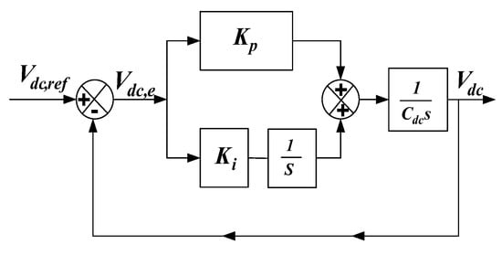
Figure 4.
Regulation of DC-link Voltage.
The overall open-loop and closed-loop transfer function of the dc-link voltage compensator ( and ) are computed as
Equation (21) indicates that is a second-order transfer function. From the above closed-loop transfer function, the damping ratio () and bandwidth () are computed as follows.
To ensure a linear relationship between the dynamic and static responses, the range of ‘’ is chosen between 0.5 and 0.8. The Bode response of at different is shown in Figure 5a. For different values, the phase margin of the system varies in between and . As shown in Figure 5a, at 284 rad/s bandwidth and phase margin, the system achieves a stable and linear response condition. By putting the , , and phase margin values in Equations (22) and (23), the Kp and Ki values are computed as 0.8 and 180, respectively. By using the computed Kp and Ki values, the Bode response of is demonstrated in Figure 5b. Figure 5b clearly shows that, by using the Kp and Ki values, the system responses become stable, and this also provide a faster response.
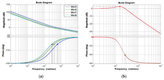
Figure 5.
Bode diagram of (a) at different bandwidths and (b) at the obtained Kp and Ki values.
After computing the compensating current components (, , and ), it is necessary to transform the current component to the ABC current component for generating the pulses for the inverter. The conversion (, , and ) is presented as
After computing the mitigating current component in the abc frame, the generated current components , , , and are compared with the grid current components (, ,, and ), to generate the reference current components (, , , and ) for inverter-switching pulse generation. After generating the reference current, it is passed through the hysteresis band within the range to limit the additional nonlinear components. Due to this band, the inverter can operate at the desired switching frequency and control the THD percentage.
4. Results
The non-linear/unbalanced load-based grid integrated 34W SAF model is designed using various sim power system components available in MATLAB/Simulink software. A 34W SAF model is not readily found in the Simulink library. Therefore, in the proposed approach, eight IGBT-based power electronic switches are considered for designing a four-leg voltage source inverter (VSI). For the 34W VSI to behave as a SAF, the VSI is parallelly connected to the load. To operate the IGBT-based switches, individual driver circuits for each IGBT are also designed in MATLAB software. The inverter switches are regulated in such a manner to obtain the three-phase linear grid current despite a highly unbalancing non-linear load at the point of common coupling (PCC). To show the proposed approach’s effectiveness, the proposed system is tested by varying the load conditions. A 34W unbalanced/non-linear load is simulated by using a 1/3 load with rectifier, resistive, and inductive load profiles. To justify the proposed NHCT-based controller, the proposed test-system-simulated results are compared with the conventional control-based test system results. For better presentation, a quantitative comparative study is also presented. To show the effectiveness of the control approach during a 34W VSI application, the proposed system is simulated for 1.5 s by changing the load conditions.
4.1. Internal Controller Performance Study
To study the performance of filters such as a notch, noise, and capacitive filters, the related component performance is studied. The related components are obtained from the internal controller design section. These outcomes are obtained from the internal controller design and guaranteed the significance of the required design in practical application. The performance of the proposed approach is studied by changing the non-linear load condition. As stated in Figure 2 and Figure 3, the outputs of the proposed approach are illustrated in Figure 6a–e. Figure 2 is only proposed for 3φ3W operations, and Figure 3 is proposed for 3φ4W operations. In the proposed approach, during 0–0.6 s, a 3φ balanced load is connected to the system. During 0.6–0.8 s, the load is suddenly increased to 70% of its initial loading. During 0.8–1 s, the load current returns to its original position. During 1–1.1 s, to make the load unbalanced, an RL load is connected to phase a of the non-linear load. During this condition, only the controller action is studied at each step. As illustrated in Figure 6a,b, the three-phase non-linear load current () is transformed to the αβ current component. Figure 6a,b shows that the αβ load current components () are non-linear. The non-linear load current affects system performance. For eliminating the non-linearity, is passed through a notch filter to extract the active and reactive linear load current ( and ) components as stated in Figure 6c,d. As shown in Figure 2, by taking all the grid and load data, the linear current components ( and ) are computed. The results of are illustrated in Figure 6e. In this proposed approach, for 3φ4W application, the regulation of neutral current magnitude is also important. Therefore, the computed reduced neutral current magnitude result is illustrated in Figure 6f. Due to the lesser neutral current, the harmonic current and circulating current of the system are reduced. The related studies are discussed in the following case scenarios.
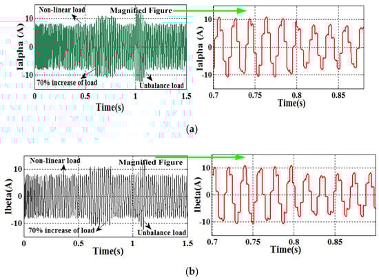
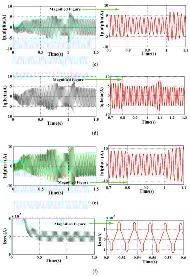
Figure 6.
(a,b) Non-linear load current component, (c,d) active and reactive power components, (e) linear reference active current component produced by combining all grid and load data, and (f) neutral current component.
4.2. System Performance Study during Both Steady and Dynamic States
The load variation time duration in case-2 is like case-1. The total operation of the proposed approach is illustrated in Figure 7. As shown in Figure 7, during 0–0.4 s, the system is operated with no controller. During 0.4–0.6 s, the system performance is tested by using both non-linear and proposed NHCT controllers. In 0.6–0.8 s, the system performance is tested by using a 70% increase in non-linear load and an NHCT controller. During 0.8–1 s, the system performance is tested using both non-linear load NHCT controllers. Finally, during 1–1.1 s, the system performance is studied by unbalancing the load and using an NHCT controller. Finally, during 1.1–1.5 s, the proposed system is tested by using both non-linear load and an NHCT controller. The conventional controller may work efficiently during linear grid voltage and constant balanced load applications. However, in this test condition, for showing the better performance of the proposed NHCT approach over the conventional instantaneous power theory approach, the test condition is planned and tested during distorted grid voltage and a change in non-linear load conditions.
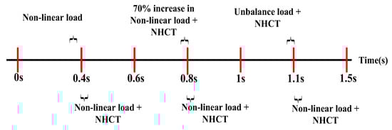
Figure 7.
Working conditions selected for the proposed approach.
Due to the non-linear load, Figure 8a shows that the grid voltage becomes non-linear. A magnified figure is also presented with the original figure for a clear version of Figure 8a. In addition to that, the designed non-linear and unbalanced load model also produces non-linear and unstable current results, as illustrated in Figure 8b. As per the set condition, Figure 8b shows that, during 0–0.6 s, the designed load produces a constant non-linear load current. From 0.6 to 0.8 s, the non-linear load current result suddenly increases to 70% from its rated condition, and at 0.8–1 s, the non-linear load current decreases to its rated limit. To show the transient performance of the proposed controller, the non-linear load is changed to an unbalanced load for a duration of 1–1.1 s, and after 1.1 s, it is changed to a non-linear load and maintains its rated limit. The related variations are stated in Figure 8b. The proposed NHCT tracks the real conditions of the grid voltage and non-linear/unbalanced load condition and generates the harmonic current from the 3φ4W VSI to mitigate the nonlinearity present in the system. The required filter current for harmonic elimination is illustrated in Figure 8c. From the obtained results, it is visualized that the proposed 3φ4W VSI is well capable of producing the required current during variable non-linear and unbalanced load conditions.
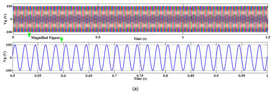
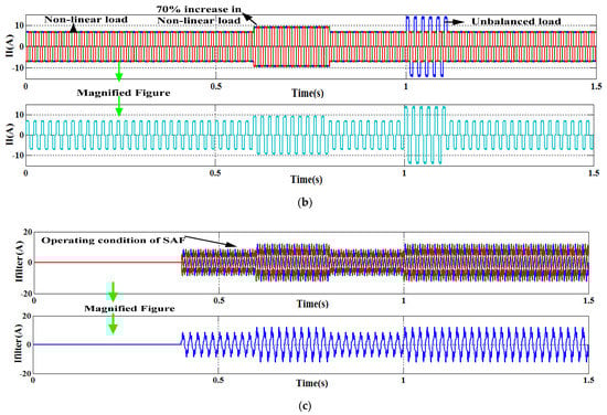
Figure 8.
(a) Grid voltage results, (b) non-linear load current results, and (c) 34W VSI output current results.
Using the traditional p-q-r control approach, the proposed system grid current result is presented in Figure 9a at the change in load condition. As shown in Figure 9a, the grid current results indicate it contains more harmonics than the IEEE/IET standards. The harmonic percentage of the grid current is computed through a Fast Fourier Transform (FFT) analysis technique, and the calculated results are illustrated in Figure 9b(i–iv). Figure 9b(i) shows that, during 0–0.4 s, the grid current contains 30.39% of the harmonics. During that period, the harmonic contained in the grid is equal to the non-linear load harmonic included due to the absence of the controller. Figure 9b(ii) shows that, during 0.4–0.6 s, due to the conventional control approach, the harmonic contained is reduced to 2.95%. Figure 9b(iii) shows that, during the 70% increase in load demand (0.6–0.8 s), the harmonic current-controlled is reduced to 4.2% by using the conventional approach. Figure 9b(iv) shows that, during unbalanced load conditions (1–1.1 s), the harmonic current is reduced to 3.24% by using the traditional strategy. From the above-discussed results, it can be concluded that the developed model suffers from PQ problems, as the grid current contains higher harmonics as per the IEEE/IET standards. Therefore, finding an optimal solution for the proposed non-linear/unbalanced load model is necessary.
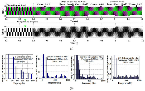
Figure 9.
(a) Traditional grid current results (b) Traditional FFT results.
In the proposed approach, using the NHCT approach, the performance of the non-linear/unbalanced-based undertaken system is tested. From the study, it is found that the 34W VSI injects the required harmonics into the system to mitigate the harmonics. Due to the application of the NHCT approach, the grid current harmonics of the grid current are reduced significantly, as illustrated in Figure 10a. Figure 10a shows that the magnitude of the currents is changed according to the load requirement. For a clear vision of the grid current results, the magnified figure is also presented.
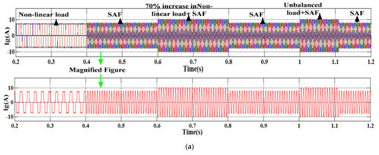

Figure 10.
(a) Proposed grid current results (b) Proposed FFT results.
Similarly, the harmonic containing the grid current using the proposed approach is tested through the FFT analysis. Figure 10b(i) shows that, during the absence of the NHCT controller, the grid current harmonic percentage is equal to the non-linear load current percentage, i.e., 30.39%. Figure 10b(ii) shows that, during the proposed control approach, the grid current harmonic contained is reduced to 0.8%. Figure 10b(iii) shows that, during the 70% increase in load demand, the grid current harmonic percentage is also reduced to 1.39%. In addition to that, the THD result of the grid current is reduced to 1.8% and grid voltage is reduced to 0.02% with the application of non-linear/unbalanced load as illustrated in Figure 10b(iv) and Figure 10b(v) respectively. In addition to that, Therefore, the proposed approach results indicate that the grid current harmonic contained is decreased significantly. From the above analysis, it is proved that, by applying the NHCT approach, the power quality of the proposed 34W system is improved. Therefore, it is suggested to implement the proposed controller for 34W real-time system application.
4.3. Comparative Study
For better justification of the proposed control approach in comparison to conventional P-Q-R strategies, a few comparative results are presented in Figure 11a–e. The magnified version of Figure 11a,b,d is illustrated on the right side of the given figure. Figure 11a shows that, by using both conventional and proposed approaches, the frequency of the operating system is 50 Hz. However, during the load change condition, the notches or settling time of the frequency are higher than the conventional approach. The magnified version of Figure 11a indicates that the frequency response is quite distorted during the traditional procedure compared to the proposed method. Figure 11b shows the neutral current figures obtained during both the conventional and proposed approaches. Using the proposed approach, the neutral current is reduced to a significant value, by which the circulating current and harmonic contained are decreased significantly. Figure 11c shows the results of both power factor (pf) values during both conventional and proposed approaches. Figure 11c indicates that by using the traditional method, the pf of the test system is computed as 0.81. However, Figure 11c suggests that, by using the proposed approach, the pf of the test system is calculated as 0.92. Thus, the spikes produced in the pf results during the sudden load change are more during the conventional approach. In this proposed approach, the dc-link voltage of the converter is regulated and compared with the traditional dc-link voltage, as illustrated in Figure 11d. Figure 11d shows that the peak overshoot and undershoot values of the dc-link voltage are more with the conventional result than with the proposed approach result. Therefore, to settle the dc-link voltage, the traditional approach takes more time than the proposed approach. The magnified version of Figure 11d clearly illustrates that the proposed method provides faster settling time as compared to traditional method. Figure 11e shows the active and reactive power results of the proposed and conventional approaches. By using the traditional approach, Figure 11e shows that the active and reactive power results contain both average and oscillating components.
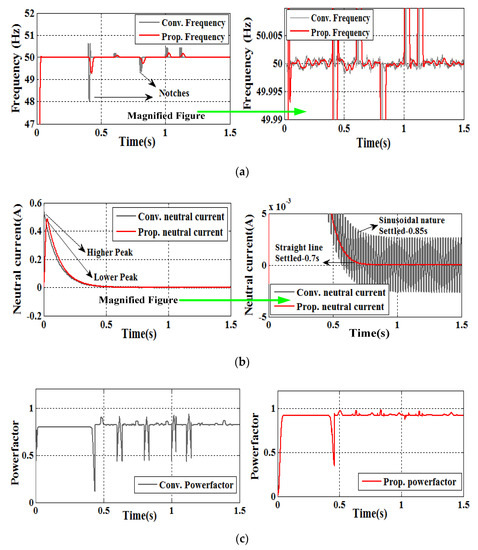
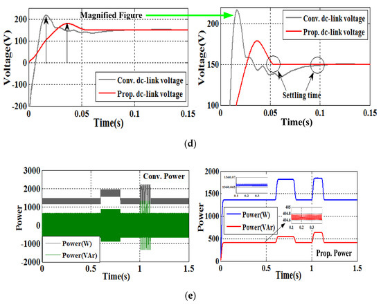
Figure 11.
(a) Frequency response of the system, (b) neutral current result, (c) power factor result, (d) dc-link voltage results, and (e) active and reactive power results.
However, by using the proposed NHCT approach, the three-phase four-wire system generates only the desired average active and reactive power components. By comparing the traditional and proposed power curves, it is visualized that the traditional controller-based inverter is incapable of regulating the reactive power flow. Therefore, the harmonic contained percentage exceeds the acceptable IEEE limit and it is not recommended for real-time application. By using the proposed NHCT approach, the three-phase four-wire system generates appropriate reactive power and compensates the harmonic significantly as per the prescribed limit. Figure 11e illustrates that, at 0–0.6 s, the inverter generates 405 Var with a constant load; at 0.6–0.8, the inverter generates 510 Var with an increase in load; at 0.8–1 s, the inverter generates again 405 Var with a constant load; at 1–1.1 s, the inverter increases the reactive power to 600 Var with unbalanced load applications; and at 1.1–1.5 s, the inverter again decreases the reactive power supply to 405 Var with a constant load application. The above Var result indicates that the proposed system regulates the reactive power supply and harmonic significantly as compared to the traditional approach. As per the above comparative results, it is suggested to operate the proposed 34W system by using the proposed NHCT approach.
By analyzing the above case studies, and for a quantitative relative representation, Table 1 is presented. In Table 1, the analysis is performed by computing the THD% and settling time of the obtained signal. Table 1 indicates that, due to the proposed approach, the harmonic percentage is significantly reduced to a standard value. In the presented Table 1, the harmonic mitigation ratio (HMR) percentage and improvement percentage (IP) are additionally computed for making a clear vision of the proposed control strategy. The HMR percentage and improvement percentage are calculated using a mathematical formula as shown in Equations (26) and (27).

Table 1.
Comparative study.
Using Equations (26) and (27), the performance of the proposed NHCT approach is studied, and the computed quantitative values are presented in Table 1. As per the computation, HMR% is varied in between 2.5% and 5.5%. This indicates that the proposed controller is efficient enough to control any certain dynamic changes in the system. In addition to that, the improvement percentage also shows that, by using the proposed NHCT strategies, the system’s performance is improved significantly. The harmonic contained in the neutral current is more during the conventional approach application. However, by using the proposed NHCT approach, the harmonic contained is reduced to zero. Therefore, the proposed strategy applies to real-time/industrial applications.
5. Conclusions
This manuscript presents a robust 34W SAF control technique to increase the performances of the 34W systems under different conditions such as non-linear load, unbalanced load, and specifically distorted grid voltage conditions. From the above study, it is found that the test system can significantly regulate the circulating current in between the system by using the proposed approach. Due to the above factor, the PQ and computational burden of the system is improved. The effectiveness of the suggested NCVC and NHCT approach is verified through MATLAB/Simulink software at different time intervals. The simulated outcomes prove that the following objectives can be attained during unbalanced/non-linear load and non-linear grid voltage conditions.
- Harmonic current compensation.
- Providing appropriate reactive power support.
- Reducing the excess neutral current
- Regulating the harmonics of the grid current.
- Better frequency trackability.
- Improving the power factor of the system nearer to unity.
- Better dc-link voltage regulation.
As per the IEEE Std.1459- 519 and MIL-STD-704E, the proposed NHCT approach performs well within the specific harmonic limit by considering a 34W SAF with zero sequence components. The above-obtained results show that, by using the proposed approach, the overall percentage of HMR and improvement percentage of THD are computed as 4.14% and 66.78%, respectively, at different test conditions. From Table 1, it is found that the HMR percentage lies well within the prescribed IEEE limit, and the overall THD percentage is improved significantly compared to the traditional approach. That indicates the proposed method effectively works during dynamic real-time conditions. However, the 34W-based grid-integrated non-linear test system still requires further hardware verifications due to measurement mistakes. The possibility of mismatch rises because of measurement sensors and the system parameters such as the line parameters and transformer impedances and switching parameters. To resolve the above issues, good-quality instruments having maximum precision and improved protection strategies are used. In this suggested approach, the attained and examined simulated results serve as a basis of a robust NHCT control approach for the non-linear/unbalanced-load-based 34W system on real-time applications.
Author Contributions
Conceptualization, B.S.; methodology, B.S.; software, B.S.; validation, B.S., M.M.A. and P.K.R.; formal analysis, B.S.; investigation, B.S.; resources, B.S.; data curation, B.S.; writing—original draft preparation, B.S.; writing—review and editing, B.S.; visualization, B.S.; supervision, B.S.; project administration, B.S.; funding acquisition, M.M.A. All authors have read and agreed to the published version of the manuscript.
Funding
This research received no external funding.
Data Availability Statement
Not applicable.
Acknowledgments
The authors acknowledge the support provided by the Silicon Institute of Technology, Sambalpur.
Conflicts of Interest
The authors declare no conflict of interest.
Appendix A. Filter Design
- (i)
- Design and use of the Notch Filter
In this proposed approach, a standard-type notch filter () is considered for eliminating the higher-order harmonics present in the voltage and current signal. A second-order filter is considered for designing the control model and eliminating the distortion factor present in the circuit. The undertaken second-order system parameter is given below [34,35].
For computing the notch frequency, the following points are necessary to follow.
- (1)
- Guess an initial excitation frequency .
The input current/voltage signals R(s) can be exhibited as a pure cosine function described by . By considering the above function, the steady-state equation can be computed as
- (2)
- Compute the amplitudes B1(1) and B2(1) using the system dynamics.
From the above Equations (A3) and (A4), the magnitude of the output signal ‘B’ can be computed as
For simplicity, Equation (A5) can be further simplified as follows.
From Equation (A6), if we choose an excitation frequency that is smaller than the notch frequency, then we can ignore the absolute sign and solve for to yield an explicit solution for as follows.
If we choose an excitation frequency that is larger than the notch frequency, then we can replace the absolute sign with a negative sign and solve for to yield an explicit solution for as follows.
- (3)
- Compute the new excitation frequency using Equation (A9) when k = 2.
- (4)
- Repeat the following until is small:
- (a)
- Compute the amplitudes B1(k − 1) and B2 (k − 1) using the system dynamics.
- (b)
- Compute the new excitation frequency using Equation (A9).
When getting closer to the notch frequency, the term should be decreased to a small value. That means that, when the excitation frequency gets closer to the notch frequency, the successive changes in Equation (A9) only vary within two values of the excitation frequency.
Obtained results:
To ensure the linear relationship between the dynamic and static responses, the range of is selected as 0.8. By putting the obtained notch values in Equation (A1), the notch filter is designed and applied for non-linearity elimination, as illustrated in Figure 2. After determining the notch frequency ( rad/s), the Bode plot of the second-order filter can be evaluated and illustrated in Figure A1a below. As shown in Figure A1a, the developed second-order notch filter provides a 20 dB attenuation at a frequency of 10 rad/s. The Bode plot results show that the filter design offers a stable response and is applicable for real-time applications. Generally, the control system components are designed in a continuous-time interval. However, looking at real-time applications such as digital computers and embedded processors, converting them into a discretized form is necessary. To discretize the continuous-time systems, several discretization algorithms, Zero-order holds, First-order hold, Impulse invariant, Tustin (bilinear approximation), Tustin with frequency pre-warping, Matched poles, and zeros, are supported by Control System Toolbox. Using the above methods, the comparative Bode plot results of the developed notch filter are studied and illustrated in Figure A1b. As illustrated in Figure A1b, the system offers the most accurate frequency-domain approximation of the notch filter by using the matched poles and zero discretization algorithm. The comparative Bode, as well as filtered sine wave results, are illustrated in Figure A2. Due to the discretization algorithm, it is easier to compute a more linearized response as compared to the continuous-time signals. The Bode results as illustrated in Figure A1b and Figure A2 show that, by using the selected discretize algorithm, the system offers faster filtering action.
- (ii)
- Use of Inductive and Capacitive Filter
Inductive and capacitive filters are nothing but passive filters. They are used to eliminate the higher-frequency and low-frequency unwanted components present in the system. The behavior of the passive filter as an inductive and capacitive filter is decided by the nature of the frequency. The related conditions are illustrated below. These filters are not different from each other, but, according to the situation, the inductive and capacitive operations are decided. For a general representation, and to obtain a clear mathematical expression, in Figure 2, inductive and capacitive filters are separately presented. According to the situation, the nature and behavior of the filter are decided.
- At a frequency below the resonant frequency i.e., f < f0, XL >> XC. Hence, the circuit is inductive.
- At a frequency above the resonant frequency i.e., f > f0, XC >> XL. Hence, the circuit is capacitive.
- At a resonant frequency i.e., f = f0, XL = XC, the current is at minimum, and impedance is at maximum. In this state, the circuit can act as a rejector circuit.
- Noise filter
As the system is integrated with both nonlinear and unbalanced loads, then the system performance is affected due to the presence of additional disturbance signals (noise) in the circuit. Therefore, looking at the present need and eliminating the disturbances, a noise filter is used for the controller design. It is capable of handling high-frequency signals in the MHz range by eliminating them and passing the desired signal.

Figure A1.
(a) Bode plot result of the notch filter. (b) Discretized comparative bode plot results.

Figure A2.
Bode plot and filter sine wave result at the notch frequency.
Appendix B. System Parameters
Table A1.
System parameters.
Table A1.
System parameters.
| Parameters | Synonyms | Values |
|---|---|---|
| Grid Voltage | (Phase) | 100 V, 50 Hz |
| Sampling Frequency | 10 kHz | |
| Switching Frequency | 10 kHz | |
| Notch Filter | rad/s | |
| Noise Filter in current regulator loop | ||
| Noise Filter time constant in the active power droop regulator | 1 ms | |
| Active power regulator gain | ||
| Frequency regulator gain | ||
| Active power frequency droop coefficient | 0.08333 Hz/MW | |
| SAF current regulator | PI regulator (s) | |
| Point of common controlling voltage regulator | PI regulator (s) | 5.0 |
| Regulator for PLL | 20.0 | |
| Shunt active filter | ||
| Inductor Filter | ||
| Filter capacitor | ||
| Switch Resistance | ||
| Capacitor dc-link voltage | ||
| Non-linear Load Parameter | ||
| -Thyristor controlled rectifier (abc) | ||
| -diode rectifier (bn) | ||
| -diode rectifier (cn) | ||
References
- Murshid, S.; Singh, B. Utility Grid Interfaced Solar WPS Using PMSM Drive with Improved Power Quality Performance for Operation under Abnormal Grid Conditions. IEEE Trans. Ind. Appl. 2019, 56, 1052–1061. [Google Scholar] [CrossRef]
- Sahoo, B.; Routray, S.K.; Rout, P.K. Repetitive control and cascaded multilevel inverter with integrated hybrid active filter capability for wind energy conversion system. Eng. Sci. Technol. Int. J. 2019, 22, 811–826. [Google Scholar] [CrossRef]
- Singh, A.K.; Kumar, S.; Singh, B. Solar PV Energy Generation System Interfaced to Three Phase Grid with Improved Power Quality. IEEE Trans. Ind. Electron. 2019, 67, 3798–3808. [Google Scholar] [CrossRef]
- Liang, X. Emerging power quality challenges due to integration of renewable energy sources. IEEE Trans. Ind. Appl. 2016, 53, 855–866. [Google Scholar] [CrossRef]
- Sahoo, B.; Routray, S.K.; Rout, P.K. Integration of wind power generation through an enhanced instantaneous power theory. IET Energy Syst. Integr. 2020, 2, 196–206. [Google Scholar] [CrossRef]
- Javadi, A.; Woodward, L.; Al-Haddad, K. Real-time implementation of a three-phase THSeAF based on a VSC and a P + R controller to improve the power quality of weak distribution systems. IEEE Trans. Power Electron. 2017, 33, 2073–2082. [Google Scholar] [CrossRef]
- Tian, H.; Li, Y.W.; Zhao, Q. Multirate Harmonic Compensation Control for Low Switching Frequency Converters: Scheme, Modeling, and Analysis. IEEE Trans. Power Electron. 2019, 35, 4143–4156. [Google Scholar] [CrossRef]
- Sahoo, B.; Routray, S.K.; Rout, P.K. Artificial Neural Network-Based PI-Controlled Reduced Switch Cascaded Multilevel Inverter Operation in Wind Energy Conversion System with Solid-State Transformer. Iran. J. Sci. Technol. Trans. Electr. Eng. 2019, 43, 1053–1073. [Google Scholar] [CrossRef]
- Sahoo, B.; Routray, S.K.; Rout, P.K. A novel control strategy based on hybrid instantaneous theory decoupled approach for PQ improvement in PV systems with energy storage devices and cascaded multilevel inverter. Sādhanā 2020, 45, 13. [Google Scholar] [CrossRef]
- Ye, J.; Gooi, H.B.; Zhang, X.; Wang, B.; Pou, J. Simplified Four-Level Inverter-Based Dynamic Voltage Restorer with Single DC Power Source. IEEE Access 2019, 7, 137461–137471. [Google Scholar] [CrossRef]
- Jou, H.-L.; Wu, K.-D.; Wu, J.-C.; Li, C.-H.; Huang, M.-S. Novel power converter topology for three-phase four-wire hybrid power filter. IET Power Electron. 2008, 1, 164–173. [Google Scholar] [CrossRef]
- Sahoo, B.; Routray, S.K.; Rout, P.K. Execution of robust dynamic sliding mode control for smart photovoltaic application. Sustain. Energy Technol. Assess. 2021, 45, 101150. [Google Scholar] [CrossRef]
- Su, X.; Masoum, M.A.; Wolfs, P. Comprehensive optimal photovoltaic inverter control strategy in unbalanced three-phase four-wire low voltage distribution networks. IET Gener. Transm. Distrib. 2014, 8, 1848–1859. [Google Scholar] [CrossRef]
- Bhosale, S.S.; Bhosale, Y.N.; Chavan, U.M.; Malvekar, S.A. Power Quality Improvement by Using UPQC: A Review. In Proceedings of the 2018 International Conference on Control, Power, Communication and Computing Technologies (ICCPCCT), Kannur, India, 23–24 March 2018; pp. 375–380. [Google Scholar]
- Sahoo, B.; Routray, S.K.; Rout, P.K. AC, DC, and hybrid control strategies for smart microgrid application: A review. Int. Trans. Electr. Energy Syst. 2020, 31, e12683. [Google Scholar] [CrossRef]
- Ni, F.; Li, Z.; Wang, Q. The Voltage Control Strategy of a DC-Link Bus Integrated Photovoltaic Charging Module in a Unified Power Quality Conditioner. Energies 2019, 12, 1842. [Google Scholar] [CrossRef]
- Jarwar, A.R.; Soomro, A.M.; Memon, Z.A.; Odhano, S.A.; Uqaili, M.A.; Larik, A.S. High dynamic performance power quality conditioner for AC microgrids. IET Power Electron. 2019, 12, 550–556. [Google Scholar] [CrossRef]
- Sahoo, B.; Routray, S.K.; Rout, P.K. Hybrid generalised power theory for power quality enhancement. IET Energy Syst. Integr. 2020, 2, 404–414. [Google Scholar] [CrossRef]
- Zhang, H.; Da Sun, C.; Li, Z.-X.; Liu, J.; Cao, H.-Y.; Zhang, X. Voltage vector error fault diagnosis for open-circuit faults of three-phase four-wire active power filters. IEEE Trans. Power Electron. 2016, 32, 2215–2226. [Google Scholar] [CrossRef]
- Sahoo, B.; Routray, S.K.; Rout, P.K. Application of mathematical morphology for power quality improvement in microgrid. Int. Trans. Electr. Energy Syst. 2020, 30, e12329. [Google Scholar] [CrossRef]
- Kumar, M.; Srivastava, S.C.; Singh, S.N. Control strategies of a DC microgrid for grid connected and islanded operations. IEEE Trans. Smart Grid 2015, 6, 1588–1601. [Google Scholar] [CrossRef]
- Sahoo, B.; Routray, S.K.; Rout, P.K. Advanced Speed-and-current control approach for dynamic electric car modelling. IET Electr. Syst. Transp. 2021, 11, 200–217. [Google Scholar] [CrossRef]
- Villalva, M.G.; Gazoli, J.R.; Filho, E.R. Comprehensive approach to modeling and simulation of photovoltaic arrays. IEEE Trans. Power Electron. 2009, 24, 1198–1208. [Google Scholar] [CrossRef]
- Sahoo, B.; Routray, S.K.; Rout, P.K. Complex dual-tree wavelet transform and unified power management based control architecture for hybrid wind power system. Sustain. Energy Technol. Assess. 2021, 47, 101560. [Google Scholar] [CrossRef]
- Li, Y.; Vilathgamuwa, D.; Loh, P.C. Microgrid power quality enhancement using a three-phase four-wire grid-interfacing compensator. IEEE Trans. Ind. Appl. 2005, 41, 1707–1719. [Google Scholar] [CrossRef]
- de Almeida Carlos, G.A.; Jacobina, C.B.; dos Santos, E.C. Alternative Breed of Three-Phase Four-Wire Shunt Compensators Based on the Cascaded Transformer with Single DC Link. IEEE Trans. Ind. Appl. 2018, 54, 2492–2505. [Google Scholar] [CrossRef]
- Sahoo, B.; Routray, S.K.; Rout, P.K. A novel sensorless current shaping control approach for SVPWM inverter with voltage disturbance rejection in a dc grid–based wind power generation system. Wind. Energy 2020, 23, 986–1005. [Google Scholar] [CrossRef]
- Tareen, W.U.K.; Mekhielf, S. Three-phase transformerless shunt active power filter with reduced switch count for harmonic compensation in grid-connected applications. IEEE Trans. Power Electron. 2018, 33, 4868–4881. [Google Scholar] [CrossRef]
- Ufnalski, B.; Kaszewski, A.; Grzesiak, L.M. Particle Swarm Optimization of the Multioscillatory LQR for a Three-Phase Four-Wire Voltage-Source Inverter With an LC Output Filter. IEEE Trans. Ind. Electron. 2014, 62, 484–493. [Google Scholar] [CrossRef]
- Sahoo, B.; Routray, S.K.; Rout, P.K. Robust control approach for stability and power quality improvement in electric car. Int. Trans. Electr. Energy Syst. 2020, 30, e12628. [Google Scholar] [CrossRef]
- Panigrahi, R.; Subudhi, B.; Panda, P.C. A robust LQG servo control strategy of shunt-active power filter for power quality enhancement. IEEE Trans. Power Electron. 2015, 31, 2860–2869. [Google Scholar] [CrossRef]
- Sahoo, B.; Routray, S.K.; Rout, P.K.; Alhaider, M.M. Power quality and stability assessment of hybrid microgrid and electric vehicle through a novel transformation technique. Sustain. Energy Technol. Assess. 2022, 51, 101927. [Google Scholar] [CrossRef]
- Merritt, N.R.; Chakraborty, C.; Bajpai, P. New voltage control strategies for VSC-based DG units in an unbalanced microgrid. IEEE Trans. Sustain. Energy 2017, 8, 1127–1139. [Google Scholar] [CrossRef]
- Pogaku, N.; Prodanovic, M.; Green, T.C. Modeling, analysis and testing of autonomous operation of an inverter-based microgrid. IEEE Trans. Power Electron. 2007, 22, 613–625. [Google Scholar] [CrossRef]
- Sahoo, B.; Routray, S.K.; Rout, P.K. Robust control approach for the integration of DC-grid based wind energy conversion system. IET Energy Syst. Integr. 2020, 2, 215–225. [Google Scholar] [CrossRef]
- Merritt, N.R.; Chakraborty, C.; Bajpai, P. control strategy for islanded operation of a Voltage Source Converter (VSC) based distributed resource unit under unbalanced conditions. In Proceedings of the 2015 IEEE 13th International Conference on Industrial Informatics (INDIN), Cambridge, UK, 22–24 July 2015. [Google Scholar]
- He, S.; Song, J.; Liu, F. Robust finite-time bounded controller design of time-delay conic nonlinear systems using sliding mode control strategy. IEEE Trans. Syst. Man Cybern. Syst. 2017, 48, 1863–1873. [Google Scholar] [CrossRef]
- Maccari, L.A.; Amaral Santini, C.L.D.; Pinheiro, H.; de Oliveira, R.C.; Montagner, V.F. Robust optimal current control for grid-connected three-phase pulse-width modulated converters. IET Power Electron. 2015, 8, 1490–1499. [Google Scholar] [CrossRef]
- Sahoo, B.; Routray, S.K.; Rout, P.K. A new topology with the repetitive controller of a reduced switch seven-level cascaded inverter for a solar PV-battery based microgrid. Eng. Sci. Technol. Int. J. 2018, 21, 639–653. [Google Scholar] [CrossRef]
- Vodyakho, O.; Mi, C.C. Three-level inverter-based shunt active power filter in three-phase three-wire and four-wire systems. IEEE Trans. Power Electron. 2009, 24, 1350–1363. [Google Scholar] [CrossRef]
- Sahoo, B.; Routray, S.K.; Rout, P.K. A novel centralized energy management approach for power quality improvement. Int. Trans. Electr. Energy Syst. 2020, 31, e12582. [Google Scholar] [CrossRef]
- Zajkowski, K. Two-stage reactive compensation in three-phase four-wire systems at non-sinusoidal periodic waveforms. Electr. Power Syst. Res. 2020, 184, 106296. [Google Scholar] [CrossRef]
- Routray, S.K.; Sahoo, B.; Dash, S.S. A Novel Control Approach for Multi-level Inverter-Based Microgrid. In Advances in Electrical Control and Signal Systems; Springer: Singapore, 2020; pp. 983–996. [Google Scholar]
- Hirano, K.; Nishimura, S.; Mitra, S. Design of digital notch filters. IEEE Trans. Commun. 1974, 22, 964–970. [Google Scholar] [CrossRef]
- Dutta Roy, S.C.; Kumar, B.; Jain, B.S. FIR notch filter design—A review. Facta Univ.-Ser. Electron. Energetics 2001, 14, 295–327. [Google Scholar]
- Yazdani, A.; Iravani, R. A unified dynamic model and control for the voltage-sourced converter under unbalanced grid conditions. IEEE Trans. Power Deliv. 2006, 21, 1620–1629. [Google Scholar] [CrossRef]
- Sahoo, B.; Routray, S.K.; Rout, P.K. Robust control and inverter approach for power quality improvement. In Green Technology for Smart City and Societ; Springer: Singapore, 2021; pp. 143–156. [Google Scholar]
- Suh, Y.; Lipo, T. Modeling and analysis of instantaneous active and reactive power for PWM AC/DC converter under generalized unbalanced network. IEEE Trans. Power Deliv. 2006, 21, 1530–1540. [Google Scholar] [CrossRef]
Publisher’s Note: MDPI stays neutral with regard to jurisdictional claims in published maps and institutional affiliations. |
© 2022 by the authors. Licensee MDPI, Basel, Switzerland. This article is an open access article distributed under the terms and conditions of the Creative Commons Attribution (CC BY) license (https://creativecommons.org/licenses/by/4.0/).