Article

A Novel Dynamic Approach to Cost-Optimal Energy Performance Calculations of a Solar Hot Water System in an nZEB Multi-Apartment Building

Department of Applied Thermodynamics, Thermal and Process Engineering, Faculty of Mechanical Engineering and Naval Architecture, University of Zagreb, 10002 Zagreb, Croatia
*
Author to whom correspondence should be addressed.
Energies 2022, 15(2), 509; https://doi.org/10.3390/en15020509
Submission received: 10 December 2021 / Revised: 4 January 2022 / Accepted: 6 January 2022 / Published: 11 January 2022

Abstract

:
This paper presents the methodology for conducting a cost-optimal energy performance calculation of a solar hot water system, used for space heating and domestic hot water needs. The calculation is based on dynamic hourly methods, according to the new Energy Performance of Buildings’ (EPB) set of standards EN 15316:2017, and a revision of the standard EN 15316-5:2017 from the year 2021, dealing with storage-tank water temperature calculations. The paper provides proposals for modifications to these newly introduced standards, in order to overcome the observed ambiguities and shortcomings. The calculation of annual energy performance of a building was performed on an hourly basis over a year for the reference of an nZEB multi-apartment building, for a climate area of the city of Zagreb, taking into account water temperature change in the layers of the storage tank connected to solar collectors and hot water boilers. The cost-optimal solution was then determined by varying individual parameters of the building technical system. The influence of these parameters on the energy efficiency of the building was analyzed in detail. Furthermore, the results were compared against those obtained by the Croatian calculation algorithm based on the previous set of EPB standards, EN 15316:2008, currently used EU-wide for the energy performance certification of buildings. The results indicated that the calculation methods of the present algorithm underestimated the consumption of building primary energy by 12%. The energy delivered by solar collectors was underestimated by 18%.

Graphical Abstract

1. Introduction

In the context of tackling climate change and a possible energy crisis, the European Union (EU) has recognized that a significant share of CO2 emissions (36%) and energy consumption (40%) in Europe can be attributed to the building sector [1]. Consequently, the EU has adopted a legislative framework that includes the first recast of the Energy Performance of Buildings Directive, 2010/31/EU (EPBD), and the Energy Efficiency Directive 2012/27/EU (EED). The goal of these directives was to promote the energy efficiency and decarbonization of buildings. One of the EPBD recast key requirements was that all new buildings by 31 December 2020 (31 December 2018 for public buildings) should be nearly zero-energy buildings (nZEBs). An nZEB is defined as a building that is highly energy efficient, with almost zero or a very low amount of required energy, which should be covered to a very significant extent by renewable energy sources (RES) [2].
When designing nZEBs, the cost-effectiveness of building elements and their technical systems should be considered. The cost-optimal energy efficient nZEB design is the result of an optimal interaction between energy demand, energy supply and financial cost. In that regard, a calculation procedure of the cost-optimal analysis has been established according to EU regulations [3]. The comparative methodology of cost-optimal analysis, described in the guidelines [4] supplementing regulation, is used to compare different design alternatives. In short, investment and operation costs (for the period of the estimated building renovation cycle) are determined for different design solutions, and the global cost is calculated for each. The solution with the lowest global cost is declared as the optimal building design.
The complexity of such an approach has prompted the development of computer-based simulation and optimization methods. By combining a building performance simulation software (BPS) with an optimization engine, it is possible to find a cost-optimal solution quickly and inexpensively. This computer-automated process allows any number of building parameters to be varied at the same time. In an effort to shorten the calculation time and reduce computational effort, only a few significant parameters are usually varied. Such an approach allows the determination of the building’s proper design and its technical system configuration, as well as prevention of over- or under-sizing of the system.
The advantage of computer-aided simulation and optimization was demonstrated as early as 1976, when Wilson and Templeman [5] presented a method for determining an optimal thermal design for an office building. Since then, BPS and optimization tools have become widely available. In the literature, the most common software used for detailed dynamic building simulation are TRNSYS (Solar Energy Laboratory, UW-Madison), IDA ICE (EQUA Simulation AB) and EnergyPlus (U.S. Department of Energy). Mazzeo et al. [6] compared simulation results obtained from those BPSs against the real measured data, operating under real conditions. The comparison, carried out on the small-scale solar test boxes, showed relatively high overall accuracy in the prediction of operating conditions. In the open literature, MATLAB (MathWorks Inc., Natick, MA, USA) and GenOpt (U.S. Department of Energy) are most commonly used for optimization purposes. Listed software can be used for determining the optimal level of energy demand [7,8], the optimal level of energy supply [9,10], or both [11,12]. As presented by Ferrara et al. [13] a considerable number of additional studies concerning the use of simulation-based optimization software in nZEB design are available. In this paper, authors acknowledge that, in addition to detailed dynamic simulations, simplified and standardized methods for calculating the building’s energy needs, such as the quasi-steady state monthly method, or the simple hourly method defined by the European Committee for Standardization (CEN) in EN ISO 13790:2008, are also used in practice. In order to assess a building’s technical system energy requirements and efficiency, the results obtained by those methods can be directly linked to the calculation procedure based on the EN 15316:2008 standard series, providing EPBD complying methods for determining delivered and primary energy. Although detailed dynamic simulations provide more comprehensive and precise hourly calculations, such simulations require additional computational power, and are usually associated with high software cost and a steep learning curve, which renders them impractical for everyday use. Moreover, due to non-standardized input data and methodology, the results between individual projects are not comparable to the desired level. In contrast, the previously mentioned simplified methods (EN ISO 13790:2008 and EN 15316:2008 standard series) are less accurate, due to the errors introduced in order to ease the application, speed up calculation, and standardize the input data. On the other hand, these methods can be easily implemented into an expert own-calculation tool for energy performance evaluation (e.g., spreadsheet calculations). Moreover, numerous cheap or even free commercial tools are available on the market. Furthermore, these methods are, in general, compliant with national methodologies which are more or less harmonized with European Standards. Therefore, in addition to the early stages of building design, these methods can also be used to obtain building Energy Performance Certificates (EPCs).
The evolution of standardized procedure started with the first set of European Standards, developed by CEN and published between 2007 and 2008 (EN ISO 13790:2008, series of standards EN 15316:2008 et al.). This set of forty standards was designed to implement the first EPBD 2002/91/EC. Its application has been shown to be difficult due to the variable quality of individual modules and inadequately described interconnections. Berković-Šubić et al. [14] presented calculation methods implemented into Croatian Algorithms for calculating the energy performance of a building based on the standards EN ISO 13790:2008 and EN 15316:2008, and proved that overwhelming parts of available methods from standards can be successfully applied if certain improvements and modifications to the original calculation procedure are applied. Horvat and Dović [15] compared the results obtained by these methods to those obtained with their own developed dynamic model, and differences of up to 33% were found in the analysis of individual subsystems. The comparison was conducted on the well-insulated single-family house located in the Zagreb area. Vujnović and Dović [16] compared the results of energy performance calculations of the reference nZEB hotel performed by a detailed dynamic simulation in IDA ICE and MGIPU Energetski Certifikator (RH—Ministarstvo prostornoga uređenja, graditeljstva i državne imovine), a government-approved software based on Croatian algorithms. The authors showed that the calculated gap between energy need for heating was only 5%, but the gap between the energy need for cooling was as high as 50%. Although the error introduced by simplified standardized procedures proved to be almost negligible in the case of existing buildings, the same error can be significant in the case of nZEBs, as shown by the present literature review. Therefore, after the EPBD recast, the European Commission decided for CEN to revise these standards. The new set of standards, published in 2017, contains the common modular framework and revised, consistent calculation methods, which now involve hourly time steps, designed for easy implementation in BPS software. Although a revision was conducted, some ambiguities and shortcomings in the new standards can still be found. Nevertheless, more detailed models and hourly calculations should allow for obtaining more precise and accurate results of the energy performance of buildings compared with the previous version of standards. Many studies have been conducted investigating the application of the standard EN ISO 52016-1:2017 [17,18,19,20,21], for dynamic calculations of the building energy needs for heating and cooling. On the other hand, only a few studies have been published by date on the new set of EN 15316:2017 standards, which are intended for calculating the energy efficiency of technical systems in buildings (energy supply). In [22] a novel calculation method for assessing heat emission losses is shown, which complements the standard EN 15316-2:2017. This model, based on the operative temperature, is used to calculate product-specific values of setpoint variations, which are then used in heat loss calculations instead of tabulated values. Piana et al. [23] have shown that EN 15316-4-3:2017 and EN 15316-5:2017 can successfully be applied in the design process of a solar thermal system. In their work, a non-invasive solar loop pump control model, allowing the quantification of the risk of stagnation resulting from increased solar field areas or decreased storage volume, is added to the standard framework.
The reviewed studies usually deal with individual modules [22,23,24,25], but there were no studies found in which the overall calculation was performed with the goal of finding a cost-optimal solution. Hence, the main novelty of this study is in demonstrating the applicability and reliability of the overall complex and comprehensive calculation procedure, based on the new EPB standards for assessing the energy performance of a building. The objective of this study is to show that the new standards, with a few added enhancements and propositions for overcoming detected ambiguities and shortcomings, can be easily interconnected and implemented in a computer code, and applied both to determine the cost-optimal level of energy efficiency, and to size the technical system.
In this paper, simulations of the energy performance of the selected technical system solutions were performed using a dynamic hourly method based on the new set of EPB standards EN 15316:2017, and a revision of the standard EN 15316-5:2017 from 2021 (prEN 15316-5:2021). A simple economic analysis and an automated optimization method were used to determine the cost-optimal system solution. These calculation procedures are described in Section 2. A case study was conducted on a reference nZEB multi-apartment building in the continental part of Croatia. The focus was placed on optimizing the solar-assisted system, which is used for space heating (SH) and the preparation of domestic hot water (DHW). The input data of the building and the system used in calculations are given in Section 3. The analysis of the results of cost-optimal energy performance calculations, as well as the comparison of the results between the new (hourly calculations) and old version (monthly calculations) of the EPB standards, are presented in Section 4. Finally, Section 5 provides conclusions and recommendations for future research.

2. Methodology

2.1. Energy Performance Simulation according to Standard Series EN 15316:2017

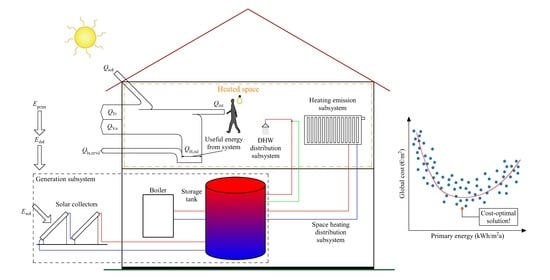
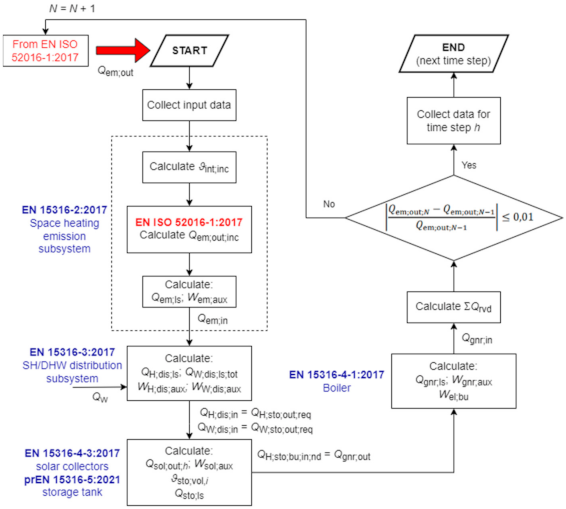
This chapter provides an overview of the calculation methods based on the set of EPB standards EN 15316:2017 for assessing the energy performance of a solar hot water system used for SH and DHW needs, as shown in Figure 1. The calculation procedure starts with the calculation of energy at the output from the subsystem and ends with the calculation of energy input to the subsystem. Each standard describes the method for calculating the heat losses and auxiliary energy consumption of a particular subsystem, according to which the delivered and primary energy of the building are ultimately determined. The calculation flow is shown in Figure 2. The main input data are the energy output from the space heating emission subsystem Qem;out determined according to the standard EN ISO 52016-1:2017 [26] and the energy need for DHW QW determined according to EN 12831-3:2017 [27]. In the following text, basic principles of each standard with proposals to overcome found ambiguities and shortcomings are described.

2.1.1. Space Heating Emission Subsystem

The calculation of the space emission subsystem is performed according to the standard EN 15316-2:2017 [28], which replaces the standard EN 15316-2-1:2007 [29]. Unlike EN 15316-2-1:2007, where the heat losses of the emission subsystem are calculated using the efficiencies method, the calculation procedure in the new version of the standard is based on the calculation of increased indoor air temperature (Equation (1)):
ϑ int ; inc = ϑ int ; ini + Δ ϑ int ; inc ,
where ϑint;ini is initial internal set-point temperature and Δϑint;inc is internal set-point temperature variation calculated as:
Δ ϑ int ; inc = Δ ϑ str + Δ ϑ ctr + Δ ϑ rad + Δ ϑ hydr + Δ ϑ roomaut ,
which takes into account the impact of heat loss due to temperature variation that occurs as a result of non-uniform space temperature distribution ϑstr, control accuracy of indoor temperature ϑctr, radiation ϑrad, hydronic balancing of system ϑhydr and operation of control system ϑroomaut. Calculated ϑint;inc is then used to determine the modified energy at the output from space heating emission subsystem Qem;out;inc, according to [26].
The impact of temperature variation based on additional heating losses of embedded emitters in the building envelope ϑemb is used to calculate the embedded losses Qemb;ls, according to:
Q emb ; ls = Q em ; out ; inc · Δ ϑ emb ϑ int ; inc ϑ e ; comb ,
where ϑe;comb is equal to average outdoor air temperature in observed time step ϑe,avg. Together, Qem;out, Qem;out;inc and Qemb;ls are used to calculate the total heat loss of the emission subsystem:
Q em ; ls = Q em ; out ; inc Q em ; out + Q emb ; ls .
The standard recommends that the operating duration of the fans (operation at nominal power), as well as the operating duration of the control system, should be equal to the operating time of the heating system. The authors of this paper recommend that the fans operating time be calculated as:
t h , rL = Q em ; out Φ Hemn .
This approach, considering only nominal power, does not take into consideration the modulation of the fans’ power. Such an upgrade can be a further improvement of the calculation procedure. Furthermore, the present authors recommend that the auxiliary energy of the control system should be calculated for each hour of the year.

2.1.2. Distribution Subsystem

The calculation of the SH and DHW distribution subsystem is performed according to the standard EN 15316-3:2017 [30], which is a replacement for the standards EN 15316-2-3:2007 [31] and EN 15316-3-2:2007 [32]. The main input data for the SH distribution system is Qem;in (energy input to the emission module) and the main input data for the DHW distribution system is the energy need for DHW QW. The heat loss calculation of a distribution subsystem is based on the mean water temperature, the temperature of space surrounding the pipe section, the thermal transmittance of the pipes, the length of the pipes and the operation time. For the SH distribution system, only heat losses that occur in the circulation loop during the heating system operation are taken into account. For the DHW distribution system, heat losses in the circulation loop are separately calculated for the time when the circulation pump is ON and OFF (if there is a hot water recirculation system), as well as heat losses that occur in open-circuited stubs between subsequent tappings.
According to [30], the heat losses of the SH and DHW circulation loops during circulation pump operating time are calculated according to the same equation:
Q X ; dis ; ls = 0 t X ; op j Ψ j ϑ X ; mean ϑ X ; amb , j · L + L equi j · t ci ,
where j is an index representing pipeline section (zone), Ψj is linear thermal transmittance, ϑX;mean is mean water temperature in the SH/DHW distribution system, ϑX;amb,j is an ambient temperature surrounding the section, L is the length of the pipe section, Lequi is the equivalent length of the pipe section for fittings (valves, tees, bends, etc.), tci is time step of the calculation, and tX;op is the circulation pump operating time. Index X is replaced by H or W in the case of calculating SH or DHW distribution system, respectively.
If the tatap, i.e., time after the last tapping in the tapping profile, or last pump operation in the DHW circulation loop, is known, it is possible to calculate the temperature after the last tapping or last pump operation according to:
ϑ W ; atap , j = ϑ W ; amb , j + ϑ W ϑ W ; amb , j · e Ψ j · L j · t atap c W · ρ W · V W , j + c p · m p , j ,
where ϑW is the design hot water temperature, VW,j is the volume of water in pipe section j, cW is the specific heat capacity of water, ρW is the density of water, cp is the specific heat capacity of the pipes, and mp,j is the mass of pipes. By knowing ϑW;atap,j, the heat loss of the open-circuited stubs, or heat loss of the DHW circulation loop when the pump is not operating, can be calculated as:
Q W ; dis ; nom = 0 t X ; op j Ψ j ϑ W ; avg ϑ X ; amb , j · L + L equi j · t ci
where the average water temperature is:
ϑ W ; avg , j = ϑ W + ϑ W ; atap , j 2 .
If only the number of tapping’s ntap and the volume of water within the pipes is known, the heat loss of the open-circuited stubs QW;dis;stub per time step during tapping can be calculated under the assumption that, between the tappings, the hot water temperature drops to the ambient air temperature according to:
Q W ; dis ; ls ; stub , j = m ˙ W ; dis ; stub · c W · ϑ W ϑ W ; amb , j · t ci ,
where the mass flow of hot water in open-circuited stubs during tapping is given by:
m ˙ W ; dis ; stub = V W , j · ρ W · n tap , j .
If neither the tapping profile nor the pipe dimensions are known, the heat loss of the open-circuited stubs is calculated according to Equation (8), using the simplified method for determining mean water temperature:
ϑ W ; em ; mean = ϑ W ; avg , j = 25 · Ψ j 0.2 .
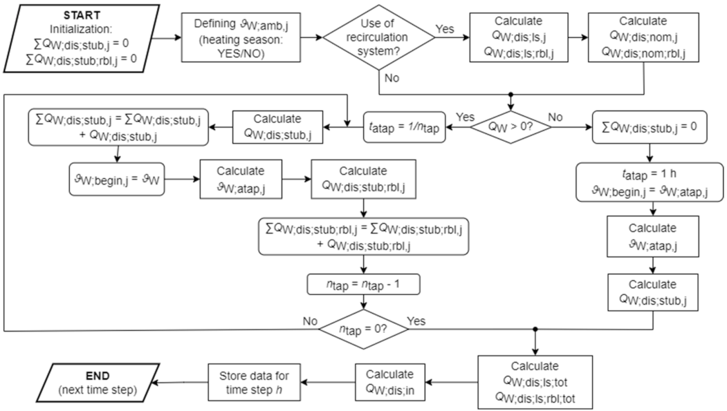
The calculation method of the DHW distribution system heat losses is not clearly described, and it also contains certain shortcomings. According to Equation (8), heat losses of the open-circuited stubs and heat losses of the DHW circulation loop when the pump is not operating are calculated for the period when the pump operates (tW;op). Furthermore, the procedure for obtaining ϑW;atap,j yields questionable results. So, in this paper, a new approach for calculating the heat loss of open-circuited stubs, and the heat loss of the DHW circulation loop when the pump is not operating, is implemented. The calculation flowchart is shown in Figure 3. This method is based on the equality of the heat transfer rate between water and the environment, and the heat transfer rate through the pipe wall. The water temperature after the last pump operation is then calculated according to:
ϑ W ; atap , j = m ˙ W , j · c W · ϑ W 1 t W ; op · Ψ j L + L eq j · ϑ W 2 ϑ W ; amb , j 1 2 1 t W ; op · Ψ j L + L eq j + m ˙ W , j · c W ,
and the water temperature after the last tapping is calculated as:
ϑ W ; atap , j = m ˙ W , j · c W · ϑ W t atap · Ψ j L + L eq j · ϑ W ; begin , j 2 ϑ W ; amb , j 1 2 t atap · Ψ j L + L eq j + m ˙ W , j · c W ,
where the amount of hot water in section j in the observed time step is given by:
m ˙ W , j = V W , j · ρ W 1   h    
and ϑW;begin,j is the water temperature in the pipes at the beginning of the cooling period. If calculated ϑW;atap,j is lower than ϑW;amb,j, then ϑW;atap,j is equal to ϑW;amb,j. If there is tapping in the observed time step, ϑW;begin,j is equal to ϑW, whereas in the case where there is no tapping in the observed time step, ϑW;begin,j is equal to the water temperature at the end of the previous time step ϑW;atap,j;h−1. In this method, time after the last tapping tatap is determined by:
t atap = 1 n tap ,
where ntap represents the number of tappings in the observed time step. Therefore, this method can be used when only the tapping profile is known. Heat losses of the open-circuited stubs during tapping, and heat losses of the DHW circulation loop when the pump is not operating, are calculated according to:
Q W ; dis ; nom = j m ˙ W , j · c W · ϑ W ϑ W ; atap , j · t ci .

2.1.3. Thermal Solar Collectors and Storage Tank

The standard EN 15316-4-3:2017 [33], which supersedes the standards EN 15316-4-3:2007 [34] and EN 15316-4-6:2007 [35], deals with the energy performance calculation of thermal solar collectors and a photovoltaic generation subsystem. Photovoltaic panels were not used in this case study. The standard EN 15316-4-3:2007 describes two methods of monthly calculation of solar thermal system: Method A, which uses system data, and method B (based on the f-chart method), which uses component data. A new dynamic hourly calculation method, based on the energy balance of the solar collector, has been added to the new standard. The new calculation procedure works in conjunction with the storage module (calculation according to the standard prEN 15316-5:2021 [36]). prEN 15316-5:2021 describes two calculation methods. Method A takes into account temperature stratification inside the tank, and it is recommended to use it when analyzing systems with solar collectors. Method B models the storage tank with a uniform temperature and is generally used in all other cases. Temperatures in the storage tank influence the calculation of the heat losses in the solar collectors. This necessitates the iterative calculation in which the convergence condition is described as:
Q sol ; loop ; out ; N Q sol ; loop ; out ; N 1 Q sol ; loop ; out ; N 1 0.05 ,
where Qsol;loop;out is the heat output of collector loop to the storage tank and N is the iteration step. The iteration is executed until the condition is met, or for four times, whereby the fourth iteration is final.
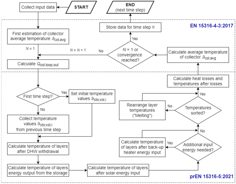
After gathering all the necessary input data, such as meteorological data, hourly loads QH;dis;in and QW;dis;in (output from the distribution module), technical data about solar collectors and storage tanks, and the type of application (SH and/or DHW), the calculation is performed as shown in Figure 4. For each time step, in the initial calculation step, the collector efficiency of 40% is assumed. In the following iteration steps, the collector efficiency ηcol;h is calculated based on the obtained average temperature of the working medium in collector loop ϑcol;avg;h according to:
η col ; h = η 0 · K hem 50 ° a 1 · T h * a 2 · T h * 2 · I sol ; h ,
where η0 is the zero-loss efficiency of the solar collector, Khem(50°) is the incidence angle modifier, a1 and a2 are the first- and second-order heat loss coefficients and T h * is the reduced temperature difference in the collector. Afterwards, the collector output energy is calculated as:
Q sol ; out ; h = η col ; h · I sol ; h · A sol · t ci ,
where Isol;h is the solar irradiance on the collector plane, and Asol is the installed collector area. Finally, the energy output of the collector loop to the storage is calculated by:
Q sol ; loop ; out ; h = Q sol ; out ; h Q sol ; loop ; ls ; h ,
where Qsol;loop;ls;h is heat loss of the collector loop piping. It is important to note that in the case where Qsol;loop;out;h is less than or equal to the power of the collector loop pump multiplied by 3, Qsol;loop;out;h is equal to 0. This takes into account that the working medium temperature in the solar collectors has to rise sufficiently in order for the pump to start. Qsol;loop;out;h is used as input to calculate the storage module.
In addition to the described procedure, the present authors propose a simplified method for checking whether the collector output temperature ϑcol;out;h is equal to or higher than the stagnation set-point temperature ϑstag (e.g., 90 °C). In stagnation, the temperature of the working medium can be calculated as:
ϑ col ; out ; h = ϑ col ; out ; h Q sol ; lstag ; h Q coll ; ls M col · C W ,
with collector stagnation output defined as:
Q sol ; lstag ; h = η col ; h · I sol ; h · A sol · t ci ,
and collector losses calculated as:
Q coll ; ls = A sol a 1 + a 2 · ϑ col ; avg ; h ϑ e ; h · ϑ col ; avg ; h ϑ e ; h ,
where Mcol is the mass of the working medium in the collector, CW is the specific heat of working medium, and ϑe;h is outside air temperature in considered time step. If collector output temperature in the previous time step reaches ϑstag, the pump in the collector loop is switched off, i.e., Qsol;loop;out is equal to 0 in all subsequent time steps, until ϑcol;out;h drops below ϑstag.
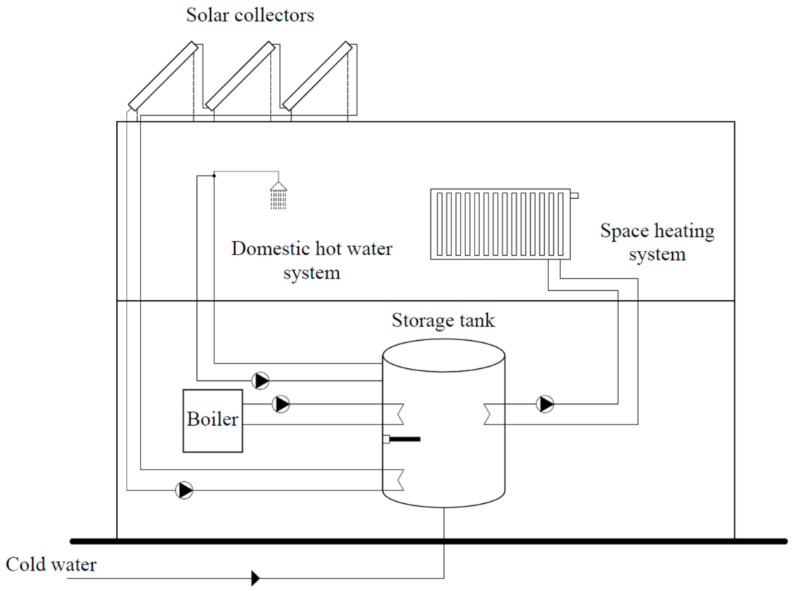
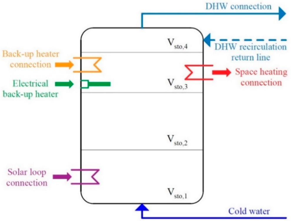
In the case of the solar thermal system with a back-up heater, authors propose using Method A from prEN 15316-5:2021 [36] and dividing the storage unit volume into a minimum of four layers. The schematic of the storage model, including its connections to the rest of the system, is shown in Figure 5. It is important to emphasize that this model, like many others commonly used, assumes that the thickness of the thermocline is zero, to simplify the calculation procedure. Of course, in reality, the thermocline has a certain thickness that changes during operation. A more detailed presentation of the tank model is given in [37]. The calculation method for the storage tank covers the calculation of energy delivered to the storage, i.e., energy delivered by solar collectors and energy delivered by a back-up heater (e.g., combustion boiler, electric heater), energy delivered from the storage to the SH and DHW distribution subsystem, outlet/inlet temperatures from the storage and storage tank heat losses.
The revised standard prEN 15316-5:2021 resolves the ambiguities and shortcomings found in the 2017 version of the standard. This includes the correction of basic energy balances and the ability to define layers of arbitrary volumes. Furthermore, the new version takes into account the contribution of the back-up heater when determining the energy output from the storage, and takes into account the temperature difference between the storage water content temperature, and the working medium temperature in the heat exchanger (if present). The new version of the standards also contains a more precise description of how to consider DHW system losses, the calculation of additional heat losses due to the thermosyphon circulation, and a more accurate definition of heat losses through the envelope of each layer.
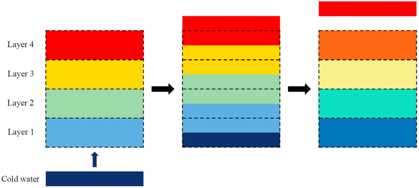
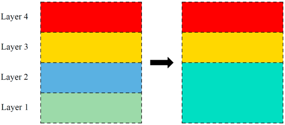
The calculation, based on the energy balance of each layer, is performed by determining the accumulated energy in each layer, defined by the volume of contained water and the temperature difference between the layer temperature and the required temperature. The calculation of the considered time step starts with collecting the temperatures of all layers in the previous time step. After that, the volume withdrawn from storage for DHW service is calculated. Withdrawal is assumed to occur from the top of the storage, while an equal volume of cold water enters the bottom of the storage. All this causes the transport of water through the layer’s boundaries. It is assumed that the water of the upper module is ideally mixed with the quantity of withdrawn water at the temperature of the lower module. This “piston movement” of volume is graphically shown in Figure 6. In the next step, energy withdrawn for the DHW circulation loop is calculated. This is followed by a calculation of the energy withdrawn for SH service. The calculation of energy delivered to the storage by collector loop Qsol;loop;out and back-up heater QH;sto;bu;in;vol,Nvol,bu is then performed. It is important to emphasize that the temperature of each layer is determined after every aforementioned step. When the temperature of the considered layer is higher than the upper layer, then these two layers are melted, as shown in Figure 7. This iterative calculation procedure, according to [36], is maintained until the temperature of the considered layer is lower than or equal to the temperature of the upper layer, i.e., if ϑsto;vol,i > ϑsto;vol,i+1 then:
ϑ sto ; vol , i = ϑ sto ; vol , i + 1 = ϑ sto ; vol , i · V sto ; vol , i + ϑ sto ; vol , i + 1 · V sto ; vol , i + 1 V sto ; vol , i + V sto ; vol , i + 1 ,
where ϑsto;vol is the temperature of the layer, Vsto;vol is the volume of layer, i is the considered layer, and i + 1 is the layer above the considered layer. Standard also describes an alternative approach given in Annex C [36], according to which melting is solved in a defined number of steps (no need for an iterative calculation procedure). After the re-arrangement of the temperatures, thermal losses of each layer and final temperatures are calculated. In the last step, the inlet temperature to the collector loop ϑsol;loop;in and heat generator loop ϑHc;RT are calculated. The calculated ϑsol;loop;in is used to determine ϑcol;avg;h, with which the solar collector is recalculated and the new value of Qsol;loop;out is determined.
It is assumed that the back-up heater in storage operates in ON/OFF mode, and is only turned ON if the temperature of the layer where the heater is placed ϑsto;vol,Nvol,bu is equal to or lower than the defined heater switch-on temperature set-point ϑsto;set;on;bu. Once the heater is turned ON, it should run until all the layers affected by the heater have reached the storage set-point temperature ϑsto;set;on. According to the current procedure within the standard, the heater is turned OFF, even if ϑsto;set;on was not reached in the previous time step. Therefore, the authors of this paper propose an additional condition (condition A) to the equation for determining the total energy need in each layer affected by the back-up heater to increase their temperature to the ϑsto;set;on:
Q H ; sto ; bu ; in ; nd = max i = 2 N vol Q H ; sto ; nd ; in ; vol , i ; 0 for   ϑ sto ; vol , Nvol , bu ϑ sto ; set ; on ; bu max i = 2 N vol Q H ; sto ; nd ; in ; vol , i ; 0 for   C o n d i t i o n   A 0 for   ϑ sto ; vol , Nvol , bu > ϑ sto ; set ; on ; bu ,
with:
C o n d i t i o n   A :   if   and     ϑ sto ; vol , Nvol , bu > ϑ sto ; set ; on ; bu and   ϑ sto ; vol , Nvol , bu ; h 1 < ϑ sto ; set ; on and     Q H ; sto ; bu ; in ; nd ; h 1 > 0 ,
where QH;sto;nd;in;vol,i is the energy to be delivered to each layer to make their temperature equal to ϑsto;set;on, and Nvol is the number of layers used in the model. The notation h represents the observed time step and h − 1 the previous time step. According to this condition, it is checked whether the heater was operational and whether ϑsto;set;on was not achieved in the previous time step. If these two conditions are met, the heater continues to operate in all subsequent time steps until ϑsto;set;on is achieved.

2.1.4. Heat Generation by Fuel Combustion (Boilers)

The standard EN 15316-4-1:2017 [38], which replaces the standards EN 15316-4-1:2008 [39], EN 15316-4-7:2008 [40], and EN 15316-3-3:2007 [41], deals with the energy performance calculation of the water-based heat generation subsystem based on the combustion of fuels (boilers). The new standard unifies the calculation of fossil fuels and renewable fuel boilers and, in addition, redefines the calculation of boilers used for combined service (SH and DHW). In the 2008 version of the standard, calculation of the combined service generator is generally performed for the summed load QHW;gen;out. This increased load QHW:gen;out is then used to determine the generator load factor βgnr which is used to calculate the generator heat losses and auxiliary energy consumption. The calculation can also be performed independently for the two operating modes, but the procedure by which the βgnr is determined for each mode is not well explained. The new standard [38] extends on this and proposes a more precise procedure for the calculation of combined service, which is still not sufficiently explained. First, the operating time of the boiler is determined for each service according to:
t H = Q H ; gen ; out P n ,
and:
t W = Q W ; gen ; out P n ,
where Pn is generator output at full load, QH;gen;out is heat output to the connected SH distribution subsystem, and QW;gen;out is heat output to the connected DHW distribution subsystem. After that, the boiler usage period for each service can be determined according to Table 1, as proposed by the authors of this paper.
Finally, load factors βH and βW can be determined according to:
β H = Q H ; gen ; out P n · t H , use ,
and
β W = Q W ; gen ; out P n · t W , use .
It is important to emphasize that if the usage period for a particular service is equal to zero, then the load factor for that service is equal to zero.
The method for calculating generator heat losses still remains based on the same procedure of determining corrected generator heat losses at full, intermediate and zero loads, which are then used to determine the generator heat loss at an actual load. In addition to the new standard is a new procedure, according to which the temperature corrected efficiency at full load for the condensing boilers is calculated:
η gnr ; Pn ; corr = η gnr ; Pn ; 60 + η gen ; Pn ; 60 η gen ; Pn ; 30 ϑ gen ; test ; Pn ; 60 ϑ gen ; test ; Pn ; 30 ϑ gen ; test ; Pn ; 60 ϑ Xc ; RT ,
where ηgnr;Pn is generator efficiency at full load, ϑgen;test;Pn is return temperature to the generator at the full load during the test, and ϑXc;RT is return temperature to the generator as a function of the specific operating conditions. Indices 30 and 60 indicate the return temperature of 30 °C and 60 °C, respectively. The disadvantage of the new version of the standard is the lack of minimum temperature at which a certain type of boiler can operate. These temperatures can be taken from the old version.
In a case where the boiler is connected to the storage tank, the energy output from the boiler can be calculated, as in the case of the boiler used only for SH service (QH;gen;out = QH;sto;bu;in;nd). In this case, heat losses of the boiler are not calculated using water temperatures in the SH or DWH distribution systems. Instead, heat losses of the boiler are calculated using temperature in the primary circulation loop between the boiler and the storage. Furthermore, a condition is added to the equation for calculating the corrected generator heat loss at zero load Pgnr;ls;P0;corr, where the mean water temperature in primary circulation loop ϑc;mn is replaced with the minimum operating temperature of the boiler ϑgnr;min in the case the boiler is not running (Qgnr;out = 0). Additionally, the boiler minimum operating temperature ϑgnr;min, in the case of condensing and combination boilers of 20 °C and 35 °C, is replaced with ϑbrm (installation room temperature). This enables a more precise determination of boiler standby heat losses.

2.1.5. Calculation of Delivered Energy, Primary Energy and CO2 Emissions

The delivered energy is calculated as:
E del = Q gen ; in + W bu ; el + W aux ,
where Qgen;in is thermal energy which needs to be delivered by fuel to the heat generation subsystem, Wbu;el is electrical energy delivered to an electric back-up heater located in the storage tank, and ΣWaux is the total sum of auxiliary energy consumption of the system.
The primary energy is calculated as:
E prim = i f p , i · Q gen ; in ; i + j f p , el · W aux , j ,
where fp,i is the primary factor for i type of energy source, and fp,el is the primary energy factor for electrical energy.
The share of renewable energy sources in the total delivered energy for the operation of thermal technical systems is defined by the term:
R E R d = E ren + E ren 1 E ren + E del · 100 % ,
where Eren is renewable energy produced on-site (e.g., solar thermal collectors, heat pumps, etc.) which reduces the energy delivered to the building, and Eren1 is renewable energy delivered to the building (e.g., wood biomass, biogas, etc.) which does not reduce the energy delivered to the building.
CO2 emission is calculated as:
CO 2 = i C p , i · Q gen ; in , i + j C p , el · W aux , j ,
where Cp,i is the conversion factor for i type of energy source and Cp,el is the conversion factor for electrical energy.

2.2. Economic Evaluation

By performing a cost analysis of the system, it is possible to determine the cost-effectiveness of each system solution. The cost-effectiveness of the system is assessed with the system global cost over its life cycle period Iglobal, which consists of the initial investment cost Iinvest and operation cost over the life cycle period Ioperation.
Investment cost consists of equipment cost Iequip and equipment installation cost Iinstall. The price of individual system equipment can be determined by market analysis. The cost of installing the equipment was estimated as an average 30% of the cost of the equipment. In order to make the cost-analysis as accurate as possible, it is necessary to take into account as many parts of the system as possible when determining Iinvest. Parts of the system that remain the same in all system solutions can be excluded from the investment cost when a cost-analysis is performed but, in that case, the results obtained should not be viewed as the actual cost of the system.
Annual operation cost is calculated according to:
I op , annual = i Q gen ; in , i · I g , i + i W aux , i · I g , el ,
where Ig,i is the price of fuel type i and Ig,el is the price of electrical energy. In order to get the systems global cost over period N, where N represents the assumed life cycle of the system, Ioperation is calculated for a period of N years according to:
I operation = I op , annual · 1 + r 100 N 1 r 100 ,
where r is the annual rate of increase in energy prices. In this study, the calculation is performed for N = 30 years, assuming r = 2.8%. It is important to note that the cost of CO2 due to the EU Emissions Trading System may also be included in the operating cost, but this is not taken into account in this study.

2.3. Optimization

In order to find a cost-optimal solution of the system, a simple code is written in MS Excel VBA. The software performs energy calculations for the defined range of varied parameters. The calculation results are then sorted from the most cost-effective to the most expensive system solution. Afterwards, the code checks whether the cost-optimal solution meets all the set conditions (share of renewable energy, primary energy lower than the maximum permissible amount, etc.). If the first solution does not meet the given conditions, the next solution on the results list is checked, and so on, until a proper solution is found. The scheme of the optimization process is shown in Figure 8.

3. A Case Study

The goal of this study was to demonstrate the potential of the new hourly method defined by the new set of standards EN 15316:2017, and the proposals given by the authors of this paper, to overcome the detected ambiguities and shortcomings, by means of data analysis. The simulation of the solar hot water system, used for SH and DHW, was carried out on a selected building in order to show the method’s applicability in the early stages of system design and cost-optimization, as well as the systems’ energy performance evaluation. Furthermore, the calculation results were compared with the results obtained by MGIPU Energetski certifikator v.1.8.0.3 (RH–Ministarstvo prostornoga uređenja, graditeljstva i državne imovine), the Croatian government-approved BPS software based on the monthly calculation method according to the old set of standards. In order to directly examine the impact of different methods on the results, the other related calculations such as calculation of the energy needed for space heating QH,nd, and the energy need for domestic hot water preparation QW, were performed by the same methods for both cases, according to the simple hourly method from the standard EN ISO 13790:2008 [42] and the method based directly on floor area from the standard EN 15316-3-1:2007 [43], respectively. Therefore, modified energy at the output from space heating emission subsystem Qem;out;inc was also determined using the simple hourly method from [42].
The analysis was conducted for a reference nZEB multi-apartment building in the city of Zagreb, Croatia. It was a five-storey building with a garage on the ground floor and eight two-bedrooms apartments, connected to a shared unheated staircase. The design of the observed building is shown in Figure 9, and its main features are given in Table 2. The technical requirements for the observed building, set out in the Croatian national technical regulation on energy economy in buildings [44], are presented in Table 3. The study uses Croatian official hourly meteorological data for the chosen location.
The analyzed technical system for heat production is based on a shared boiler room located in the garage of the building. The heating system operates from 6 a.m. to 11 p.m., 7 days a week, with an internal set-point temperature of 20 °C. The monthly distribution of QH,nd is shown in Figure 10. The calculated DHW energy consumption is distributed per hour, according to the tapping profile for domestic application taken from Duffie and Beckman [47]. The analyzed DHW distribution subsystem is equipped with a circulation loop. The circulation pump in the DHW distribution is not regulated, but the operating time of the pump is controlled by a timer (every time step, the pump works for tW;op = 0.644 h). The design DHW temperature is 60 °C and the minimum required temperature at the tap is 40 °C.
In order to determine the cost-optimal solution of the solar heating hot water system, the number and tilt angle of the flat plate solar collectors, as well as the size of the storage tank, were varied. In addition, the cost-optimal solution was also determined for three different variants of the space heating emission subsystem, which included different types of heating surface, types of room temperature control, and different operating temperatures of the heating systems. Moreover, three different types of boiler were analyzed with different fuels. Different solutions of the space heating emission subsystem are marked with A, B and C, while different boiler solutions are marked with X, Y and Z. All system parameters are listed in Table 4, Table 5 and Table 6. For all system parameters which are not listed in the given tables, the default values from the corresponding standards are used.
When determining the cost-optimal solution, it is necessary to meet the following system design conditions:
  • If the boiler is disconnected from the electrical grid in a given month, at least 80% of the required thermal energy in that month must be supplied to the system by solar collectors;
  • The temperature of the working medium in the solar collectors must not exceed stagnation temperature of 90 °C in any time step, in order to avoid overheating of the collector;
  • The share of energy from renewable sources in the total delivered energy must be at least 30% to meet the minimum energy requirements [44].

4. Results and Discussion

4.1. The Cost-Optimal System Solution

Figure 11 shows the global cost of optimal system solutions regarding the number (area) and tilt of the solar collectors, and the volume of the storage tank for analyzed combinations of space heating emission subsystem solutions (Table 4) and boiler solutions (Table 6) in relation to the primary (Figure 11a) and delivered (Figure 11b) energy. In all cases, the same cost-optimal solution of the solar thermal system was obtained, consisting of 10 flat-plate solar collectors with a total surface area of 23.5 m2 (oriented to the south and set at a tilt angle of 35°), connected to a 1000 L storage tank. The global cost of the system in relation to the volume of the storage and the number (area) of solar collectors is shown in Figure 12. The overall cost-optimal system solution is therefore a system with the previously described solar thermal system and heating emission subsystem with radiators (B) and a natural gas-condensing boiler (Y).
In Table 7, a significant deviation of the results of the system with the wood pellet boiler (X) can be noticed in relation to other solutions. Although the primary energy was approximately 69% lower than the selected optimal solution (due to the much lower primary energy factor of wood pellets compared with natural gas), the delivered energy was approximately 86% higher. This is attributed to the lower efficiency of the biomass boiler and higher standby heat losses. Due to the higher delivered energy and the fact that wood pellets are 16% more expensive than natural gas, these systems have proven to be the most expensive. Although systems with a heating oil-condensing boiler (Z) achieve similar efficiency compared with systems with a natural gas-condensing boiler (Y), due to the price of heating oil (higher by 72%) and higher investment costs (Table 8), these systems have also shown as not cost-optimal.
In terms of space heating emission subsystems, B systems are the most cost-effective primarily due to the lowest investment cost. Although the operating costs of B systems are slightly higher than the systems with underfloor heating (C), due to the difference in achieved temperature stratification, the obtained energy savings have been shown as insufficient to compensate the initial investment costs. The operating temperature has a relatively low impact on the overall system efficiency mostly due to the fact that the SH distribution is not directly connected to the boiler, but through the storage which is held at the same set-point temperature in case. It should also be noted that this case study did not consider the achieved thermal comfort. It is well-known that underfloor heating achieves better thermal comfort levels (due to the uniform vertical temperature distribution), which is why an additional investment could be preferable. The heating emission subsystems based on fan coils (A) have been shown to be more inefficient compared with other systems due to the inferior room temperature control system used in their case. Furthermore, additional auxiliary energy is required to drive the fans.
Figure 13 shows the monthly distribution of the required thermal energy, which consists of the energy needed for space heating, DHW preparation and heat loss of the tank, for the selected cost-optimal system. In addition, the energy delivered by the solar collector loop to the system is shown. The back-up heater supplies 57% of thermal energy throughout the year, of which 24% is delivered outside the heating period (only 3% in the summer months). Moreover, it is interesting to point out that in January and December, the solar thermal system barely covers the heat losses of the storage tank.
The dynamic calculation procedure used in solar and storage modules provides detailed insight into the operation of the system. This allows a more precise design of solar hot water systems, based on monitoring hourly solar collectors’ efficiencies and storage-tank temperatures at the real operating conditions. Figure 14 shows the hourly results of simulation for a typical winter day, a day in mid-spring and a summer day with the highest storage water temperature achieved throughout the year. By analysis of the daily results, temperature increase in the lower layers of the tank due to the supply of energy from solar collectors can be observed. The thermal stratification in the tank is most pronounced in periods when there is a need for energy output from the storage and on energy input from solar collectors. The maximum temperature, in the case of a cost-optimal solution, obtained in solar collectors throughout the year, is 85.5 °C, which confirms that the system is properly sized, as there is no collector overheating/stagnation recorded due to pump shut down.
To summarize, the cost-optimal solution of the technical system consisted of 10 flat-plate solar collectors (oriented south and set at an angle of 35°), a 1000 L storage tank, a gas-condensing boiler and radiators working at operating temperatures of 55/40 °C. The combination of low prices of natural gas and a high efficiency of the gas-condensing boiler, low investment costs of radiators and the proper sizing of the solar thermal system, proved to be the most cost-effective. It resulted in a delivered energy of 33.1 kWh/(m2a), primary energy of 37.2 kWh/(m2a), the share of RES in total delivered energy of 42.2%, and the global cost of the system of 99.9 €/m2. In addition, a more environmentally friendly solution, a system with a biomass boiler, was proven to be the most expensive.

4.2. Comparison of Hourly and Monthly Methods

The results of calculations obtained by the developed calculation tool (CT) based on the new set of EPB standards, described in Section 2.1, were compared with the results obtained by Croatian national EPS software MGIPU Energetski Certifikator v.1.8.0.3 (EC). In the EC, the calculation of energy needs for heating QH;nd was performed according to the simple hourly method described in [42], whereas the calculation of technical system energy requirements and system efficiencies was based on the previous (and still officially used in many EU member states) version of EN 15316 series. It is important to note that the method in EC has been modified in such a way that instead of calculating QH;nd for each hour throughout the year, the calculation is performed for a characteristic day of each month, after which the results are multiplied by the number of heating days in a month. The calculated monthly values of QH;nd are then used as an input in the calculation of the energy performance of technical systems. In order to provide a more relevant comparison of the results obtained with two versions of EN 15316 series, the developed CT also used the simple hourly method for determining QH;nd.
As previously mentioned, the main advantage of the new EPB method is the use of the hourly method. By reducing the time step of the calculation, much more realistic results can be obtained. Additionally, by using dynamic methods (e.g., as used in the solar collector and storage module), it is possible to monitor dynamic changes in the system, which also allows the application of the method in the early stages of building, and its technical system design. Furthermore, the revised calculation procedure, described in this paper, includes an improved calculation method that should help in the understanding of the standards and their application.
The comparison was performed for the cost-optimal system solution described in Section 4.1. It is important to emphasize that the same input data were used in both calculations. Table 9 shows the annual results obtained by CT and EC. The delivered and primary energy, as well as CO2 emission, differed by 12% (lower values are obtained with EC). Therefore, according to the old standards, the estimated global cost of the technical system operation was underestimated by 3466 €.
In the following text, a more detailed analysis that reveals the source of these differences is given. Figure 15 shows a comparison of the monthly thermal energy delivered by solar collectors to the storage tank. EC calculated the energy delivered by solar collectors on a monthly basis using the f-chart method described in the old version of EN 15316-4-3 standard. The obtained annual difference was 18%, and the most significant differences occurred in the summer months and in December when, according to EC, solar collectors did not provide any energy. One limitation of EC is that the calculation of solar collectors can only be performed for a tilt angle of 45°. This is considered not to have a significant impact on the compared annual results, as the solar insolation calculated with the procedure described in [47], for angles of 35° and 45°, differed less than 1%.
In Figure 16, a comparison between the annual heat losses of each subsystem is shown. Differences between the heat losses in the space heating emission subsystem (45%) can be mainly attributed to different methods for determining heat losses (method of indoor air temperature increase vs. efficiency method) and to the differences in obtained recovered heat losses of the overall system. The comparison shows that the monthly time step yields higher SH distribution subsystem heat losses, relative to the more detailed hourly time step (13%). Differences of 34% were also found in the obtained storage tank heat losses. Significant differences in the obtained heat losses were found in the DHW distribution subsystem (32%).
The main discrepancy of the heat losses found in the DHW distribution subsystem was the result of additional heat losses of the circulation loop when the pump was not operational QW;dis;nom, that were not taken into account in the old version of the standard (Figure 17a). The obtained result indicated that, by ignoring these heat losses, a significant error can be introduced (up to 31% of the total heat losses of the DHW distribution subsystem). Furthermore, the heat losses of the circulation loop when the pump was in operation QW;dis;ls obtained by CT were 9% lower, mainly due to lower mean water temperature in the circulation loop ϑW;mean. In the new version of the standard, ϑW;mean is calculated according to:
ϑ W ; mean = ϑ W Δ ϑ W 2 ,
where ΔϑW is the temperature difference between the hot water tapping temperature and the return temperature in a circulation loop system, according to EC ϑW;mean = ϑW. Finally, the heat losses of open-circuited stubs QW;dis;stub between CT and EC differed by 37%, due to the different calculation methods. According to the new version, QW;dis;stub is calculated by the physical method, and is very dependent on the number of tappings, whereas the EC used a simplified method based on the defined factors depending on the daily DHW consumption.
According to the new standard, annual heat losses of the used boiler were 2.1 times higher compared with that obtained by EC. Figure 17b shows the monthly distribution of boiler heat losses obtained by CT and EC. In it, negative values of heat losses of the boiler are obtained with EC in the winter months, which clearly present an error in calculation. This error occurs because EC, in the calculation of boiler heat losses, uses the monthly averaged mean water temperature in the SH distribution subsystem, instead of the mean water temperature in the primary circulation between the boiler and storage tank. In the period when there is no need for SH, EC calculates much higher boiler heat losses, which can be also attributed to the error in calculating boiler standby heat losses. Furthermore, according to EC calculation, in June and July, the boiler has no heat losses because the solar thermal system covers all the thermal energy needs of the system, so the boiler is shut down. This is not found in calculation performed by CT, because with the hourly time step it is possible to take into account periods with insufficient solar insolation. Due to the averaging of meteorological data, this is not the case in the monthly f-chart method.
The consequent difference in the obtained annual auxiliary energy consumption was 11% (Table 9). Figure 18 shows the consumption of auxiliary energy of the individual subsystems. The obtained auxiliary energy consumption in the space heating emission subsystem, according to CT, was 2.9 times higher due to the difference in the determined operating time of the control system. EC takes into account only the heating season period, whereas, in CT, it is assumed that a control system operates during the whole year. In the case of the SH distribution subsystem, the auxiliary energy consumption calculated according to EC was 2.5 times higher, because the new standards reduce the auxiliary energy required for the operation of the circulating pump by applying the revised calculation procedure for the expenditure energy factor. The same also applies to the DHW distribution subsystem, where the consumption according to EC was 5.8 times higher. According to CT, the obtained auxiliary energy consumption in the solar collector loop was 2.7 times higher compared with the one in EC. This is partly attributed to the fact that EC (monthly f-chart method) does not take into account the auxiliary energy consumption of the control system. In this regard, it is important to note that according to CT, the obtained pump control system energy consumption makes up 48% of the total auxiliary energy required for solar loop operation. The obtained auxiliary energy consumption of the boiler, according to CT, was 2.3 times higher. According to EC, the daily boiler operating time is equal to the daily operation time of the space heating system, whereas in CT, as the boiler is connected to a storage tank used for SH and DHW, it is equal to 24 h. Additionally, according to the monthly method implemented in EC, there is no need for boiler operation in June and July, which is not found with the hourly time step.
To summarize, the following CT results were obtained compared with EC:
  • Space heating emission subsystem—83% higher heat losses and 2.9 times higher auxiliary energy consumption;
  • SH distribution subsystem—13% lower heat losses and 60% lower auxiliary energy consumption;
  • DHW distribution subsystem—47% higher heat losses and 83% lower auxiliary energy consumption;
  • Solar collectors—23% higher thermal energy delivered to storage and 2.7 times higher auxiliary energy consumption;
  • Storage tank—25% lower heat losses;
  • Boiler—2.1 times higher heat losses and 2.3 times higher auxiliary energy consumption.
The combination of listed differences resulted in 14% higher delivered and primary energy, as well as CO2 emissions according to CT. These differences can be attributed to differences made to the calculation process, such as shorter calculation time step and improved methods for calculating heat losses and auxiliary energy consumption.

5. Conclusions

This paper presents a complete methodology for determining the cost-optimal solution of a solar hot water system for space heating and domestic hot water purposes, based on the new set of EPB standards. The presented case study shows that new EPB standards, with the added improvements to the calculation procedure presented in this paper, can be easily interconnected and successfully implemented in a computer code (in VBA) and used for energy performance calculations. Additionally, the dynamic nature of the calculation methods for solar collectors and storage tank provides detailed insight into the system operation, and can therefore be used for the fine tuning of the system design. In addition to dynamic simulation, a simple algorithm for determining the cost-optimal system solution is described.
After defining the input data, including the national requirements of the nZEB legislation, a cost-optimal energy performance calculation of the reference multi-apartment nZEB building in continental Croatia was performed. The cost-optimal solution of the technical system used in the observed building consisted of 10 flat-plate solar collectors (total aperture area 23.5 m2) oriented south and set at a tilt angle of 35°, connected to a 1000 L storage tank, with a gas-condensing boiler used as a back-up heater. The system comprised radiators working at operating temperatures of 55/40 °C, and a DHW recirculation loop. This combination proved to be the most favorable, due to the proper sizing of the solar thermal system, radiators being low investment costs, and the low operating costs of the high-efficiency gas-condensing boiler combined with the low price of natural gas. The described solution resulted in delivered energy of 33.1 kWh/(m2a), primary energy of 37.2 kWh/(m2a) and a share of RES in the total delivered energy of 42.2%. The global cost of the system, after 30 years and an annual rate of increase in energy prices of 2.8%, is 99.9 €/m2. Apart from the fact that the global cost of the selected solution was the lowest, all the technical requirements for the nZEB multi-apartment building in Croatia were met.
A comparison of the obtained results with the results obtained by the Croatian EPS software MGIPU Energetski Certifikator v.1.8.0.3, based on the old version of the CEN standards, showed a difference of 12% in delivered and primary energy. This gap can be attributed to the following differences in the calculation procedure:
  • Shorter calculation time step (hourly method vs. monthly method);
  • Difference in the method of calculation of heat losses (method of indoor air temperature increase vs. efficiency method) and auxiliary energy consumption of the space heating emission subsystem;
  • Difference in the method of calculation of heat losses in the DHW distribution subsystem (added calculation of heat losses of the circulation loop when the pump is operational and the changed method for calculating heat losses of open circuited stubs);
  • Difference in the method of calculation of solar collectors (hourly method based on the energy balance of solar collector vs. monthly f-chart method) and the addition of an hourly calculation method for a multi-layered storage tank model;
  • Difference in the method of calculation of boilers (revised procedure for calculating combined service generator and for boilers connected to a storage tank, addition of new procedure for calculating heat losses of the condensing boilers).
The paper shows that the new EPB standards, as a standardized tool for assessment of the energy performance of a building (suitable as such to be used for legal purposes such as energy certification, and building permits), can be successfully applied for cost-optimum calculations and implemented in a relatively simple computer code. The standards were shown in this study to provide insight into the dynamic operation of the whole system, enabling a more accurate design, sizing, and optimization of technical systems vs. building energy needs. However, the paper also shows that some ambiguities and shortcomings are present in the new standards, providing guidelines for the further development of the calculation procedures and a revision of the standards.
The present study was limited to the new EPB standards dealing with space heating and domestic hot water systems. The ventilation and cooling systems will be dealt with in the subsequent research. Moreover, all the EPB standards will be evaluated against detailed dynamic building simulation tools, such as TRNSYS, IDA ICE and EnergyPlus.

Author Contributions

Conceptualization, F.P.; methodology, F.P., D.D., I.H. and P.F.; validation, F.P., I.H. and P.F.; investigation, F.P., D.D., I.H. and P.F.; data curation, D.D.; writing—original draft preparation, F.P.; writing—review and editing, D.D. and I.H.; visualization, F.P.; supervision, D.D. All authors have read and agreed to the published version of the manuscript.

Funding

This research received no external funding.

Institutional Review Board Statement

Not applicable.

Informed Consent Statement

Not applicable.

Data Availability Statement

Not applicable.

Conflicts of Interest

The authors declare no conflict of interest.

References

  1. Filippidou, F.; Jimenez Navarro, J. Achieving the Cost-Effective Energy Transformation of Europe’s Buildings; EUR 29906 EN; Publications Office of the European Union: Luxembourg, 2019. [Google Scholar]
  2. Directive 2010/31/EU of the European Parliament and of the Council of 19 May 2010 on the Energy Performance of Buildings (Recast). Off. J. Eur. Union 2010, 153, 13–15. Available online: https://eur-lex.europa.eu/LexUriServ/LexUriServ.do?uri=OJ:L:2010:153:0013:0035:EN:PDF (accessed on 30 June 2021).
  3. Commission Delegated Regulation (EU) No 244/2012 of 16 January 2012 Supplementing Directive 2010/31/EU of the European Parliament and of the Council on the Energy Performance of Buildings by Establishing a Comparative Methodology Framework for Calculating Cost-Optimal Levels of Minimum Energy Performance Requirements for Buildings and Building Elements. Off. J. Eur. Union 2012, 81, 18–36. Available online: https://eur-lex.europa.eu/LexUriServ/LexUriServ.do?uri=OJ:L:2012:081:0018:0036:EN:PDF (accessed on 30 June 2021).
  4. Guidelines Accompanying Commission Delegated Regulation (EU) No 244/2012 of 16 January 2012 Supplementing Directive 2010/31/EU of the European Parliament and of the Council on the Energy Performance of Buildings by Establishing a Comparative Methodology Framework for Calculating Cost-Optimal Levels of Minimum Energy Performance Requirements for Buildings and Building Elements. Off. J. Eur. Union 2012, 115, 1–28. Available online: https://eur-lex.europa.eu/LexUriServ/LexUriServ.do?uri=OJ:C:2012:115:0001:0028:EN:PDF (accessed on 30 June 2021).
  5. Wilson, A.; Templeman, A. An approach to the optimum thermal design of office buildings. Build. Environ. 1976, 11, 39–50. [Google Scholar] [CrossRef]
  6. Mazzeo, D.; Matera, N.; Cornaro, C.; Oliveti, G.; Romagnoni, P.; De Santoli, L. EnergyPlus, IDA ICE and TRNSYS predictive simulation accuracy for building thermal behaviour evaluation by using an experimental campaign in solar test boxes with and without a PCM module. Energy Build. 2020, 212, 109812. [Google Scholar] [CrossRef]
  7. Ascione, F.; De Masi, R.F.; de Rossi, F.; Ruggiero, S.; Vanoli, G.P. Optimization of building envelope design for nZEBs in Mediterranean climate: Performance analysis of residential case study. Appl. Energy 2016, 183, 938–957. [Google Scholar] [CrossRef]
  8. Ferrara, M.; Sirombo, E.; Fabrizio, E. Automated optimization for the integrated design process: The energy, thermal and visual comfort nexus. Energy Build. 2018, 168, 413–427. [Google Scholar] [CrossRef]
  9. Guo, F.; Li, Y.; Xu, Z.; Qin, J.; Long, L. Multi-objective optimization of multi-energy heating systems based on solar, natural gas, and air-energy. Sustain. Energy Technol. Assess. 2021, 47, 101394. [Google Scholar] [CrossRef]
  10. Ferrara, M.; Della Santa, F.; Bilardo, M.; De Gregorio, A.; Mastropietro, A.; Fugacci, U.; Vaccarino, F.; Fabrizio, E. Design optimization of renewable energy systems for NZEBs based on deep residual learning. Renew. Energy 2021, 176, 590–605. [Google Scholar] [CrossRef]
  11. Waibel, C.; Evins, R.; Carmeliet, J. Co-simulation and optimization of building geometry and multi-energy systems: Interdependencies in energy supply, energy demand and solar potentials. Appl. Energy 2019, 242, 1661–1682. [Google Scholar] [CrossRef]
  12. Ferrara, M.; Rolfo, A.; Prunotto, F.; Fabrizio, E. EDeSSOpt—Energy Demand and Supply Simultaneous Optimization for cost-optimized design: Application to a multi-family building. Appl. Energy 2019, 236, 1231–1248. [Google Scholar] [CrossRef]
  13. Ferrara, M.; Monetti, V.; Fabrizio, E. Cost-Optimal Analysis for Nearly Zero Energy Buildings Design and Optimization: A Critical Review. Energies 2018, 11, 1478. [Google Scholar] [CrossRef] [Green Version]
  14. Berković-Šubić, M.; Rauch, M.; Dović, D.; Andrassy, M. Primary energy consumption of the dwelling with solar hot water system and biomass boiler. Energy Convers. Manag. 2014, 87, 1151–1161. [Google Scholar] [CrossRef]
  15. Horvat, I.; Dović, D. Dynamic modeling approach for determining buildings technical system energy performance. Energy Convers. Manag. 2016, 125, 154–165. [Google Scholar] [CrossRef]
  16. Vujnović, N.; Dović, D. Cost-optimal energy performance calculations of a new nZEB hotel building using dynamic simulations and optimization algorithms. J. Build. Eng. 2021, 39, 102272. [Google Scholar] [CrossRef]
  17. Zakula, T.; Bagaric, M.; Ferdelji, N.; Milovanovic, B.; Mudrinic, S.; Ritosa, K. Comparison of dynamic simulations and the ISO 52016 standard for the assessment of building energy performance. Appl. Energy 2019, 254, 113553. [Google Scholar] [CrossRef]
  18. Mazzarella, L.; Scoccia, R.; Colombo, P.; Motta, M. Improvement to EN ISO 52016-1:2017 hourly heat transfer through a wall assessment: The Italian National Annex. Energy Build. 2020, 210, 109758. [Google Scholar] [CrossRef]
  19. Ballarini, I.; Costantino, A.; Fabrizio, E.; Corrado, V. A Methodology to Investigate the Deviations between Simple and Detailed Dynamic Methods for the Building Energy Performance Assessment. Energies 2020, 13, 6217. [Google Scholar] [CrossRef]
  20. De Luca, G.; Degerfeld, F.B.M.; Ballarini, I.; Corrado, V. Accuracy of Simplified Modelling Assumptions on External and Internal Driving Forces in the Building Energy Performance Simulation. Energies 2021, 14, 6841. [Google Scholar] [CrossRef]
  21. Bruno, R.; Bevilacqua, P.; Arcuri, N. Assessing cooling energy demands with the EN ISO 52016-1 quasi-steady approach in the Mediterranean area. J. Build. Eng. 2019, 24, 100740. [Google Scholar] [CrossRef]
  22. Võsa, K.-V.; Ferrantelli, A.; Kurnitski, J. A novel method for calculating heat emitter and controller configuration setpoint variations with EN15316-2. J. Build. Eng. 2020, 31, 101387. [Google Scholar] [CrossRef]
  23. Piana, E.A.; Grassi, B.; Socal, L. A Standard-Based Method to Simulate the Behavior of Thermal Solar Systems with a Stratified Storage Tank. Energies 2020, 13, 266. [Google Scholar] [CrossRef] [Green Version]
  24. Maivel, M.; Ferrantelli, A.; Kurnitski, J. Experimental determination of radiator, underfloor and air heating emission losses due to stratification and operative temperature variations. Energy Build. 2018, 166, 220–228. [Google Scholar] [CrossRef]
  25. Hamburg, A.; Mikola, A.; Parts, T.-M.; Kalamees, T. Heat Loss Due to Domestic Hot Water Pipes. Energies 2021, 14, 6446. [Google Scholar] [CrossRef]
  26. EN ISO 52016-1:2017; Energy Performance of Buildings—Energy Needs for Heating and Cooling, Internal Temperatures and Sensible and Latent Heat Loads—Part 1: Calculation Procedures (ISO 52016-1:2017). European Committee for Standardization: Brussels, Belgium, 2017.
  27. EN 12831-3:2017; Energy Performance of Buildings—Method for Calculation of the Design Heat Load—Part 3: Domestic Hot Water Systems Heat Load and Characterisation of Needs, Module M8-2, M8-3. European Committee for Standardization: Brussels, Belgium, 2017.
  28. EN 15316-2:2017; Energy Performance of Buildings—Method for Calculation of System Energy Requirements and System Efficiencies—Part 2: Space Emission Systems (Heating and Cooling), Module M3-5, M4-5. European Committee for Standardization: Brussels, Belgium, 2017.
  29. EN 15316-2-1:2007; Heating Systems in Buildings—Method for Calculation of System Energy Requirements and System Efficiencies—Part 2-1: Space Heating Emission Systems. European Committee for Standardization: Brussels, Belgium, 2007.
  30. EN 15316-3:2017; Energy Performance of Buildings—Method for Calculation of System Energy Requirements and System Efficiencies—Part 3: Space Distribution Systems (DHW, Heating and Cooling), Module M3-6, M4-6, M8-6. European Committee for Standardization: Brussels, Belgium, 2017.
  31. EN 15316-2-3:2007; Heating Systems in Buildings—Method for Calculation of System Energy Requirements and System Efficiencies—Part 2-3: Space Heating Distribution Systems. European Committee for Standardization: Brussels, Belgium, 2007.
  32. EN 15316-3-2:2007; Heating Systems in Buildings—Method for Calculation of System Energy Requirements and System Efficiencies—Part 3-2: Domestic Hot Water Systems, Distribution. European Committee for Standardization: Brussels, Belgium, 2007.
  33. EN 15316-4-3:2017; Energy Performance of Buildings—Method for Calculation of System Energy Requirements and System Efficiencies—Part 4-3: Heat Generation Systems, Thermal Solar and Photovoltaic Systems, Module M3-8-3, M8-8-3, M11-8-3. European Committee for Standardization: Brussels, Belgium, 2017.
  34. EN 15316-4-3:2007; Heating Systems in Buildings—Method for Calculation of System Energy Requirements and System Efficiencies—Part 4-3: Heat Generation Systems, Thermal Solar Systems. European Committee for Standardization: Brussels, Belgium, 2007.
  35. EN 15316-4-6:2007; Heating Systems in Buildings—Method for Calculation of System Energy Requirements and System Efficiencies—Part 4-6: Heat Generation Systems, Photovoltaic Systems. European Committee for Standardization: Brussels, Belgium, 2007.
  36. prEN 15316-5:2021; Energy Performance of Buildings—Method for Calculation of System Energy Requirements and System Efficiencies—Part 5: Space Heating and DHW Storage Systems (Not Cooling), Module M3-7, M8-7. European Committee for Standardization: Brussels, Belgium, 2021.
  37. Chandra, Y.P.; Matuska, T. Stratification analysis of domestic hot water storage tanks: A comprehensive review. Energy Build. 2019, 187, 110–131. [Google Scholar] [CrossRef]
  38. EN 15316-4-1:2017; Energy Performance of Buildings—Method for Calculation of System Energy Requirements and System Efficiencies—Part 4-1: Space Heating and DHW Generation Systems, Combustion Systems (Boilers, Biomass), Module M3-8-1, M8-8-1. European Committee for Standardization: Brussels, Belgium, 2017.
  39. EN 15316-4-1:2008; Heating Systems in Buildings—Method for Calculation of System Energy Requirements and System Efficiencies—Part 4-1: Space Heating Generation Systems, Combustion Systems (Boilers). European Committee for Standardization: Brussels, Belgium, 2008.
  40. EN 15316-4-7:2008; Heating Systems in Buildings—Method for Calculation of System Energy Requirements and System Efficiencies—Part 4-7: Space Heating Generation Systems, Biomass Combustion Systems. European Committee for Standardization: Brussels, Belgium, 2008.
  41. EN 15316-3-3:2007; Heating Systems in Buildings—Method for Calculation of System Energy Requirements and System Efficiencies—Part 3-3: Domestic Hot Water Systems, Generation. European Committee for Standardization: Brussels, Belgium, 2007.
  42. EN ISO 13790:2008; Energy Performance of Buildings—Calculation of Energy Use for Space Heating and Cooling (ISO 13790:2008). European Committee for Standardization: Brussels, Belgium, 2008.
  43. EN 15316-3-1:2007; Heating Systems in Buildings—Method for Calculation of System Energy Requirements and System Efficiencies—Part 3-1: Domestic Hot Water Systems, Characterisation of Needs (Tapping Requirements). European Committee for Standardization: Brussels, Belgium, 2007.
  44. Government of Croatia. Tehnički Propis o Izmjenama i Dopunama Tehničkog Propisa o Racionalnoj Uporabi Energije i Toplinskoj Zaštiti u Zgradama; Ministry of Physical Planning, Construction and State Assets: Zagreb, Croatia, 2020. Available online: https://narodne-novine.nn.hr/clanci/sluzbeni/2020_09_102_1922.html (accessed on 30 June 2021). (In Croatian)
  45. Government of Croatia. Izvješće Prema Članku 5(2) Direktive 2010/31/EU i Članku 6 Uredbe (EU) 244/2012 Od 16.1.2012.: Minimalni Zahtjevi Na Energetsko Svojstvo Višestambene Zgrade Za Kontinentalnu i Primorsku Hrvatsku, Za Razdoblje Do 1970., 1971–2005., Iza 2006., i Gotovo Nula Energetske Zgrade; Ministry of Physical Planning, Construction and State Assets: Zagreb, Croatia, 2014. Available online: https://mpgi.gov.hr/UserDocsImages//dokumenti/Propisi//EIHP-014-0185-01-06_vi%C5%A1estamb.pdf (accessed on 30 June 2021). (In Croatian)
  46. Meteorological Data for the Representative Year of Zagreb Maksimir—Applicable from 1 January 2016. Available online: https://mpgi.gov.hr/UserDocsImages/dokumenti/EnergetskaUcinkovitost/meteoroloski_podaci/Zg.TRY.satni.xlsx (accessed on 30 June 2021).
  47. Duffie, J.A.; Beckman, W.A. Solar Engineering of Thermal Processes, 4th ed.; Wiley: Hoboken, NJ, USA, 2013; ISBN 978-0-470-87366-3. [Google Scholar]
  48. Informative Calculation of Gas Bill for the Household. Available online: https://www.hera.hr/hr/iplin/ (accessed on 30 June 2021).
  49. INA—Overview of Fuel Prices for Households. Available online: https://www.ina.hr/home/kupci/veleprodaja-i-narucivanje/privatni-korisnici/pregled-cijena/ (accessed on 30 June 2021).
  50. Primary Energy and CO2 Emissions Factors—Applicable from 30 September 2017. Available online: https://mpgi.gov.hr/UserDocsImages/dokumenti/EnergetskaUcinkovitost/meteoroloski_podaci/FAKTORI_primarne_energije.pdf (accessed on 30 June 2021).
Figure 1. Scheme of a solar hot water system used for SH and DHW preparation.
Energies 15 00509 g001
Figure 2. Diagram for the hourly calculation of a solar hot water system used for space heating and domestic hot water preparation, according to EN 15316 series of standards.
Energies 15 00509 g002
Figure 3. Calculation flowchart of DHW distribution subsystem heat losses in observed time step, when ntap is known, according to the proposed method based on EN 15316-3:2017.
Energies 15 00509 g003
Figure 4. Calculation flowchart of solar collectors and storage tank according to standards EN 15316-4-3:2017 [33] and prEN 15316-5:2021 [36].
Energies 15 00509 g004
Figure 5. The schematic of the storage tank model.
Energies 15 00509 g005
Figure 6. Graphical representation of the withdrawn volume (“piston movement”).
Energies 15 00509 g006
Figure 7. Graphical representation of the layer mixing (“melting”).
Energies 15 00509 g007
Figure 8. Scheme of the optimization process.
Energies 15 00509 g008
Figure 9. Design of examined building (adapted from [45]).
Energies 15 00509 g009
Figure 10. Monthly distribution of energy needed for heating QH;nd.
Energies 15 00509 g010
Figure 11. Results from cost-optimal energy analysis—the ratio of global cost, (a) primary energy, (b) delivered energy reduced to a unit of building area.
Energies 15 00509 g011
Figure 12. Solution curves of the solar thermal system depending on the volume of the storage tank (lines) and the number of solar collectors (dots), oriented south and set at a tilt angle of 35°.
Energies 15 00509 g012
Figure 13. Monthly distribution of thermal energy delivered by solar collectors to the storage and the thermal energy needed for system operation.
Energies 15 00509 g013
Figure 14. Simulation results for a: (a) winter day; (b) mid-spring day; (c) summer day.
Energies 15 00509 g014
Figure 15. A comparison of the thermal energy delivered by solar collectors to the storage tank.
Energies 15 00509 g015
Figure 16. Comparison of heat losses of each subsystem.
Energies 15 00509 g016
Figure 17. Comparison of: (a) DHW distribution subsystem, and (b) boiler heat losses.
Energies 15 00509 g017
Figure 18. Comparison of auxiliary energy consumption of each subsystem.
Energies 15 00509 g018
Table 1. Usage period calculation tX;use.
Generator OperationtW;usetH;use
SH+DHWmin (tci; tW)tci-tW;use
SH0tci
DHWtci0
OFF00
Table 2. Main features of the reference building (data from [37]).
Class of ParametersParameterUnitValue
Climate dataCity-Zagreb
Coordinates-45°49′ N; 16°02′ E
HDD°Cday3045.2
CDD°Cday79.2
Climate data-TRY Zagreb Maksimir [46]
Terrain-Suburban
Orientation-S-N
GeometryDimensions (length × width × height)m × m × m15.4 × 11.8 × 12.0
Gross conditioned aream2463.2
Number of floors-4
Aspect ratio (S/V)m2/m30.52
Window/wall ratio%21.76
EnvelopeBuilding heat capacity, CmMJ/K120.43
Opaque envelope average U-valueW/(m2K)0.17
Glazed envelope average U-valueW/(m2K)0.13
Shading type-blinds
Glazing average g-value-0.6
Infiltration1/h0.5
Operation and occupancyTemperature set-point°C20
System working hours-06:00 h–23:00 h
Occupancy-24/7
Internal heat gains-Annex G, EN ISO 13790:2008
Table 3. Requirements for nZEB multi-apartment building in Croatia.
ParameterSymbolUnitValue
Max. allowed specific annual energy need for heatingQH;ndkWh/(m2a)53.49
Max. allowed specific annual primary energyEprimkWh/(m2a)80
Min. share of renewable energy in delivered energyRERd%30
Table 4. Input data for the calculation of the space heating emission subsystem, SH distribution subsystem and DHW distribution subsystem.
Class of ParametersParameterSymbolUnitValue
Subsystem label -ABC
Space heating emission subsystemHeating surfaceSH_HS_TYP-Fan coilsRadiatorsUnderfloor heating
Design nominal emitter powerFHemnW22,000
Room temperature control systemSH_CTRL-Room control (electronic)P-controllerP-controller
Temperature variation based on heat lossesΔϑint;inc°C1.550.70.3
Temperature variation based on heat losses of embedded emittersΔϑemb°C000.6
Electrical power of control system (per actuator)PctrW111
Number of control system actuatorsnctr-2488
Number of heating surfaces 1nOT-2424460
SH distribution subsystemHeating system operating temperaturesϑs;des/ϑr;des°C45/4055/4040/35
Max. pressure drop in SH circuitΔpH;deskPa37.2937.2963.86
Flow in SH circuit at the design pointVH;desm3/h3.831.283.83
DHW distribution subsystemDHW design temperatureϑW°C60
Number of tappings per time stepntap1/h1
Operation time of circulation pumptW;oph/h0.627
Max. pressure drop in DHW circuitΔpW;deskPa31.93
Flow in DHW circuit at the design pointVW;desm3/h0.18
SH and DHW distribution subsystemLinear thermal transmittance in section V 2ΨVW/mK0.147
Linear thermal transmittance in section S 2ΨSW/mK0.223
Linear thermal transmittance in section A 2ΨAW/mK0.240
1 In the case of underfloor heating, value refers to the surface area with underfloor heating (m2). 2 V = from the generator to the shafts; S = vertical shafts; A = connection pipes.
Table 5. Input data for calculation of solar collectors and storage tank.
Class of
Parameters
ParameterSymbolUnitValue
Solar collectorsType of solar collectorsSOL_TYPE-Flat plate
Collector module aperture areaAsol;modm22.35
Peak collector efficiencyη0-0.79
First-order heat loss coefficienta1W/(m2K)3.72
Second-order heat loss coefficienta2W/(m2K2)0.016
Hemispherical incidence angle modifierKhem(50°)-0.97
Tilt angleβ°15–60 (step 5)
Number of collectorsNcol-7–12 (step 1)
Working medium specific heatcsolJ/(kgK)3542
Storage tankStorage tank total volumeVsto;totL600–2000 (step 200)
Height/diameter ratioH/Dm/m2.25
Layer 1 (lowest) volume fractionfvol;1-0.33
Layer 2 volume fractionfvol;2-0.33
Layer 3 volume fractionfvol;3-0.24
Layer 4 (highest) volume fractionfvol;4-0.1
Cold water temperatureϑW;cold°C13.5
Min. temperature of DHWϑW;out;min°C40
Storage tankSetpoint temperature (heater OFF temperature)ϑsto;set;on°C60
Heater ON temperatureϑsto;set;on;bu°C50
Storage tank ambient temperatureϑsto;amb°C13
Connection to solar collector loopCONN_LC-Heat exchanger
Connection to boiler loopCONN_HC-Heat exchanger
Power of electrical back-up heaterPsto;elW6,000
Table 6. Input data for calculation of boiler.
ParameterSymbolUnitValue
Boiler label -XYZ
Generator output at full loadPnW25,00026,20024,600
Boiler typeGEN_TYP-Standard, after 1994.Gas-condensing, improvedOil-condensing, improved
Burner typeGEN_BURN-Fan-assistedFan-assistedFan-assisted
Fuel typeGEN_FUEL-Wood pelletsNatural gasHeating oil
Fuel price 1, 2FUEL_PRICE€/kWh0.042550.037150.06387
Primary energy factor 3fp-0.1231.0951.138
CO2 emission factor 3CpkgCO2/kWh0.03440.22020.29957
Boiler placementGEN_POS-Boiler room
1 Fuel prices taken from [48,49]. 2 The average price of wood pellets was determined by market analysis, with an estimated price of 3.064 € (excluding tax) for a 15 kg bag and a calorific value of 4.8 kWh/kg. 3 Croatian national factors taken from [50].
Table 7. Energy flow data and CO2 emissions of cost-optimal system solutions for analyzed combination of space emitters and boilers.
Solutions 1QrenewQgnr;inWbu;elWauxEdelEprimCO2
kWh/akWh/akWh/akWh/akWh/akWh/akg/a
AX11,20228,13438797629,49756601288
BX11,19727,72138775628,86352531222
CX11,19827,48238783528,70353521232
AY11,19015,2320104016,27218,3583598
BY11,19314,550079215,34217,2103390
CY11,19814,225088815,11317,0093341
AZ11,19214,6730104415,71618,3824641
BZ11,18914,007079514,80217,2224383
CZ11,19713,689089014,57917,0154310
1 A = fan coils; B = radiators; C = underfloor heating; X = wood pellets boiler; Y = natural gas boiler; Z = heating oil boiler.
Table 8. Cost of the observed system solutions.
SolutionInvestment CostOperation Cost (30 Years)Global Cost
AX20,90762,98083,887
BX15,68661,03676,722
CX24,81460,97485,788
AY21,09232,86553,956
BY15,87130,42346,294
CY24,99830,35955,358
AZ24,93849,36074,297
BZ19,71746,12365,840
CZ28,84445,67874,522
Table 9. Simulation results obtained using CT and EC.
ParameterUnitCTEC
QrenewkWh/a11,1939127
Qgnr;inkWh/a14,55012,777
WauxkWh/a792708
EdelkWh/m2a33.129.1
EprimkWh/m2a37.232.7
CO2kg/a33902980
Iglobal46,29442,828
RERd%42.1840.36
Publisher’s Note: MDPI stays neutral with regard to jurisdictional claims in published maps and institutional affiliations.

