1. Introduction
Modern power systems are experiencing fundamental changes that are driven by global warming policies, market forces, and the advancement of technology. They are, at the same time, facing multiple challenges on different fronts. This paper examines one of these important challenges, associated with a transient stability assessment (TSA) of power systems. Namely, power systems of today face a two-pronged challenge, emanating from an increased penetration of renewable energy sources (i.e., wind and photovoltaic power plants, RESs), coupled with a simultaneous decommissioning of the conventional carbon-fired power plants. This shift of balance between RESs and conventional power plants exposes a major downside of the renewables today, which is a reduced system inertia (when less generators with rotating mass are in operation). This reduction of the available rotating mass will have important ramifications on the future security and stability of power system operation [
1,
2,
3]. With the increased proportion of RESs in the generation mix, the problem of reduced system inertia will only increase. Transient stability disruptions can be the leading causes behind major outages, which are often accompanied by severe economic losses. Hence, these concerns are increasingly drawing the attention of the various stakeholders partaking in the power system operation [
4,
5].
The dynamic performance of the power system depends on its ability to maintain a desired level of stability and security under various disturbances (e.g., short-circuits, sudden loss of large generation units, etc.). The focus of this paper is on the transient (or large signal rotor angle) stability, which can be considered one of the most important types of power stability phenomena [
6].
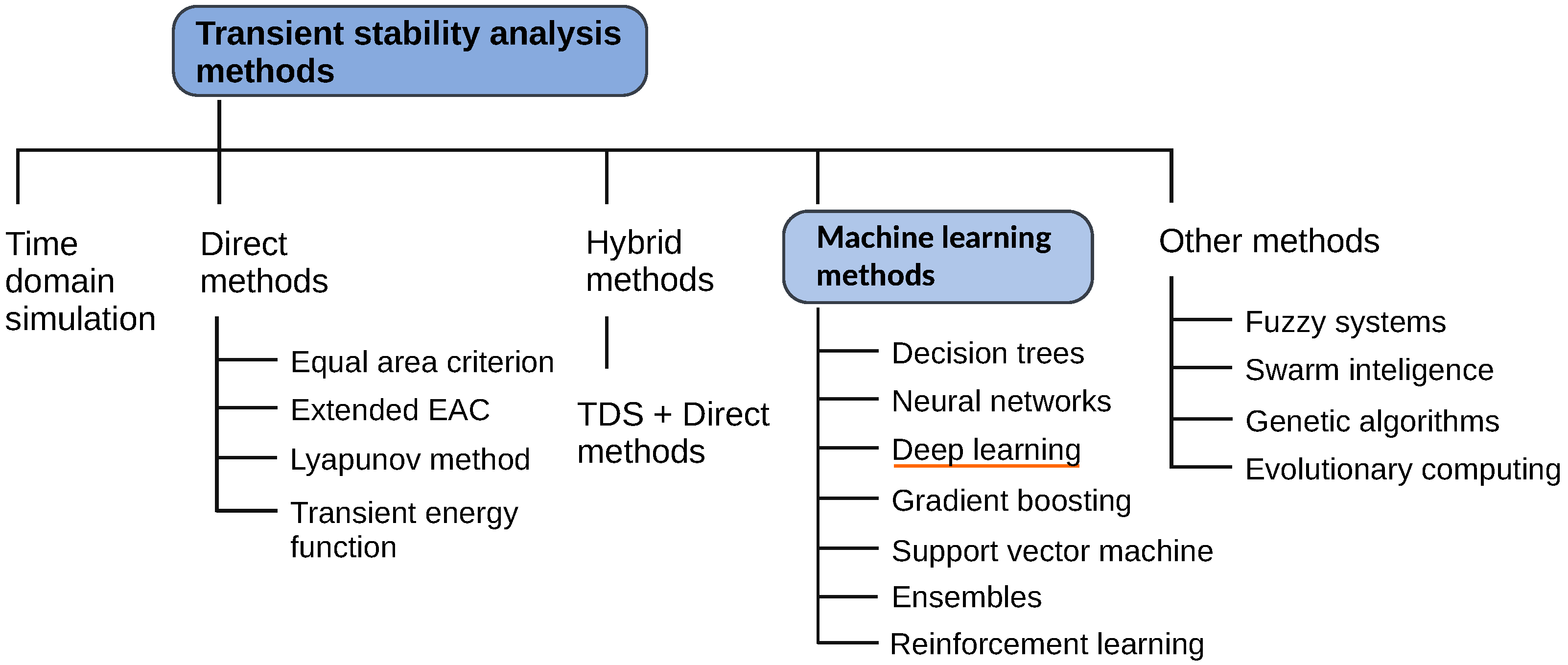
Figure 1 graphically presents a taxonomy of power system transient stability methods [
7]. This taxonomy includes both traditional methods and machine-learning-based methods. However, this review will deal only with different machine learning (ML) methods, as applied to the TSA, which constitute an important part of a broader set of artificial intelligence (AI) applications in modern power systems. The complexity of solving the transient stability of power systems is continually increasing with the availability of various power electronic components, RESs, and AC/DC devices. This makes it increasingly intractable to perform, in a real-time setting, transient energy function or time domain simulations. Hence, it is becoming increasingly common to deal with the transient stability of power systems through the data-oriented paradigm of machine learning.
This review covers several different ML techniques, which can be considered traditional, and then focuses on deep learning (and reinforcement learning) as increasingly important subsets of the wider ML domain. Deep learning, in particular, has recently found a strong foothold in dealing with power system TSA problems. Research for this review was supported by the use of the IEEE Xplore (
https://ieeexplore.ieee.org, accessed on 18 November 2021 ) and Scopus (
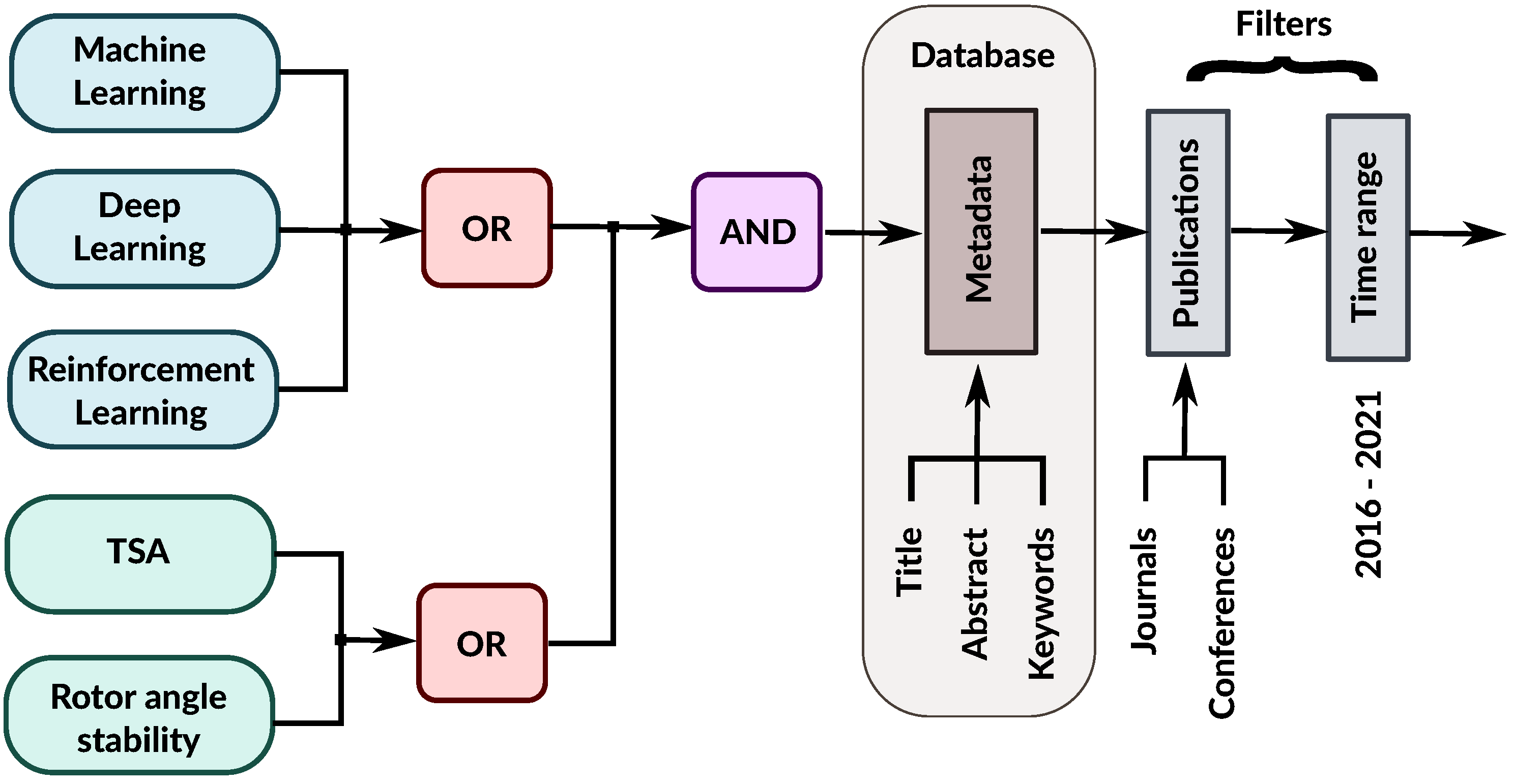
https://www.scopus.com, accessed on 18 November 2021) databases, with the addition of Google Scholar and Microsoft Academic search. Furthermore, the review covers only peer-reviewed research published mostly within the last five years. A search query is designed according to the main criteria that are graphically depicted in
Figure 2. It was successively applied on each of the databases, and the results were pooled together and screened for duplicates. Next, a further selection was undertaken from this pool, by examining the abstracts in more detail. The final selection was hand-picked, using the quality of the research output as the only criterion, to cover the subject area under scrutiny.
The paper is organized in the following manner.
Section 2 introduces a data generation process and describes an overall outline of the data processing pipeline. Both measurement and simulation datasets are covered.
Section 3 depicts a typical AI model life-cycle with all its constituent component parts, from data processing, model building, and training, to model deployment and monitoring. Hyperparameter optimization and estimator performance metrics are also dealt with in this section. Different techniques for building ensembles are briefly described here as well. Next are introduced, also under this section, different machine learning, deep learning, and reinforcement learning models.
Section 4 introduces some of the challenges with existing datasets and models and points to possible future research opportunities. The conclusion is given in
Section 5.
2. Datasets
The introduction of AI in power system transient stability assessment presupposes the existence of the “big data” paradigm, which, generally speaking, emanates from two independent and mutually supportive sources: (a) actual measurements and (b) numerical simulations. Both of these sources of data deal with the power system and have certain advantages and disadvantages. Data coming from measurements have the advantage of representing an actual power system with all the intricacies and possible inconsistencies associated with its contingencies (e.g., generator’s automatic voltage regulator response, characteristic of the turbine governor control, power system stabilizer response, relay protection settings, load shedding schemes, etc.). Measurement data, at the same time, come with the downside of depriving us of the ability of controlling the data generating process itself. On the other side, simulations data offer full control of the data generating process, where we can choose the exact location and types of short-circuit events and other contingencies, and we can experiment with various scenarios. Hence, with simulation data, many aspects of the dataset can be controlled, such as: the diversity of the operational scenarios, and network conditions, the diversity of contingencies, the level of the class imbalance, the level of the data corruption, and others. However, simulation data do not (after all) represent an actual power system, no matter how closely one may model its constituent component parts. Hence, both sources of data bring value to and deserve a proper place in power system TSA and will continue to be used in the future as well.
Datasets are built around the tacit premise that the TSA can be represented, essentially, as a
binary classification problem, where the distinction between stable and unstable cases needs to be clearly established. This is done by introducing a so-called transient stability index (TSI) [
8]. Since the loss of stability in a power system is a low-probability event, the ensuing datasets will be
class imbalanced, which will have important repercussions on the supervised training of machine learning models. Finally, due to possible communication problems between dispersed measurement units in the network, aggregated measured data will inevitably be corrupted with noise and missing values [
9].
2.1. WAMS/PMU Measurement Data
Wide area measurement systems (WAMSs) form an integral part of the modern power system on the high-voltage network levels. With its geographically distributed nature and GPS-time-synchronized measurements, WAMSs can cover wide areas and have certain advantages over traditional measurement systems. The usage of the WAMS is seen as crucial in areas of power system online stability, situational awareness, and security analysis [
10,
11]. WAMS applications include power system condition monitoring, system disturbance management, oscillatory stability monitoring, sub-synchronous oscillation monitoring, power angle stability, and others. Hence, the WAMS provides the foremost solution for monitoring the dynamics of the power system.
The phasor measurement unit (PMU), as an integral WAMS component, provides measurement data for the power system transient stability assessment [
6]. PMU data, at each measurement location in the network, come in the form of time series data (continuous stream of equidistant floating points), sampled multiple times per second, for each of the measured quantities. These can include voltages and currents, active and reactive powers (magnitude and angle for each of the three phases), frequency, and others. Mechanical quantities can also be measured, such as the rotor speeds and angles of generators. All these data are centrally collected, collated, and GPS-time-synchronized. This creates a huge data pool for AI applications.
Papers that utilize actual measurement data are rather scarce, with a few notable exceptions. For example, Zhu et al. in [
12] and Zhu et al. in [
13] both used measurement data from Guangdong Power Grid in South China. Furthermore, measurement data from China Southern Power Grid were used by Tian et al. in [
14] and by several other authors.
2.2. Simulation-Generated Data
Simulation-generated data, as the name implies, are the output of numerical electromechanical transient simulations of the test case power systems. The underlying models of the power system involve complex and very sophisticated representations of its constituent components, where special emphasis is placed on generators with their regulator controls and governor systems. In addition, due to the complexity of individual components, the necessity for a small simulation time step, the large extent of the power system, and the sheer number of constituent components, numerical simulations are very time consuming even on powerful parallel and multiprocessing hardware architectures. MATLAB/Simulink™ is often employed for producing these datasets.
The most thoroughly established power system test case for transient stability assessment is the so-called IEEE New England 39-bus system, which serves as a benchmark and has been employed in numerous papers; see [
6] and the references cited therein for more information. It depicts a part of the power system in the region of New England (USA), apparently as it existed back in the 1970s. This is a rather small power system that features ten synchronous machines, in addition to transmission lines, three-phase transformers, and loads [
15]. One of the generators serves as a surrogate of the external power system (i.e., represents an aggregation of a larger number of generators). Each machine includes an excitation system control, automatic voltage regulator (AVR), power system stabilizer (PSS), and turbine governor control. A single-mass tandem compound steam prime mover, with a speed regulator, steam turbine, and shaft, is used for the steam turbine and governor. A hydraulic turbine with a PID governor system is used for hydro power plants. Each generator can be equipped with multiple PSSs of different types, as well as different types of AVRs and exciters. Loads are represented as simple RLC branches. Transmission lines (TLs) are modeled as three-phase
-section blocks. A high level of familiarity with MATLAB/Simulink is a prerequisite for composing and working with these power system models [
16].
Furthermore, the IEEE 68-bus system (16 machines) and IEEE 145-bus system (50 machines) ought to be mentioned here, as these are somewhat larger test case power systems that also serve as benchmarks [
17]. However, these are far less popular among researchers, with certain notable exceptions, e.g., [
18,
19,
20,
21,
22]. Finally, it can be stated that there are several other test case power systems that have been used for TSA and related analyses, but these are often not fully disclosed and almost always lack certain information.
Even with a small benchmark test case, such as the mentioned New England system, carrying out electromechanical transient simulations with MATLAB/Simulink is very time consuming (seen from the standpoint of CPU time). The sheer number of these time-domain simulations necessary for creating a dataset of even a relatively modest size makes tackling this problem very difficult. Hence, using parallel and multiprocessing capabilities has been explored to reduce the run times needed for creating these datasets. A number of papers have proposed different parallel execution models for reducing the simulation run times [
16,
23]. Furthermore, the authors in [
24] proposed a synthetic synchrophasor generated data as a replacement for real-time PMU measurements. This is still an active area of research.
It is necessary for the datasets coming from actual measurements, as well as simulations, to be openly available to the research community. Furthermore, there is a necessity for more standardized benchmark power system test cases. These should cover a variety of power system sizes and, preferably, should include varying degrees of penetration of renewable energy sources. Most importantly, they should also be openly available to the research community. This is in the interest of the reproducibility of research stemming from the use of these benchmark test cases.
2.3. Features Engineering
Time-domain signals of electrical and mechanical quantities (either measured or simulated) are often post-processed for the extraction of features that are used for the actual training of machine learning models. Broadly speaking, TSA schemes can be divided into pre-fault preventive and post-fault corrective assessments, and the features that will be available from the time-domain signals may depend on the type of assessment. Features can be extracted from many different signals, for example rotor speed, angle and angle deviation, stator voltage, stator d-component and q-component currents, power load angle, generator active and reactive power, bus voltages, etc. Furthermore, features can be engineered from the time-domain and frequency-domain analysis of signals, as well as by combining existing features in different ways [
25]. Namely, many traditional ML models cannot work with raw time series data. Hence, pre-fault and post-fault point values of the time-domain signals are most often used as features for the TSA. This reduces each time series to only two points per signal. Still, even with this reduction of signals to two scalar values, the resulting number of features can be very large for a typical power system. This also means that one often deals with much redundant information and that a large number of features may explode the dimensionality of the features space. This creates difficulty (i.e., the curse of dimensionality) for training ML models.
Choosing the time instants for features extraction depends on the relay protection settings of both generators and transmission lines, where following protection functions will feature prominently: generator under-impedance protection, pole slip protection, frequency protections, distance protection of TLs, and load shedding schemes. There is often a close coordination between the under-impedance protection of the generator and the distance protection of incident TLs, which should be taken into account. At the same time, pole slip protection is specially designed to deal with TSA, but from the point of view of individual generator’s protection. It ought to be emphasized, however, that these different relay protection functions are rarely (if ever) incorporated into the previously mentioned test case power systems.
Dimensionality reduction, features selection, and embedding all provide an effective means of tackling the curse of dimensionality problem [
26]. An
embedding is a relatively low-dimensional space into which high-dimensional vectors can be efficiently translated. Dimensionality reduction can be approached in a supervised or unsupervised manner, using different algorithms, such as: principal components analysis [
27] and its variants, linear discriminant analysis, and truncated singular-value decomposition. It can also be tackled with different types of
autoencoders and by other means. Hang et al. employed principal component analysis [
28]. Several papers proposed different kinds of autoencoders (stacked, denoising, variational), e.g., [
8,
16,
29,
30]. Mi et al. in [
22] proposed a special bootstrap method and the random selection of variables in the training process for tackling the curse of dimensionality. This is still an active area of research, with autoencoders leading the way forward.
3. AI Model Life-Cycle
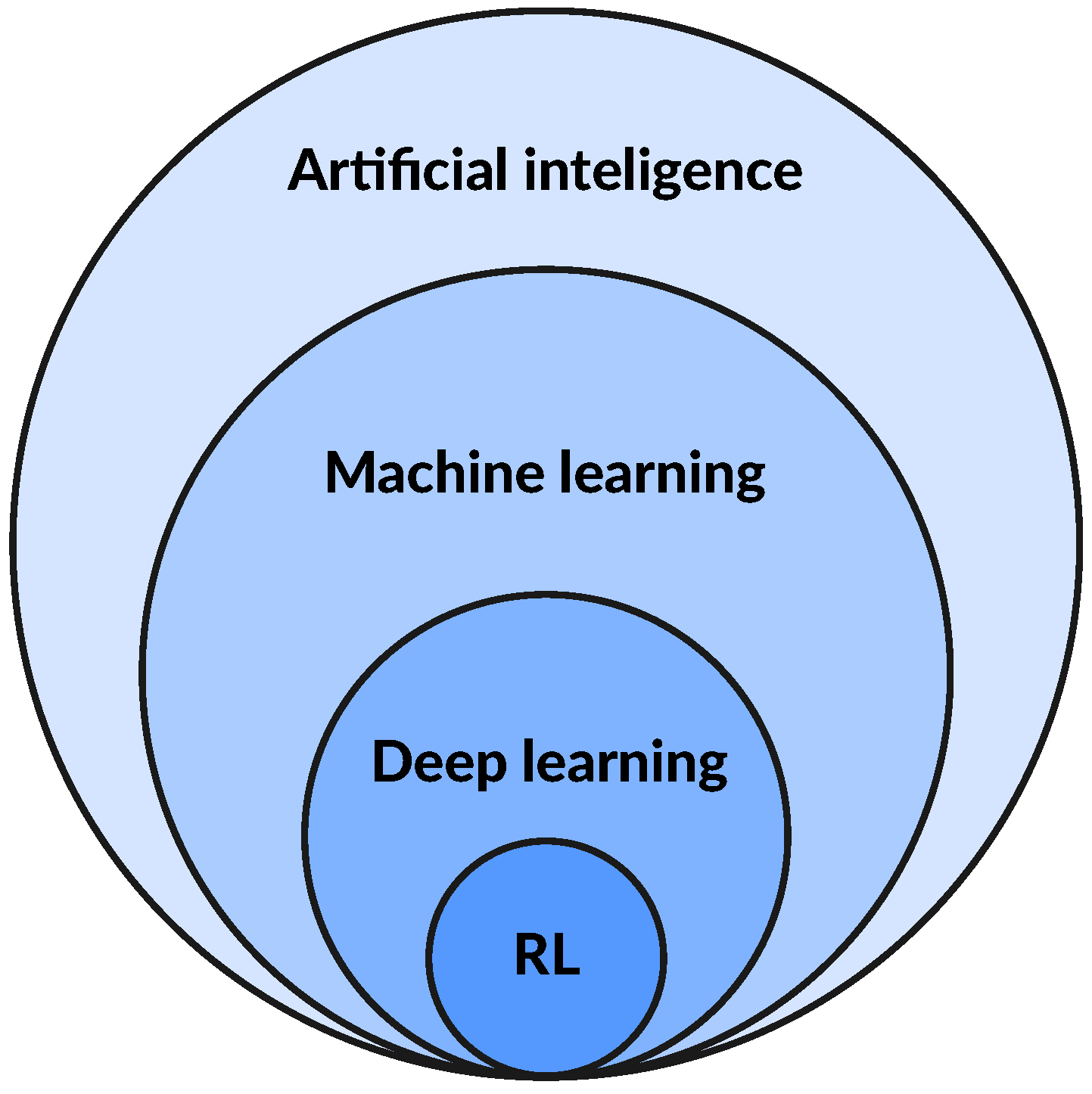
The artificial intelligence landscape is wast and incorporates that of machine learning. Deep learning, in turn, represents only a small, but increasingly important, part of the wider machine learning domain. Finally, reinforcement learning (RL) is a special subset of deep learning, having a unique approach to training models. The situation can be graphically represented by
Figure 3. This review is mainly concerned with machine learning and deep learning subsets, as integral parts of the wider AI landscape, when applied to the power system TSA. Models for TSA are binary classifiers, which learn from data using an offline training, online application paradigm.
Generally speaking, all AI models share a typical life-cycle that usually consists of the following five components: (1) data preparation, (2) model building, (3) model training, (4) model deployment, and (5) model management.
Figure 4 graphically presents the typical AI model life-cycle.
The first phase consists of data preparation, which in general may include several steps, such as data cleaning (e.g., dealing with missing values, noise, outliers, etc.), labeling, statistical processing (e.g., normalization, scaling, etc.), transformations (e.g., power, log, etc.), features engineering, encoding, and dimensionality reduction. The features engineering step is mostly related to traditional ML techniques and it represents a creative component where the majority of the development time is spent. Manual labeling of cases by experts can be costly and time consuming. This first phase also includes splitting data into training, validation, and test sets. Different types of datasets demand specific and appropriate splitting strategies to ensure, for example, properly balanced representations of different classes or satisfying other specific demands. This phase can also incorporate features selection or dimensionality reduction processes. All these steps form the so-called data processing pipeline, which can, sometimes, be more complex than the actual ML model itself.
Next comes the model building phase, closely followed by the model training, where different models can be tried and evaluated for their merits and demerits. A crucial part of the model training phase is the hyperparameter optimization process, which can be particularly time consuming (even on GPUs). Different strategies for tuning hyperparameters can be applied (e.g., grid search, pure random search, Bayesian optimization, bandit-based optimization, genetic algorithms, etc.), with consequential outcomes regarding both model quality and training times. The model building and training phases are mutually intertwined and unfold in an iterative manner, often guided by intuition and experience. The training of deep learning models in particular is still more of a “black art” than a science. Once the models have been trained and fine-tuned (using the training and validation datasets for that purpose), the model building and training phase often yields several prospective candidates. The best model is then selected from this pool of candidate models, based on the performances measured on the test dataset. It is important to ensure that performance measures taken from the test set reflect real-world scenarios and costs associated with the use of the model in the production setting.
This final model, which can be an ensemble, is then deployed. This is the next phase of its life-cycle, which is closely related to the model management phase. Model deployment is concerned with, among other things, its hosting and serving of predictions, while model management deals with the monitoring of the model’s performance and detecting possible problems associated with latency, throughput, and drift. Namely, once the model is actually deployed, it kicks-off a new cycle that begins with the model management. Monitoring, as part of the model management process, provides feedback information for further model fine-tuning and possible retraining with newly acquired data. This corrects for eventual statistical bias and data drift. Inferences derived from monitoring the model after deployment inform the second pass of the model life-cycle. This feedback loop drives model enhancements, and the cycle continues.
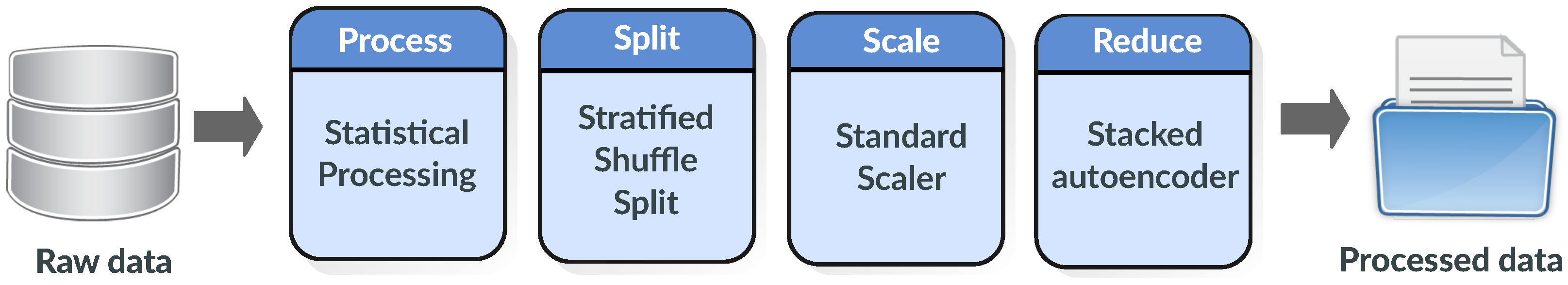
Data processing pipeline example: Power system transient assessment datasets, which have been generated through simulations of benchmark test cases, usually consist of many thousands of time-domain signals of measured (both electrical and mechanical) quantities for the network elements and machines. These data need to be processed by means of a previously discussed pipeline.
Figure 5 graphically presents an example of a data processing pipeline for power system transient assessment data coming from simulations of a benchmark test case [
16]. It features statistical processing of systematic simulations data, followed by the train/test dataset split and data scaling process, and concluded with a dimensionality reduction. This particular pipeline assumes that data already consist of features (vectors/tensors of floating point instances), whatever they may be, which will be fed to an ML model. In other words, features engineering is not part of this pipeline and, if undertaken as an independent step, ought to precede it.
Simulations of benchmark test cases are produced in a systematical manner, by changing the system generation and load levels in certain increments and by systematically distributing the position of short-circuits across the network [
31,
32]. This procedure gives rise to a
systematic dataset, which often does not possess appropriate statistical features. In order to remedy this situation, the pipeline starts by creating a random set from the population of systematically generated cases. This is accomplished by random selection, without replacement, from the population, which yields a statistical distribution with the following properties [
16]: 10% three-phase, 20% double-phase, and 70% single-phase faults. Hence, starting from the population of systematic simulations, this procedure creates a
stochastic dataset that better approximates the power system reality.
In addition, this random selection process preserves the natural
imbalance between the stable and unstable cases, which is an important aspect of the power system TSA problem. An imbalanced dataset (which is heavily skewed in favor of the stable class) necessitates a special splitting strategy that will preserve the class imbalance between the training and test sets. Otherwise, the performance of the machine learning models will be influenced detrimentally by the presence of class imbalance [
21]. Consequently, the next step in the pipeline is a so-called
stratified shuffle split. According to this splitting strategy, first, a total population of training cases is divided into homogeneous subgroups (strata). Then, an appropriate number of instances is randomly sampled (without replacement) from each stratum in such a way so as to obtain a test set that is representative of the overall population. If three separate sets are utilized (training, validation, and test), then the stratified shuffle split strategy needs to be repeated twice; the first pass divides the data into training and validation sets, while the second pass creates a test set from the validation data. The level of class imbalance between all three sets should be preserved after splitting.
The standardization of the dataset, as a next step in the pipeline, is a common requirement for many ML models. Hence, this step standardizes features in the training and test sets. This is accomplished by removing the mean and scaling data to unit variance. Centering and scaling are carried out independently for each feature, by computing the statistics only from the training set samples.
Power system datasets may contain many thousands of features. This high dimensionality of the feature space creates a problem for many traditional ML techniques. Hence, a dimensionality reduction is an important step in the data processing pipeline. A stacked autoencoder can be seen as a very powerful dimensionality reduction technique, which outperforms principal component analysis, and can be made arbitrarily complex. Moreover, it is trained in an unsupervised manner, which means that it can harness huge amounts of unlabeled data. The pipeline can be extended with additional steps, if needed, but the order of the steps is important.
AI cloud infrastructures: The above-described five steps of the AI model life-cycle are often implemented on a purposefully developed cloud infrastructure, which includes purpose-built tools for every step of the ML development, including labeling, data preparation, feature engineering, statistical bias detection, auto-ML, training, tuning, hosting, explainability, monitoring, and workflows. The user can choose between different cloud AI infrastructure providers, such as: Microsoft Azure (
https://azure.microsoft.com/en-us/services/machine-learning/, accessed on 18 November 2021) Machine learning, Amazon AWS SageMaker (
https://aws.amazon.com/sagemaker/, accessed on 18 November 2021), Google Vertex AI (
https://cloud.google.com/vertex-ai, accessed on 18 November 2021), Huawei MindSpore (
https://www.mindspore.cn/en, accessed on 18 November 2021), NVIDIA AI Enterprise (
https://www.nvidia.com/en-us/data-center/products/ai-enterprise-suite/, accessed on 18 November 2021) with VMware vSphere, Paperspace (
https://www.paperspace.com, accessed on 18 November 2021), and others. All these well-known providers offer fully integrated end-to-end cloud solutions for AI development and hosting. They automate many manual tasks and can even completely eliminate software development from the model building (i.e., auto-ML).
3.1. Machine Learning
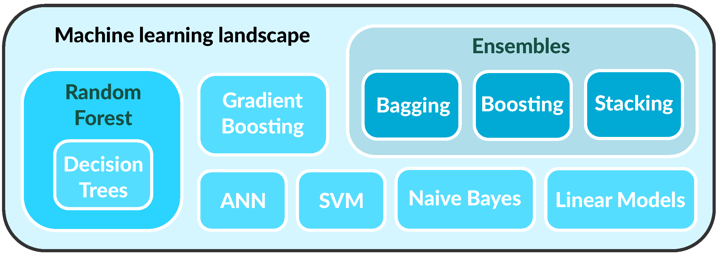
Power system TSA, as a binary classification problem, has been tackled by means of several different traditional ML models. A few prominent ones can be singled out here, such as: support vector machine (SVM), random forest (RF), gradient boosting, and multi-layer perceptron.
Figure 6 graphically presents part of the ML landscape. It can be stated that SVM, including several of its variants, has been very popular among researchers and has shown great promise on benchmark power system test cases. For example, SVM, with or without improvements, was used in [
33,
34,
35,
36,
37]. Several adaptations of the traditional SVM have been proposed as well: core vector machine [
38] and ball vector machine [
39]. Furthermore, a neuro-fuzzy SVM approach was proposed in [
40]. SVM has a small number of hyperparameters, can employ different kernel types, and is fast to train.
The random forest classifier is a meta-learner built from many decision trees, where each tree makes predictions by learning simple decision rules inferred directly from data features. Random forest pools a diverse set of trees and aggregates their predictions by averaging. A twofold source of randomness is introduced to create RF, by growing each tree from a sample drawn with replacement from the training dataset and by splitting each node during the construction of a tree in such a way that the best split is found either from all input features or from its random subset. RF uses two different sources of randomness in order to control overfitting and improve predictive accuracy. Training RF involves a significant number of hyperparameters. Many approaches to power system TSA, involving decision trees or random forests, have been proposed, e.g., [
22,
41,
42,
43,
44,
45].
Several other ML techniques have been applied to the TSA problem as well. For example, Li et al. used extreme gradient boosting machine [
46]. Liu et al. employed kernel regression [
47], while Pannell et al. proposed using the naive Bayes approach [
35].
3.1.1. Hyperparameter Optimization
Hyperparameter (HYP) optimization is a crucial step of the model training process. It can be tackled by using k-fold cross-validation on the training dataset or by utilizing a separate validation set. In either case, the validation split needs to be carried out in a way that preserves the class imbalance. Furthermore, there are many different approaches for HYP optimization, some of which are well suited for situations where there is a large number of parameters of different types, while others are focused on a smaller number of HYPs of a single type. Two well-known general approaches are grid and random search, which are both time consuming and slow to converge. The bandit-based optimization approach (i.e., the Hyperband algorithm) provides a far better alternative and is well suited for tackling a large number of HYPs of different types. When the number of HYPs is relatively small, Bayesian optimization is a good choice [
16]. Genetic algorithms [
6] and evolutionary programming [
48] are still other alternatives appropriate for general use. This is still an active area of research.
Dealing with a class imbalance problem: Datasets on which the ML model is being trained, as was already mentioned, have a class imbalance problem, due to the low probability of power system loss from stability events. This imbalance will influence the classifier in favor of the dominant class. In order to remedy this situation, classifiers use class weighting, which puts more weight on samples from the under-represented class. Weights are adjusted inversely proportionally to the class frequencies in the training data. For that, it is important to preserve the level of class imbalance between the training and test datasets, which is why the stratified shuffle split strategy is needed. It should be mentioned that this is different from sample weighting, which can be used in addition to class weighting.
3.1.2. Ensembles
Ensemble learning is a machine learning paradigm in which multiple models (often called base models) are trained to tackle the same (classification) problem and then combined (by aggregating predictions or with a meta-model) to yield better performance. Models can be combined in different ways, leading to different techniques for creating ensembles (
Figure 6), such as: bagging, boosting, and stacking. Bagging and boosting ensembles use the aggregation of predictions, while stacking ensemble uses a meta-model (i.e., second-level model, which is trained on the outputs from the base models). Because of the two levels, where base models feed data to the meta-model, tracking of the data flow is more complicated for a stacking ensemble. In bagging methods, several instances of the same type of base model are trained independently, often on different bootstrap samples, and then aggregated by “averaging” (e.g., using soft or hard voting). Random forest is a bagging ensemble of decision trees. In boosting methods, several instance of the same base model are trained sequentially such that, at each iteration, the current weak learner adapts to the weaknesses of the previous models in the sequence. In other words, each new base model added to this ensemble boosts the performance of the group taken as a whole. AdaBoost is the most popular boosting ensemble algorithm.
Ensemble learning has been a very popular approach to power system TSA, e.g., see [
17,
28,
40,
46,
49,
50,
51,
52]. Furthermore, several authors have used different tree-based ensembles [
22,
41,
43], or special bagging ensembles [
16,
32,
53]. This is still an active area of research.
3.1.3. Estimator Performance Metrics
Binary classifier performance metrics—when there is a class imbalance present—need careful scrutiny of different error types and their relationship with the associated costs. In power system TSA, a higher cost is generally associated with a missed detection. This is where the confusion matrix gives invaluable support, along with the metrics derived from it (e.g., precision and recall). Notable metrics also include the Matthews coefficient, Jaccard index, and Brier score. Valuable as well is the so-called receiver operating curve (ROC), along with an ROC-AUC score as the area under that curve. Balancing of (unequal) decision costs between false alarms and missed detections can be achieved by using a detection error trade-off (DET) curve plotted in the normal deviation scale. DET curves allow comparing binary classifiers in terms of the false positive rate (i.e., false alarm probability) and false negative rate (i.e., missed detection probability), [
16].
Classifier calibration, as part of the model development process, can be mentioned at this point, which sets the optimal probability threshold level of the classifier. Calibration needs to find a balance point between the precision and recall or between the false alarms and missed detection costs of the classifier. The threshold level that gives this balance, however, depends on the importance of different classifier errors on subsequent decisions and their actual costs. Hence, the calibration process ties together the classifier’s performance with the costs of errors that it makes in production. In other words, the calibration process is concerned with minimizing costs associated with classifier prediction errors.
Machine learning framework example: The Python (
https://www.python.org, accessed on 18 November 2021) programming language is fast becoming a dominant language for data science and artificial intelligence applications. ScikitLearn (
https://www.scikit-learn.org, accessed on 18 November 2021), as an open-source Python library, is probably one of the most prominent frameworks for developing traditional machine learning applications. It features a beautifully designed application programming interface (API), which enables building powerful pipelines, diverse ML models, and complex ensembles. It also streamlines many ML-related tasks, such as: data processing, transforming, scaling, splitting, cross-validating estimators, interchanging different metrics and losses, calibrating and evaluating estimators, model performance visualization, and others.
3.2. Deep Learning
Deep learning (DL) is a popular approach for tackling the power system TSA problem, which still holds great promise and opens future research opportunities [
6,
54]. Deep learning is concerned with the development and training of artificial neural networks (ANNs) with many stacked layers (of different types). However, the training of complex deep neural network (DNN) architectures comes with special problems of proper layer initialization, activation function selection, learning rate scheduling, convergence, vanishing gradients, forgetfulness, dead neurons, and others.
Deep learning’s application to the power system TSA problem does not necessitate a features engineering step, as is necessary with traditional ML models. Namely, these DNNs use
feature learning, which allows a model to both learn the features and use them to perform a classification task. Hence, DNN models can ingest raw time series data, often with only minimal processing, which may include data standardization, using sliding windows, and creating batches. This removes domain knowledge from the model building process, which was needed for engineering features, and lowers the barrier for non-experts’ entry into the field of power system analysis. Having said that, it also needs to be stated that there are situations where significant data pre-processing has been undertaken in order to prepare the raw TSA signals for deep learning [
12,
55]. This is particularly true with DNNs that have been designed for image classification, where time-domain TSA signals need to be converted into 2D images (e.g., by means of frequency histograms, feature space mapping, constructing bitmap representations of spatial–temporal signal correlations, etc.).
The power system TSA problem has been tackled by means of different deep learning architectures, to name here only a few prominent ones: convolutional neural networks (CNN) [
56,
57,
58], recurrent neural networks (RNNs) [
59], networks employing long short-term memory (LSTM) layers [
17,
49,
60,
61,
62,
63,
64] or gated recurrent unit (GRU) layers [
65,
66,
67], generative adversarial networks (GANs) [
9,
68,
69], transfer learning [
70], and autoencoders. These basic architectures can internally vary widely in the number of layers and their stacking order, which allows experimenting with different deep network topologies. CNNs are basically feed-forward ANNs with convolution instead of multiplication as a central operation for updating the layer weights. These networks can also make use of several different layer types (e.g., filters, pooling, dropout, etc.), which are stacked on top of each other for creating deep structures. RNNs, on the other hand, have feedback loops and introduce “memory,” which enables them to learn long time series data patterns. The RNN was a base for developing more advanced layer structures that better learn from long time series data. The GAN approach uses two deep networks that compete in a zero sum game. GANs are very difficult to train. Generally speaking, since TSA data come in the form of multivariate time series, those DNN architectures specially built for long time series analysis have been applied with the most success.
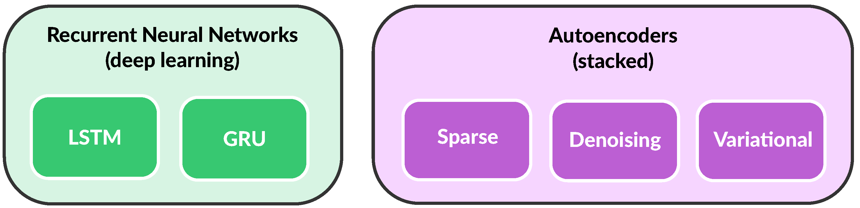
Furthermore, different autoencoder architectures have been proposed for TSA: stacked, denoising, and variational, where the depth and composition of the layer stack of the autoencoder can vary widely [
16,
18,
29,
30,
71]. Autoencoders are prominently applied for dimensionality reduction. They also use unsupervised training, unlike all other deep learning models (except GANs), which use supervised training. This is advantageous, as WAMS data are generally unlabeled.
Figure 7 graphically presents the relationships between RNNs, LSTM, and GRU networks, as well as between different autoencoders.
The application of a feed-forward ANN to the TSA problem, which employs only a stack of dense layers, was given, for example, in [
72,
73]. Yan et al. proposed using a cascaded CNN architecture for fast transient stability assessment [
74]. Architectures featuring hierarchical CNNs [
12] and recurrent graph CNNs [
19] have been proposed. Huang et al. proposed multi-graph attention network in [
20]. Mahato et al. in [
61] introduced a particular Bi-LSTM attention mechanism to the TSA problem, which featured LSTM layers. Wu et al. proposed a deep belief network in [
75]. Xia et al. used an embedding algorithm in combination with deep learning for the transient stability assessment [
76]. Zhou et al. treated the transient stability of a large-scale hybrid AC/DC power grid with the use of deep belief networks [
77]. Ren and Xu in [
9] used GANs, as an unsupervised deep learning technique, to address the missing data problem associated with the PMU observability. As can be seen, some of these neural network architectures make use of graph theory, an attention mechanism, transfer learning, belief networks, as well as several other advanced deep learning features.
Although the application of deep learning to the power system TSA looks very promising, it is also plagued by several unresolved issues. One such issue is the problem of the transferability of DL models across different power systems; see [
12] for more information. There is also the associated issue of the adaptability of trained DL models to constant changes within the power system (development of new RESs, decommissioning of existing power plants, the addition of new transmission lines, network reconfiguration, etc.). Furthermore, the training of deep network architectures with millions of parameters is very time consuming, expensive, and difficult. Clearly, there are still open questions and ample research opportunities in this area.
Deep learning framework example: One of the most prominent open-source deep learning frameworks is TensorFlow 2 (
https://www.tensorflow.org, accessed on 18 November 2021) (TF2), developed and maintained by Google. It features a comprehensive and flexible ecosystem of tools and libraries, including a first-class Python API. TF2 offers multiple levels of abstraction, from the high-level Keras API, down to low-level tensor manipulations and gradient computations. It also features efficient data processing structures (designed to handle extremely large datasets) and can be extended with powerful add-on libraries and models, such as TF Probability. Furthermore, TF Extended enables building full production ML pipelines. A model built with TF2 can be trained on CPUs, GPUs, and even TPUs, without any changes. TF2 is also available inside the previously mentioned AI cloud infrastructures.
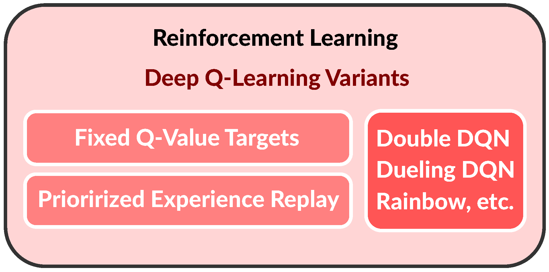
3.3. Reinforcement Learning
Reinforcement learning (RL) is the latest addition to the growing pool of different AI methods for tackling the power system TSA problem. RL is one of three basic machine learning paradigms, alongside supervised learning and unsupervised learning. The typical framing of an RL scenario is one in which the agent takes actions in a certain environment, which is interpreted as a reward and a representation of the state (i.e., observation), which are then fed back to the agent. The purpose of reinforcement learning is for the software
agent to learn an optimal, or nearly-optimal,
policy that maximizes a certain
reward function. The policy is usually a deep neural network, taking observations as inputs and outputting the action, in such a way that balances exploration with exploitation. There are different ways in which this can be achieved.
Figure 8 graphically presents a part of the reinforcement learning landscape, with the emphasis on deep Q-learning (i.e., deep Q-network algorithms (DQNs)).
Reinforcement learning also needs a
simulated environment of the power system in which to train the agents. In other words, the two main components of RL are the environment, which represents the problem to be solved, and the agent, which represents the learning algorithm. It needs to be stated that RL is notoriously difficult, largely because of the training instabilities (oscillations, divergences, freezing) and the huge sensitivity to the choice of hyperparameter values and random seeds. This is a major reason why RL is not as widely adopted as more general deep learning. Reinforcement learning is still a nascent and very active area of research, which has only recently been applied to the power system TSA problem, e.g., see [
78,
79,
80,
81]. Q-learning has been mainly used for this purpose. Clearly, there are ample research opportunities in this area as well.
Reinforcement learning framework example: One of the most advanced and user-friendly RL environments is the Agents (
https://www.tensorflow.org/agents, accessed on 18 November 2021) framework, which is based on the TF2 deep learning ecosystem. The TF-Agents library facilitates designing, implementing, and testing new RL algorithms, by providing well-tested modular components that can be easily modified and extended. This framework may be used to create a simulated environment of the power system for TSA. It already contains many different kinds of agents (including deep Q-learning ones) and provides intuitive ways of designing policies and coding reward functions. Finally, it inherits many of the excellent features of the TF2, on which it stands.
4. Challenges and Future Research Opportunities
The novel paradigm of employing machine and deep learning in power system TSA has proven popular among researchers and has shown great promise on benchmark test cases. However, building the next generation of TSA tools, using data mining and artificial intelligence, is still a work in progress. Namely, stepping from benchmarks into the real-world power systems is often plagued with difficulties emanating from system complexity and unforeseen circumstances. Considering the importance of power systems, there is still ample need for research that corroborates the quality and robustness of this data-driven AI approach to solving the TSA problem. Hence,
Appendix A provides another brief overview of selected research concerning different state-of-the-art AI approaches to power system TSA. This overview presents a snapshot of the current state of affairs, hints at open challenges, and at the same time, points toward future research opportunities.
In the domain of dataset building, several open challenges facing the research community can be identified: (1) open sourcing datasets from power system WAMS measurements, (2) addressing potential security concerns associated with WAMS data [
11], (3) open sourcing existing benchmark test cases, (4) providing a unified and consistent set of benchmark test cases featuring power systems of varying sizes and levels of RES penetration, (5) providing benchmark test cases featuring hybrid AC/DC power grids, and (6) providing standardized simulated environments of power systems for the reinforcement learning. These points deal with standardization of benchmark test cases and bringing them closer to the expected future levels of RES penetration, as well as introducing the hybrid AC/DC power grids [
82,
83]. It also deals with bringing standard simulated environments for RL (i.e., something such as OpenAI Gym (
https://gym.openai.com, accessed on 18 November 2021) for power systems). The hard work of building some of these components is already under way, with the support of the LF Energy (
https://www.lfenergy.org, accessed on 18 November 2021) umbrella organization of open-source power system projects. In the domain of data processing pipelines, challenges include: (1) automatic data labeling, (2) creative features engineering for real-time performance, (3) dealing with the class imbalance problem, (4) dealing with missing data, (5) dealing with data drift, (6) using embedding as a features space reduction, and (7) using autoencoders with unsupervised learning for dimensionality reduction.
In the domain of model building, several issues have been identified with some of the DL-based image classifiers when applied to the power system TSA. In addition, training of deep learning models, in general, is associated with its own challenges: proper layer initialization, learning rate scheduling, convergence, overfitting, vanishing gradients, forgetfulness, dead neurons, long training times, and others. Reinforcement learning models, at the same time, are even far more difficult to train. Furthermore, RL models tend to be “brittle” and may exhibit unexpected behavior.
Tackling these different challenges, at the same time, presents new research opportunities. In the domain of synthetic data generation from benchmark test cases, future research may address the following issues for stress-testing the existing models: (1) introducing different types of noise and measurement errors into datasets, (2) introducing different levels of class imbalances into datasets, (3) introducing different levels of RES penetration into the IEEE New England 39-bus test case, (4) using deep learning for features extraction from time-domain signals, (5) artificial features engineering, (6) experimenting with different stacked autoencoder architectures for unsupervised dimensionality reduction, (7) speeding up numerical simulations of benchmark test cases with parallel processing or by other means, and (8) introducing hybrid AC/DC power grid test cases for transient stability analysis.
In the domain of model building, future research opportunities arise from applying different deep learning models to the power system TSA problem. Employing stacked autoencoders, transfer learning, attention mechanisms, graph neural networks, and other state-of-the-art deep learning architectures is seen as a way forward. Particularly important would be applications of deep learning architectures designed specifically for processing long time series data, image classification, and analyzing graph structures. This is generally seen as a major area of deep learning research, where any novel architecture in this area may be tested on the TSA problem as well. It would also be interesting to see if three-phase signals can be exploited as RGB channels in convolutional layers, with cross-learning between channels/phases. There are research opportunities in devising novel and better ways of converting multivariate TSA signals into images for use with very advanced deep learning image classifiers [
12,
55,
64].
Another major issue with deep learning is a general lack of model interpretability, coupled with the difficulty of understanding the model’s decision-making process. However, there is active research in this area as well. For example, Zhou et al. in [
84] proposed the interpretation of the CNN model decisions for TSA by providing class
activation mapping, which visually reveals regions that are important for discrimination. Activation mapping has been successfully used with deep image classification and can be seen as a way forward for explaining and understanding CNN classifier decisions in TSA applications.
All major deep learning frameworks allow fast model prototyping and training on powerful distributed hardware architectures in the cloud. This levels the playing field for researchers and lowers the barrier for entry. When it comes to model maintenance, TSA is associated with a data
drift phenomenon emanating from steadily increasing RES penetration. Efficiently dealing with data drift is a point of concern for model serving, along with issues of model latency and throughput. Namely, model prediction serving performance (i.e.,
latency) needs to be in real time for maintaining transient stability of power systems following a disturbance [
55]. This limits the computational time available for pipeline processing and may impose certain constraints on its design.
Reinforcement learning has only very recently been applied to the power system TSA problem. The Q-learning algorithm has mainly been explored for that purpose. This provides ample research opportunity for experimenting with different reinforcement learning strategies, with designing efficient policies and reward functions. This area is seen as fruitful and wide open for future research.
Researcher’s resources: It might be of value to mention here several additional resources at disposal to researchers interested in AI applications to power systems. Datasets for the power system TSA applications can be found on Zenodo (
https://www.zenodo.org, accessed on 18 November 2021), which is a premier European general-purpose open data depository, e.g., [
85]. General AI and ML research papers are freely available on arXiv (
https://arxiv.org/archive/cs, accessed on 18 November 2021), where cs.AI and cs.ML would be the subcategories of most interest. Apart from GitHub, the source code that accompanies published research papers can be found from papers with code (
https://paperswithcode.com, accessed on 18 November 2021), which curates ML and AI papers along with their supporting source code repositories. LF AI & Data (
https://lfaidata.foundation/, accessed on 18 November 2021) is a growing ecosystem of open-source projects in support of AI development. Hugging Face (
https://huggingface.co, accessed on 18 November 2021) can be mentioned as a resource that offers the reuse of many different large pre-trained models. Furthermore, some of the popular pre-trained models for transfer learning can be found directly within the TF2. Finally, a PyTorch (
https://pytorch.org, accessed on 18 November 2021) framework, developed by Facebook, can be mentioned here as a capable alternative to TF2. It also offers the Python API and is available inside the previously mentioned AI cloud infrastructures.
5. Conclusions
This paper provided a state-of-the-art of peer-reviewed research, published mostly within the last five years, on the topic of applying machine learning, deep learning, and reinforcement learning to the power system TSA problem. All aspects of the TSA problem were addressed, from data generating processes (both measurements and simulations), data processing pipelines, model building and training, to model deployment and management. A trend is noticeable in the TSA research, which points in the direction of moving from various machine learning techniques to deep learning. Although DL models are far more difficult to train, they do exhibit certain advantages over the traditional ML models. Furthermore, they don not necessitate the features engineering step and can ingest raw time-domain signals (although, sometimes, considerable data processing may be necessary). This automates the process, but removes the expert knowledge from the model building phase. Models are built on the principle of offline training on a large corpus of data and online serving, with a model latency that needs to be in real time. This particular emphasis on model serving in real time needs to be rigorously enforced, considering the fact that predictions need to be utilized as soon as possible (often only milliseconds after the trip of the associated relay protection functions).
The deep learning domain is, generally speaking, still a very active area of research, with several promising avenues: different RNN network architectures (with LSTM or GRU layers), stacked autoencoders, transformers, attention mechanism, transfer learning, and GAN networks, to name a few prominent ones. Deep learning models specifically designed to learn from multivariate long time series data are particularly interesting for applications to the power system TSA problem. Excellent DNN architectures developed for image classification (e.g., Inception, Xception, etc.) offer promising alternatives, provided that multivariate time-domain signals can be appropriately packed into multi-channel 2D images. Exploiting the graph-like structure of the power systems with the use of graph neural networks is another promising research direction. Furthermore, deep learning models that use unlabeled data (such as stacked autoencoders) are very attractive, since data labeling can be time-consuming and necessitates applying humans with domain expert knowledge.
Reinforcement learning, as a special subset of deep learning, is yet another approach that shows early promising signs. However, the training of deep reinforcement learning models is notoriously difficult. The landscape of reinforcement learning is rapidly expanding, which offers ample research opportunities for integrating it with transient stability assessment, particularly in the area of power system control following a disturbance. This is still a relatively nascent, but very promising area of research.
The importance of the electrical power system to society mandates that further convincing results be provided in order to corroborate the stability and robustness of all these various AI approaches. Furthermore, additional and extensive models stress-testing, with different levels of data corruption, is warranted. Potential security issues connected with the wide dissemination of actual WAMS/PMU data need to be addressed as well. This creates space for new research outputs that can fill this gap and increase the overall confidence of the entire community in this new technology, for its safe future deployment across power systems.


