Applying Intelligent Multi-Agents to Reduce False Alarms in Wind Turbine Monitoring Systems

Abstract

This study proposes a method for improving the capability of a data-driven multi-agent system (MAS) to perform condition monitoring and fault detection in industrial processes. To mitigate the false fault-detection alarms, a co-operation strategy among software agents is proposed because it performs better than the individual agents. Few steps transform this method into a valuable procedure for improving diagnostic certainty. First, a failure mode and effects analysis are performed to select physical monitoring signals of the industrial process that allow agents to collaborate via shared signals. Next, several artificial neural network (ANN) models are generated based on the normal behavior operation conditions of various industrial subsystems equipped with monitoring sensors. Thereafter, the agents use the ANN-based expected behavior models to prevent false alarms by continuously monitoring the measurement samples of physical signals that deviate from normal behavior. Finally, this method is applied to a wind turbine. The system and tests use actual data from a wind farm in Spain. The results show that the collaboration among agents facilitates the effective detection of faults and can significantly reduce false alarms, indicating a notable advancement in the industrial maintenance and monitoring strategy.

1. Introduction

Industrial systems can be vulnerable in various aspects, such as components with manufacturing problems, operation under overload, a harsh operating environment, and inappropriate maintenance and human interventions. Some of these vulnerabilities can trigger unscheduled halts for simple maintenance or failures that can damage other systems in the same industrial plant (catastrophic failures), expose people to danger, generate significant economic losses, or even harm the surrounding environment [1,2,3]. In many industrial systems, wind turbines are especially vulnerable because they are electrical power generation units in an open environment. At the top of a tower is a large, enclosed compartment known as the nacelle that shelters essential subsystems and devices, e.g., an electric generator, a mechanical gearbox for rotational speed multiplication, and a hydraulic system [4]. As it is an electromechanical device, it is subject to the vulnerabilities of the electrical power system and the typical wear and tear of mechanical systems. All subsystems of a wind turbine must function properly for long periods to maintain the safety and quality of the supplied electrical energy. To achieve these conditions, maintenance based on continuous monitoring of operating conditions is essential.

Generally, wind turbines and many other industrial systems have several sensors that are already installed at the factory and are part of the supervisory control and data acquisition (SCADA) system. The measurement data of this system are used in the control system of the wind turbine to maximize the generation of electric energy and ensure safe operation under normal and abnormal operating conditions, e.g., high wind speed or short circuits. However, an intelligent system and additional sensors can expand the usage of these data to monitor working and health conditions, and detect numerous fault modes [2,5,6], thus contributing to condition-based maintenance (CBM), increasing the life of the industrial plant, and avoiding catastrophic failures. Many of these strategies and devices are not new and have been developed over the past decades and contributed significantly to increasing the security around the operation, improving the capability of monitoring, and improving the traditional methods of maintenance in critical systems [4,7,8,9].

Among the devices used in the industry for these purposes, soft sensors allow the monitoring of diverse, highly influential physical factors, such as temperature, pressure, force, speed, and vibrations [10]. Some of these physical quantities should remain constant, while others should demonstrate dynamic values and maintain values within a secure margin. When the numeric values of these variables change unexpectedly, it may be indicative of the fact that the system has an incipient defect, a failure in an advanced or catastrophic stage [11,12].

Direct human observation of these variables without appropriate instruments and devices does not permit the exploration of a significant part of the information contained within these fault detection signals. Therefore, many faults can develop rapidly, or even exceedingly slowly, such that the operators and human supervisors cannot extract useful information that necessitates intervention in the systems at an appropriate time to perform preventive or corrective maintenance, thereby decreasing the probability of avoiding catastrophic failures. It was possible to reduce these limitations significantly by incorporating digital computers that allow the processing of these signals through algorithms applying sophisticated mathematical techniques with appropriate precision and speed [12].

Data-driven monitoring methods are easier to implement [13,14,15] but, without the knowledge of the relationships among the diverse subsystems of an industrial plant and the monitored variables, the selection and appropriate use of variables that may reveal some defect or anomaly behavior becomes more difficult. Many studies have considered individualized and isolated approaches to various equipment and industrial subsystems, particularly those that require more time for maintenance, have higher replacement costs, or are difficult to maintain [10,16,17,18]. Therefore, it is possible to lose relevant information from other subsystems and equipment while determining the conditions of operation and health of different components from the same industrial plant.

Principal component analysis (PCA) is a statistical method also based on data. It can detect faults that directly affect the output (monitored physical variable) and generate an alarm; it is ignored when the failures do not interfere with an output variable [13]. Because this method does not distinguish among the process variables related to the monitored output, it generates many false alarms [13]. A more robust technique is the partial least squares (PLS) technique that extracts information related to the output by monitoring another variable, that is, the input. This method still has limitations in failure detection, and it generates a significant residual space.

Although the literature presents various solutions for monitoring and fault detection in industrial plants, there are still numerous open questions that motivate this study, for example, the lack of a systematic methodology to create monitoring and fault detection systems applicable to different types of industrial plants. Likewise, it is necessary to develop new methods to aggregate real measurement signals from different subsystems of the same industrial plant and even combine well-established algorithms to produce new methods and indicators to reduce false alarms.

2. Related Work, Objectives, and Contributions

So far, it is possible to see that data-based monitoring and fault detection methods have great potential to be used in conjunction with multi-agent systems (MAS). A statistical method of monitoring based on data was demonstrated in [19], which showed that an MAS was also suitable for managing and controlling various aspects of microgrids, including market operation, fault location, microgrid protection, and service restoration. Eddy et al. [20] proposed an MAS method for managing distributed generation with price-driven generation in an electric microgrid, including wind turbines. The first example above, in [19], uses computer agents developed on the Java Agents Development Platform (JADE) [21], while the second example in [20] demonstrates the possibility of using the agent development platforms JADE, ZEUS, and VOLTTRON.

These data-driven techniques, in which monitoring models involve several input variables related to an output variable, are challenging to obtain using conventional linear regression techniques. Because of the complexity of many industrial systems, highly nonlinear relationships can exist. To address the difficulties to create monitoring models for systems with multiple nonlinear physical variables, it is possible to develop data-driven models based on normal behavior, which can be achieved through various mathematical and computational techniques, for example, through ANNs [22,23], signal trend analysis in industrial plants [16], and multivariate statistical techniques [24].

Among these diverse techniques, the nonlinear auto-regressive exogenous artificial neural network (NARX ANN) was used in [22], where the output of the anterior instant (t − 1) of ANN was utilized for incipient fault detection on the bearings of the gearbox of a wind turbine. Therefore, they used the output of the ANN to calculate the Mahalanobis distance, which effectively determines the presence of anomalies. In [23], an ANN model can detect a set of physical variable values of a wind turbine that are out of normal operation. Next, these points are used to generate self-organizing maps (clusters), whose patterns are modeled through a discrete-time Markov chain for mid-term analysis of the operation.

The method presented in [16] is based on a memory matrix with normal behavior data. Each column of the matrix represents the state of the monitored variables of the industrial process or device at the same instant. However, to generate a matrix with only new states, the Euclidean distance between all the vectors of states that already constitute a part of the matrix and a new candidate state is calculated, and the distance should be larger than a defined threshold. With a low interpolation capability in the addition of new states, this methodology does not outperform the neural network method. In [24], a method for the prognosis of a wind turbine gearbox is presented; however, in this case, it directly uses the Mahalanobis distance to determine multivariate outliers in the low-frequency SCADA data without the need to label the data manually.

2.1. Objectives

This study proposes a method for monitoring the operational conditions and detecting faults in industrial plants through models based on normal behavior using ANNs, while utilizing the interaction of models through intelligent agents to increase the monitoring performance. Therefore, it differs from the methods based on normal behavior presented in [16,22,23,24], where directly measured data are used in the ANNs and establish dynamic fault detection ranges according to the operating conditions of each subsystem of the industrial plant. Because it is a data-driven method, the SCADA measurements of a real wind turbine are utilized to develop the models, agents, and tests. The models are strategically generated based on the results of failure mode and effects analysis (FMEA) [25]. For a more comprehensive approach, applying the FMEA facilitates selecting variables and establishing pertinent relations among diverse equipment and subsystems from the same industrial plant for the construction of valid models rather than using an approach on specific equipment of an industrial plant, as presented in [16,22,24,26,27,28]. Thus, the proposed method leverages information from multiple subsystems to improve the diagnostic capability and uses FMEA to help design this integration. This analysis suggests that these measurements should be monitored to prevent or alert for the presence of possible failures. In the proposed method, the agents co-operate more explicitly, in contrast to those proposed in [19,20]. This study also aims to create a general or global indicator of the operating conditions and health of industrial plants but without isolating the subsystems that cause sudden changes in operating conditions, as is carried out in [6].

2.2. Contributions

A set of agents is designed and implemented to perform this function; their interaction and co-operation contribute to reducing false alarms. Thus, it is a more comprehensive approach than the existing models that use simple monitoring of an output variable or monitoring an output variable through an input variable. The major contributions of the proposed method are as follows:

• Establishment of a methodology that can be used to develop a system for monitoring industrial systems;
• Utilization of information from various subsystems of an industrial plant to improve the ability to monitor and detect faults;
• Improvement of the certainty of diagnosis of working conditions of industrial systems through reduction in false alarms by combining MASs and behavioral models of normal behavior generated using ANNs;
• Establishment of a single indicator for the operating conditions of all the subsystems of a plant. This novel monitoring system based on plant operating conditions, with reduced false alarms, based on neural models as multi-agents, presents considerable potential for assistance in the diagnosis and maintenance activities of industrial systems.

The remainder of this paper is organized as follows. Section 3 presents the proposed method for condition monitoring of industrial processes. Section 4 describes the application of the technique for a wind turbine, and Section 5 presents the results and related discussion. Finally, the conclusions are presented in Section 6.

3. Method for Condition Monitoring of Industrial Processes

This section summarizes the crucial steps of the proposed method for the development of a platform for monitoring the operating conditions of industrial processes, as shown in Figure 1.

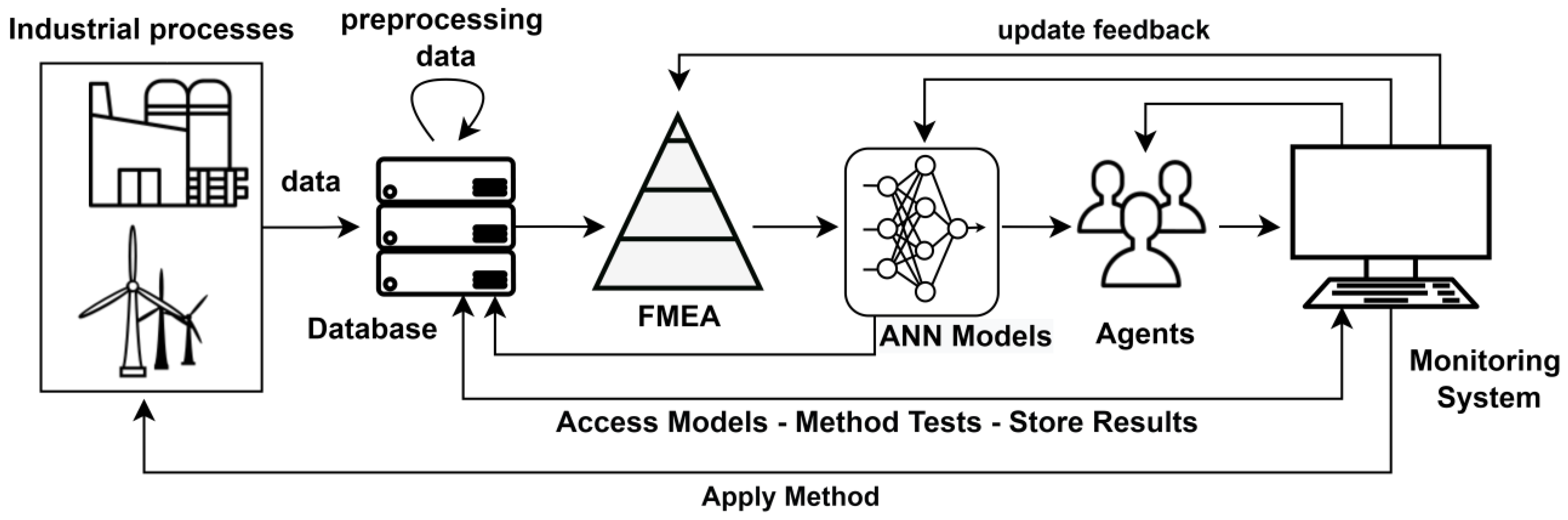
Figure 1 presents the different steps of the novel method proposed for the monitoring and early detection of anomalies in the operating conditions of equipment in industrial processes:

• Industrial processes: depending on the industrial plant, it is necessary to use sensors to monitor the mechanical and electric variables. If feasible, sensors may be installed during the manufacture of equipment, or a set of appropriate sensors may be installed with conditioning and acquisition signal interfaces in various systems and devices in the industrial plant to be monitored.
• Database: it is necessary to store data conveniently for a sufficiently long time for developing and testing data-driven monitoring models.
• FMEA: FMEA is employed to select the most appropriate signals for industrial processes to develop mathematical or computer models for monitoring and fault detection.
• ANN models: ANN models are developed for anomaly detection using signals determined via FMEA.
• Agents: it is necessary to design intelligent agents that can temporarily store and execute the ANN models developed in the previous step. To avoid developing intelligent computational agents with good characteristics from scratch, it is possible to use flexible platforms for creating intelligent agents, such as JADE.
• Monitoring System: to develop and test the monitoring system, the agents must load the monitoring and fault-detection models stored in the database. The system must also attempt to use the old data stored in the database and new data sent by the industrial plant on the models and store the results. The system should also generate a list of anomalous behaviors of the monitored signals and trigger alarms.

As shown in the diagram in Figure 1, connections among the blocks refer to the updates based on the test results. According to each block output, it may be necessary to perform the FMEA again and update the ANNs and agents. If the FMEA is satisfactory, it may be necessary to update only the generated ANN models and intelligent agents.

In the development phase of the monitoring system, it is possible to use offline data already stored in the database and update the models. If there are sufficient conditions for compatibility, it is possible to apply all the steps used to develop this condition monitoring platform to other similar plants.

This method of monitoring the operating conditions was applied to a wind turbine, as presented in Section 3.

The following subsections describe each step of the method described in Figure 1.

3.1. Preprocessing of Digital Data

The data measured in industrial plants are often not suitable for the development of good computational and mathematical models for monitoring systems, fault detection, and diagnosis; therefore, it is essential to preprocess these signals correctly [29]. Thus, preprocessing is one of the most important and time-consuming steps in the development of computational intelligence models [30]. Even after the computational models are created, the automatic analysis of the input data of these models that occur in a continuous flow is also very important to provide adequate outputs [30]. Thus, in the data preparation step, it may be necessary to perform several steps, such as data cleaning, data transformation, data integration, data normalization, missing data imputation, noise identification, and data reduction [31].

Several conditions can produce errors in the measurements of the sensors, analog-to-digital conversion, local storage, or the transmission of digital data if the storage is remote. These conditions can be related to severe environments where electromagnetic interferences, mechanical vibrations, excess humidity, and dust may occur in various devices, such as sensors, transducers, signal conditioners, data storage elements, and apparatus transmitting analog and digital signals [32].

There can be various anomalies, even in digital data. Among the most common problems that can occur are errors in the scale due to signal conditioning, outliers, samples not acquired at a single point or in sequence throughout the time series, and synchronization error of the various time series of the different signals measured and stored in the databases [29]. To deal with anomalies in digital data, numerous algorithms have been developed, for example, to identify outliers. One can calculate the local outlier factor (LOF), and thus determine whether measurements have values that are too far from the neighborhood [32]. Similarly, statistical methods based on the moving average can also be used to identify outliers. Fortunately, many of these algorithms can be found in ready-made functions in popular computer programs, such as MATLAB, WEKA, Python, and Scikit-Learn. MATLAB, for example, features the functions isoutlier() and isnan(); the first function is able to evaluate a set of samples and determine which are outliers, according to the configuration parameters, and the second whether a digital datum is or is not a number. However, in the implementation phase of the monitoring system, it is necessary to develop specific preprocessing functions in the supervisory software itself in its respective programing language, or it must support the use of libraries created in programs to develop computer models.

3.2. FMEA Applied for Variable Selection in Industrial Processes

FMEA is a well-known procedure used to evaluate the risks, impacts, and costs of failures in industrial systems, their diverse subsystems, and equipment [25].

In this study, the FMEA technique is used to establish a monitoring and maintenance strategy for industrial systems to maintain appropriate working to the extent possible. It attempts to establish a hierarchy of the influence of failures and consequences on the various subsystems, components, or parts, so it also supplies the effective variables to be analyzed. An increase in ambient temperature, for example, can affect all the subsystems in a plant, but the temperature increase of only one device rarely affects the entire industrial plant. Thus, monitoring through sensors at the component or part level becomes increasingly important for identifying and isolating the failure, that is, locating the device in which a particular fault has occurred [25].

3.3. ANNs for Condition Monitoring Models

This step aims to generate optimized neural network models using the signals selected in the FMEA. Industrial processes present numerous physical states or dynamic variables that can be monitored using sensors. However, it can also have a few internal states that cannot be observed directly; other states require costly sensors; therefore, their use in many industrial plants with commercial objectives is not economically viable.

Some of these physical states can reconstruct mathematical states through ANN models, thus establishing an approach for verifying whether the behavior of the monitored state is following the variables of the input model [13]. It is necessary to perform numerous tests using various parameters to obtain an optimal ANN model, such as:

• Division of the data from training into three groups (training, validation, and testing);
• Determination of the training algorithm;
• Selection of criteria for termination of training phase;
• Definition of the inputs of the models;
• Specification of the number of layers of ANN;
• Specification of the number of neurons in the layers of ANN.

The division of data into three different subsets aims to create models that perform well on the data on which they have not been trained (generalization). The first subset serves the ANN training; the second should be reserved for performing convergence validation and applying the training stopping criterion to avoid underfitting and overfitting the reconstructed state functions; and the third subset is used for testing [33]. Thus, a more significant part of the signal sample is used to train the ANNs; smaller and equal portions of the samples are reserved for validation and testing.

The Levenberg–Marquardt algorithm can train the ANNs because it has an appropriate training speed, faster convergence, and excellent performance in classification models, numeric regression, prediction, and pattern recognition [34,35].

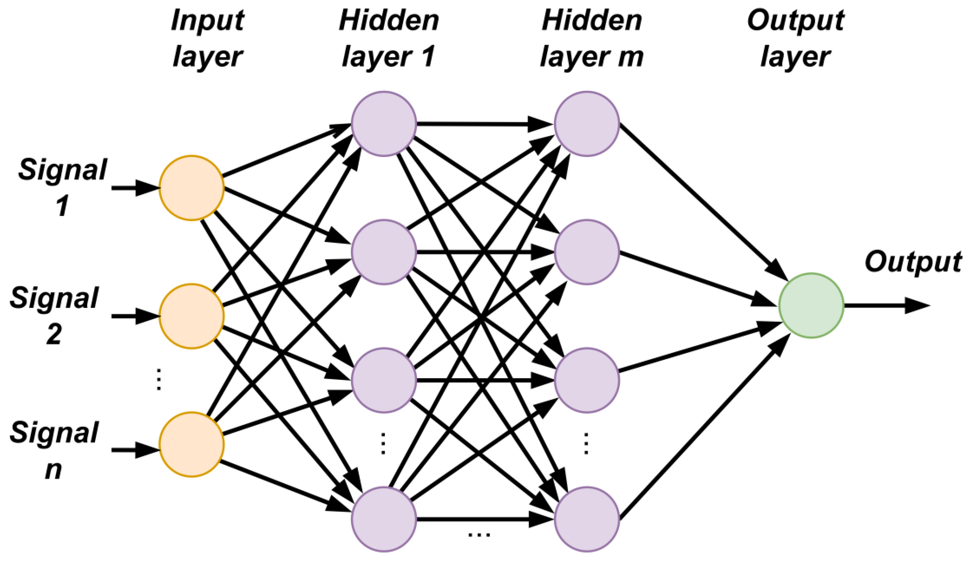
Figure 2 shows the simplified generic topology of a multilayered neural network that varies the number of inputs, hidden layers, and neurons in each layer [33].

Because each topology has a different performance, it is necessary to verify the performance of a group consistent with topologies to obtain an optimized model. The topologies can be chosen randomly, heuristically, or several parameters can be progressively varied to assess the performance of several different topologies.

In the method used in this study, the topology of the ANN models is varied as a function of the number of layers and the number of neurons. Then, the mean square error (MSE) is computed with the testing dataset for each topology and applied to assess its performance (see Appendix A). Due to the random initialization of the synaptic weights, it is necessary to repeat the training of each topology for various initializations because it can converge to significantly better or worse values after the training phase.

According to Figure 2, it is convenient to automatically distribute the number of neurons of the layers to test the different topologies. For networks with only one hidden layer, all the neurons are in this layer but, for networks with two hidden layers, it is necessary to divide the number of neurons between the two layers. In this manner, to obtain an integer number increment of the number of neurons, the following equation can be used:

$$\lceil \frac{n}{2}\rceil :\lceil \frac{n-1}{2}\rceil$$

(1)

The function ⌈ ⌉ represents the rounding of the entire number above (ceil(.)), and n represents the total number of hidden neurons in the network distributed among the hidden layers. The colon sign separates the number of neurons in each hidden layer.

Similar to ANNs with two hidden layers, dividing the hidden neurons into three layers is also necessary. Thus, to obtain an integer unit increment of the number of neurons for each layer, the following equation can be used:

$$\lceil \frac{n-1}{3}\rceil :\lceil \frac{n}{3}\rceil :\lceil \frac{n-2}{3}\rceil$$

(2)

One of the problems to be aware of when training ANNs is overfitting due to the following reasons [36,37]:

• Difficulty in obtaining the ideal neural network topology;
• Existence of samples in the input variables with entirely different values from the contiguous samples or from the entire time series (outliers);
• Complex training algorithms hindering convergence [36];
• Training the ANNs with an exceedingly large or small amount of data.

3.4. False Alarm Detection Strategy

The purpose of this subsection is to demonstrate the use of optimized models to detect false alarms. It is possible to detect false alarms using the estimated values of the expected behavior of the different parts of an industrial system. First, it is necessary to obtain the expected values of some measurements of a plant signal. The nth estimated value of the signal time series can be obtained using the following equation:

$$\widehat{S}\left(n\right)=M_S\left(S_1\left(n\right),S_2\left(n\right),\dots ,S_k\left(n\right)\right)$$

(3)

where $\widehat{S}\left(n\right)$ is the estimated value for the signal $S\left(n\right)$ signal, for the sample $n$ of the temporal series, and $M_S$ represents the ANN model of the agent $S$ that monitors the physical signal of the industrial plant and is named with the same letter. The model $M_S$ has $k$ signal inputs $S_1$, $S_2$,…, $S_k$ and may represent signals of an industrial process, such as pressure, temperature, and wind speed. Although the signal $S$ is generally different from its model input signals, it can also be of the same type as well. The signal estimated using the input signals and the input signals themselves are chosen after the FMEA analysis. After obtaining the signal estimated for the nth sample, it is necessary to calculate the estimation error $\epsilon \left(n\right)$ of the signal that is given by Equation (4):

$$\epsilon \left(n\right)=S\left(n\right)-\widehat{S}\left(n\right).$$

(4)

This error is used to estimate a maximum value for the error that determines whether an estimated behavior of a variable is outside the range of values expected for normal behavior for the normal operating condition of a subsystem of an industrial plant. Thus, the error calculation is also performed using all the samples used in the training period of each ANN model separately. The maximum error value or threshold covers 95.44% (approximately two standard deviations, $2\sigma$) of all the calculated errors in a Gaussian distribution and is used for the new samples that are different from the training data; this method is similar to that proposed in [38]. Because these thresholds of each monitored signal are calculated directly from the data of normal operation of the diverse subsystems of an industrial plant, an expert does not have to determine these values initially. Using normal values or values within the normal behavior range of various signals from an industrial plant to train models is an essential characteristic of this study [23,24]. For systems where it is necessary to use stricter constraints on normal behavior, even smaller error margins can be used.

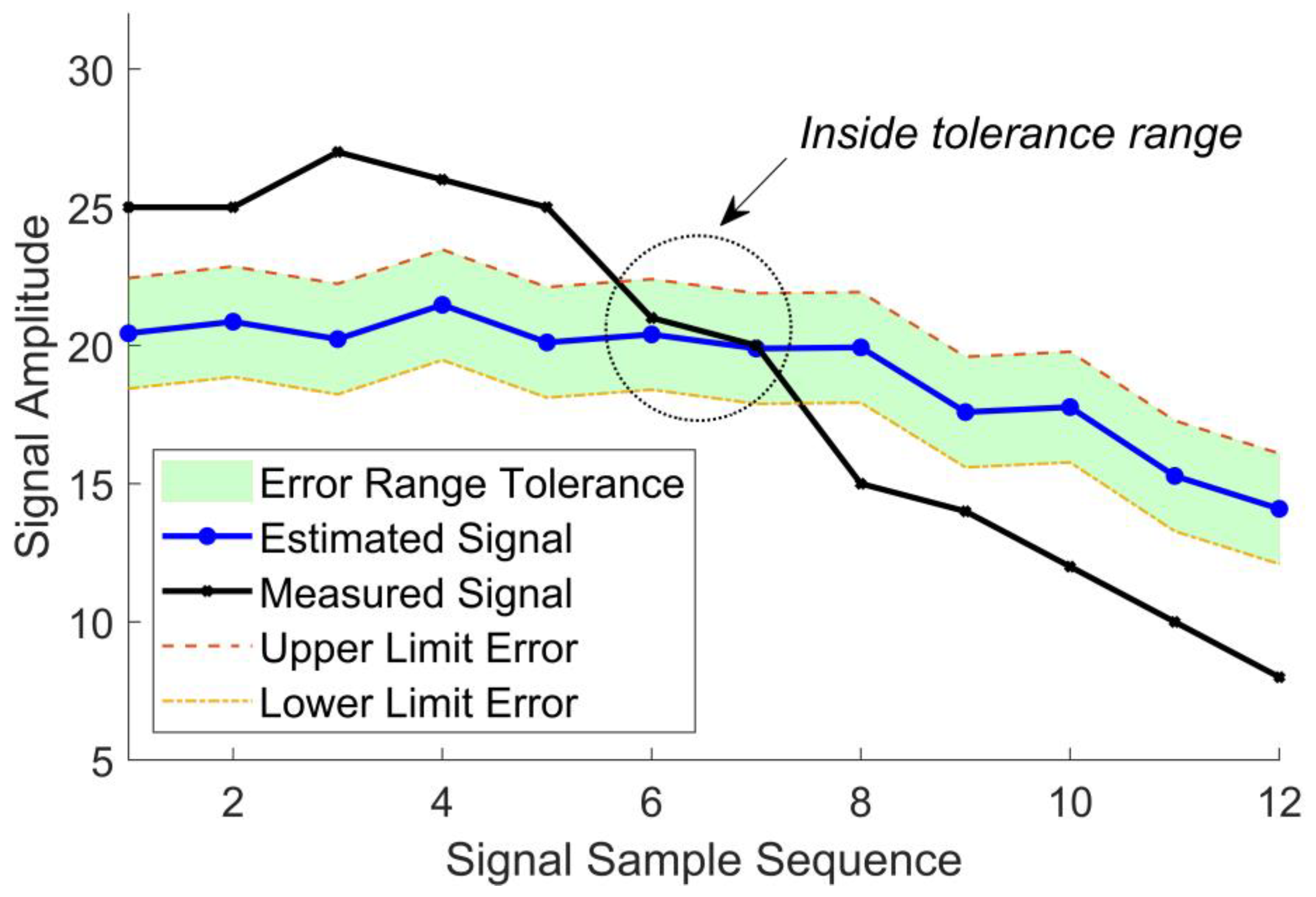
If the absolute value of the error is greater than the threshold calculated for each ANN model with normal behavior, an alarm should be computed according to Equation (4). Figure 3 shows a region shaded in green. The dashed line (upper error limit) and dotted line (lower error limit) limit the green area. The upper $S_{max}\left(n\right)$ and lower $S_{min}\left(n\right)$ limits of the measured signal $S$ for the $n$ samples are given by the following inequations, respectively, such that it is not considered as an alarm.

$$S_{max}\left(n\right)\le \widehat{S}\left(n\right)+{\epsilon }_{maxS},$$

(5)

$$S_{min}\left(n\right)\ge \widehat{S}\left(n\right)-{\epsilon }_{maxS},$$

(6)

where ${\epsilon }_{maxS}$ is the value that covers 95.44% of all the calculated errors in the training step for the normal behavior of signal $S$ of an industrial plant.

For industrial plants and their subsystems where the operating conditions allow, it is also important to generate different alarms of medium duration, such as generating alarms when an uninterrupted sequence of alarms occurs. This situation implies that incipient or persistent catastrophic failures may occur.

3.5. MAS for False Alarm Detection

The purpose of this subsection is to demonstrate the strategy used to detect false alarms using MASs. The agents should form groups, known as fundamental elements, that can play a co-operative role, thereby performing better on many computational tasks than a single agent [20,39].

Many industrial systems have a distributed nature with a large amount of equipment, and an MAS is an appropriate tool to generate a platform for monitoring and performing fault detection. Using a multi-agent platform affords more flexibility for various purposes: the expansion of new intelligent models, distributed processing for over one computational unit, and robustness of agents in case of faults that ensure continual operation of agents not affected by the faults inside a fundamental unit [40,41].

In this study, the agents evaluate the operating conditions of a subsystem or equipment of an industrial plant and perform the function of rejecting false alarms of other subsystems by sharing signals in the other monitoring models.

The previous subsection showed that the alarms arise when an error in the estimation of the measured signal is greater than a threshold; thus, in this study, the errors are calculated relative to the values expected by the ANN models. Frequently, these errors, the difference between the estimated signal of the ANN model of normal behavior and the measured value of the signal, can be outside the expected confidence range, implying a deviation from the expected normal behavior. The confidence ranges are based on the error of the model observed during its training plus/minus twice the standard deviation of the mean error found. However, these alarms do not always mean that the signal is outside the expected range. Because the models also receive at their input measured signals that are also subject to incorrect measurements (defective sensors) or values affected by noise that can cause errors in the estimations, these cases are known as false alarms. To deal with these cases, the development of a method for detecting false alarms is also very important.

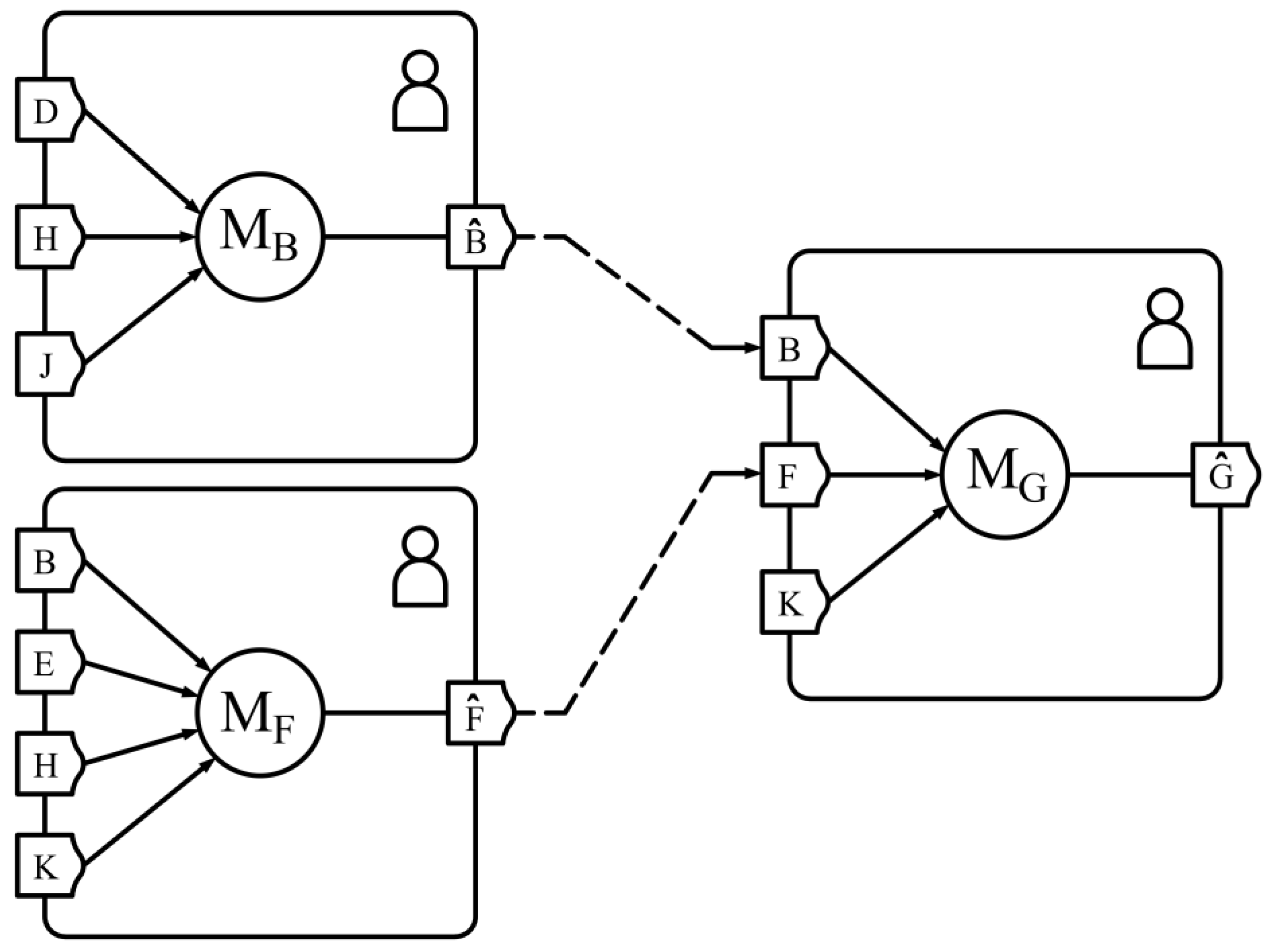
Therefore, a novel method based on agents is proposed to reduce the possibility of false alarms. As shown in Figure 4, the agents interact with each other, where the models and interconnections of B, F, and G enable the agents to analyze the estimation error of normal behavior [41,42].

Figure 4 shows the agent with model M_G that performs alarm rejection based on the analysis of the outputs of the predecessor agents with models M_B or M_F. The analysis is based on the sensitivity of the model M_G to variations in the input signals. The following calculations should be performed to evaluate the sensitivity of the model $M_G$ for the outputs of the models $M_B$ and $M_F$:

$${\epsilon }_1=G-M_G\left(B, F, K\right),$$

(7)

$${\epsilon }_2=G-M_G\left(\widehat{B}, F, K\right),$$

(8)

$${\epsilon }_3=G-M_G\left(B, \widehat{F}, K\right),$$

(9)

$${\epsilon }_4=G-M_G\left(\widehat{B}, \widehat{F}, K\right).$$

(10)

M_G is an ANN model trained for the normal behavior of a signal named G of an industrial plant. The signals B, F, and K are inputs of the M_G model and are physical signals of the same industrial plant, monitored equipment, or environment, for example, environmental temperature. Environmental variables rarely require agents to monitor their state unless the industrial plant can influence these physical quantities because of an operating regime or any other condition. However, their values can be applied to the inputs of the ANN models.

For detecting false alarms, three conditions that define the magnitude of change in its estimates based on the changes in the inputs are:

• Either $M_B$ or $M_F$ in Figure 4 must present an estimation error that exceeds the error threshold (the analysis is conducted independently and sequentially); thus, the a priori presumed alarm should be analyzed by the model $M_G$;
• The $M_G$ model must present a small error when it receives all the measured signals as its inputs, thereby indicating that it can process the agent outputs $\widehat{B}$ and $\widehat{F}$ simultaneously;
• The estimated values for the normal behavior of the models $M_B$ and $M_F$ are supplied as the input to the model $M_G$. Accordingly, four errors are calculated using the estimated values of models $M_B$ and $M_F$, as shown in Equations (7)–(10). Each error is calculated independently and sequentially. If the ${\epsilon }_2$ is larger than the established limit of $M_G$, this implies that the estimation provided by the predecessor $M_B$ model is incorrect. Thus, it is interpreted as a false alarm of $M_B$. If the ${\epsilon }_3$ is larger than the established limit of $M_G$, this implies that the estimation provided by the predecessor $M_F$ model is incorrect. Thus, it is interpreted as a false alarm of $M_F$.

The analysis of ${\epsilon }_1$ and ${\epsilon }_2$ verifies whether model $M_B$ generates a false alarm. The analysis of ${\epsilon }_4$ does not contribute to the analysis of the origin of the error because it considers the estimations of the B and F signals as inputs; thus, the cause of the error is unclear because it may have been caused by the estimated value of B or F.

The analysis of the errors ${\epsilon }_1$ and ${\epsilon }_3$ allows us to verify if the M_F model generates a false alarm, and the three conditions announced above are mathematically detailed below:

• For condition i: $\left|\widehat{F}\right|>E_{maxF}$: an a priori presumed alarm occurred in the M_F model;
• For condition ii: $\left|{\epsilon }_1\right|<0.2·{\epsilon }_{maxG}$ (20% of the maximum error limit of the G signal estimate is empirically assumed to be a small error);
• For condition iii: $\left|{\epsilon }_3\right|>{\epsilon }_{maxG}$.

$\widehat{F}$ is the estimated value of signal $F$; ${\epsilon }_{maxF}$ and ${\epsilon }_{maxG}$ are the maximum limits of the defined errors for the signals $F$ and $G$, respectively. Similar conditions should be considered when analyzing the estimation of signal B.

It is considered a false alarm when at least one of the agents in a group of agents classifies it as a false alarm. This final analysis, which considers the responses of all the agents, is performed using a synchronizing agent.

3.6. JADE Agent Architecture

The previous subsection showed how agents process signals from an industrial plant through ANN models trained for normal behavior. The interaction of the agents through the neural network models is aimed at reducing false alarms.

This subsection describes how the features of the agents can be used to generate monitoring agents, explains the various interfaces with the program operator and the methods employed to ensure co-operation among the agents, and the messages exchanged among the multiple agents.

An important aspect that must be considered is the use of a standard communication language among agents. A well-known communication standard among intelligent agents is the Foundation for Physically Intelligent Agents—Agent Communication Language (FIPA-ACL) [22]. It contributes to the development of flexible systems that can communicate, even with different systems and platforms. Among the agent development platforms presented in [19] (JADE, ZEUS, and VOLTTRON), the JADE platform has been chosen because it is the only platform that is simultaneously compatible with the FIPA-ACL standard, based on JAVA, which is a free and open-source software platform and still has active support.

An agent must act or react whenever necessary to send or receive data, apply the intelligent models to a new sample of the signals, graphically present the processing results to the operator, and store the results. All the agents must have logic and programing structures called behaviors to perform these tasks in a co-ordinated manner when data and new samples of plant signals become available. These structures can be obtained by programing and using the JADE platform to generate computational agents [21].

One of the most critical behaviors, known as cyclic behavior (CyclicBehaviour, a JADE class in Java), is used in all the agents, such that it is possible to monitor new messages from the other agents. The synchronization agent is based on clock behavior (TickerBahaviour, a JADE class in Java) to verify the availability of new samples of measurement and send them to the intelligent agents.

A library provided by JADE also has a basic structure that allows communication among agents on the same computer or other computers over the Internet. However, the programmer must design the block code to interpret the messages, load the ANN models onto the agents, and define the appropriate time to transmit the messages under the necessary conditions.

Agents must be able to load the normal behavior models of ANNs from the database and run them. The JADE platform allows the development of graphical interfaces as a traditional supervisory program for each agent, such that the maintenance team operators can easily interact with the monitoring system.

3.7. Programs for Implementation of the Suggested Strategy

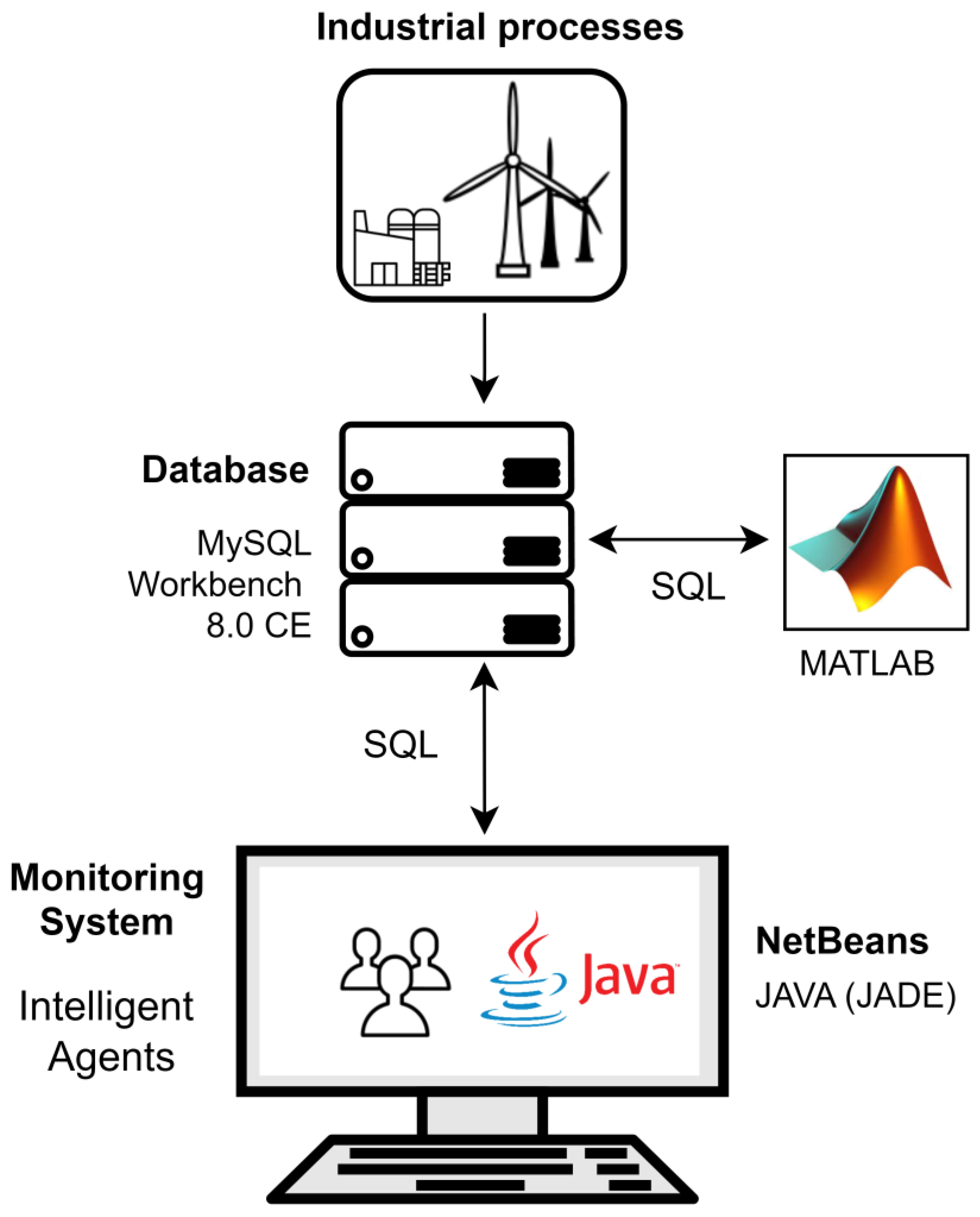
Figure 5 shows the programs used to implement the proposed strategy and how they relate to each other. Data without digital treatment are stored in an Oracle database MySQL Workbench 8.0 CE. These data are preprocessed for the development of ANN models using MATLAB R2019a. MATLAB uses the train function to train neural networks in a file with a (.m) extension. The train function receives in its inputs the input and output data of the neural network and configurations that determine the topology of the neural network, and algorithms used for training, and returns the trained RNA model and other information according to the training criteria provided in the input. Through SQL commands provided in string form to the fastinsert function, the trained model is stored in the database and each RNA model is stored in a different table.

As shown in Figure 5, the monitoring system was implemented in JAVA using the NetBeans 12.6 program with the JADE library. When the intelligent agents are initialized, they load the RNA models from the database through SQL commands.

3.8. General Indicator for Monitoring the Operating Conditions of Industrial Processes

This section presents a general indicator of the health and operational conditions of industrial systems. First, the moving count of the alarms of agents is calculated for a window of time empirically defined by 100 samples according to Equation (11).

$$MSA\left(n\right)={\displaystyle \sum }_{k=1}^{k-100}\left[{\epsilon }_{A_1}\left(n-k\right)+\dots +{\epsilon }_{A_n}\left(n-k\right)\right]$$

(11)

MSA(n) represents the alarm count for all the agents from the agent $A_1$ to $A_n$ for the sample $n$ in the range of 100 consecutive samples, where $n\ge 100$. Each term of the expression ${\epsilon }_{A_1}\left(n-k\right)+\dots +{\epsilon }_{A_n}\left(n-k\right)$ represents the binary alarm output provided by each agent. Subsequently, it is applied to the MSA moving average of 1000 consecutive samples, according to Equation (12). These formulas should be used whenever a new sample of the measurement sample is uploaded to the database.

$$GHCI\left(n\right)=\frac{MSA\left(n\right)+MSA\left(n-1\right)+\dots +MSA\left(n-N\right)}{N},$$

(12)

where $GHCI\left(n\right)$ represents the general health and condition indicator of an industrial plant for the $nth$ sample, where $n\ge N$ and $N$ is the number of samples from the time window used to calculate the moving average.

A systematic evaluation of an industrial plant can be performed by setting a threshold of the moving average value for generating alarms, indicating that a certain number of subsystems are persistently malfunctioning on average. This indicator was developed to simultaneously aggregate the operating conditions of all the subsystems to provide an overview of the industrial plant conditions when several subsystems operate in abnormal situations.

4. Wind Turbine FMEA and Experimental Setup

The method presented in the previous section is applied to a wind turbine to generate a platform for monitoring its operating conditions and health. Thus, as shown in Figure 1, the industrial process represented corresponds to a wind turbine. For the database, a free version of Oracle MySQL Workbench 8.0 CE was used to store the digital data of the wind turbine sensor measurements and the parameters of the ANN models. All information stored in the database is accessed by the intelligent agents through the structured query language (SQL).

The ANNs were written in MATLAB programing language only for training the ANNs to obtain the models of normal behavior. Thus, for convenience, the instructions for saving and updating the models in the database were also developed in MATLAB. In the database are stored all the indispensable parameters to execute the ANNs models, such as input signal normalization constants, number of layers, all synaptic weights, and activation function of each neuron. In this way, the ANNs can be created and trained in any programing environment, requiring only that the parameters of the ANNs are stored in the database in the correct format. The agents were developed in the Java programing language using JADE software agent development platform libraries. Each agent is equipped with its ANN capable of loading and using the same parameters of the ANN stored in the database to process the measurements of the plant signals [21]. In addition, the role of these agents is to monitor the variables of the SCADA system and the temperatures of the various devices of the wind turbine for checking if they are operating within normal values.

Equipment temperatures, due to operating conditions, are also influenced by the internal temperature of the nacelle, which, in turn, is influenced by the variations in the external temperature due to the cycle of day and night. Besides the day-to-day variation, there are significant temperature variations throughout the year in many regions of the world because of climatic conditions and seasons [28]. However, thermal insulation generates a microclimate inside the nacelle because of the heat generated by the equipment. These circumstances can significantly influence the operating conditions and trigger failure modes in components such as the speed gearbox [25]. For these reasons, monitoring the internal temperature of the nacelle and its various parts is particularly important to identify anomalies in the operation of the subsystems and equipment inside the nacelle.

The FMEA was applied to define which are the output variables and which are the input variables for each ANN model. However, before carrying out the supervised training of ANNs, it is necessary to preprocess the data to suppress faulty data that can generate nonoptimized models. The next step was to develop the intelligent agent system. After these processes, the complete fault detection and monitoring system of the wind turbine was obtained, and its performance could be evaluated.

Table 1. Wind turbine parameters.

Parameter	Description
Wind Turbine Model	Horizontal-Axis Wind Turbines (HAWT)
Rated Power	2 MW
Rated Wind Speed	10 m/s
Gearbox configuration	Planetary

shows a few characteristics of the wind turbine studied here.

The following subsection presents further details of the method for signal conditioning applied to wind turbines.

4.1. General Indicator for Monitoring the Operating Conditions of Industrial Processes

Obtaining the models through supervised training requires high-quality data, so preprocessing the digitized data to suppress defective data is very important. So, after the data cleansing step, the database used in this study contains over four years of measurement data corresponding to 17 different variables of a wind turbine. These variables are physical temperature signals, hydraulic pressure, wind speed, blade angle, and electric power produced by the wind turbine.

The data correspond to 262,871 samples for each different variable and the time interval from 10:50:00 on 30 June 2009 to 22:30:00 on 7 September 2014, with an interval of 10 min between the samples. Appendix B shows the main statistical values of the wind turbine signals data at

Table A1. Measured signals’ maximum, minimum, standard deviation, and mean values.

Signal	Maximum	Minimum	STD Deviation	Mean Values
A	78.93	6.38	6.31	63.16
B	86.89	1.81	7.93	42.02
C	94.82	2.36	9.95	53.28
D	65.46	3.61	7.44	35.08
E	202.35	−1.60	13.32	188.76
F	91.10	−4.80	16.34	8.91
G	2081.32	−82.12	715.61	616.68
H	54.48	0.92	8.71	26.87
I	80.09	8.22	7.33	65.25
J	42.59	−4.49	8.33	19.88
K	32.40	0.00	4.23	6.71
L	729.74	0.00	10.52	685.53
M	671.68	−664.12	112.69	−53.17
N	2011.91	−93.57	640.88	617.16
O	33.85	−20.80	8.88	8.30
P	100.00	0.00	42.79	75.87
Q	18.10	0.00	4.78	11.72

.

Some essential aspects that have also been observed in many other industrial systems are considered to evaluate the performance of the proposed monitoring method. The first aspect considered is the need to test the performance of the method by continuously increasing the database size. The second aspect is to verify the performance of the parts of the turbine over the years; thus, throughout the first year of operation, it is expected that all the subsystems will function appropriately; over the second year, deviations from normal behavior, particularly incipient failures, are likely to appear in some subsystems of the wind turbine, and, over the third year, it is expected that more subsystems may show even more significant deviations, indicating the appearance of simple or even catastrophic failures. The third aspect is to suppress the influences of annual periodicity of the meteorological conditions, such as wind speed and temperature that affects all the subsystems of the wind turbine inside the nacelle, and, consequently, the data acquired for training the ANNs. The dataset was used in three different ways in terms of the period and number of samples to consider all these aspects:

• P1: approximately one year, with 52,595 samples;
• P2: approximately two years, with 2 × 52,958 samples;
• P3: around three years, with 3 × 52,958 samples.

The dataset portions P1, P2, and P3 were used to train three different models for each agent and the models were stored in three different databases on the same database server.

The most common problems found in the database of the present study were outliers and data suppression with NaN (not a number). It is necessary to discard signals with large ranges based on NaN.

4.2. FMEA for Selecting the Input Variables of the ANN Models

An FMEA analysis was conducted to avoid the variables that can be physically influenced due to their proximity, to generate models that share signals, and for agents to interact and co-operate to reduce false alarms [25,27].

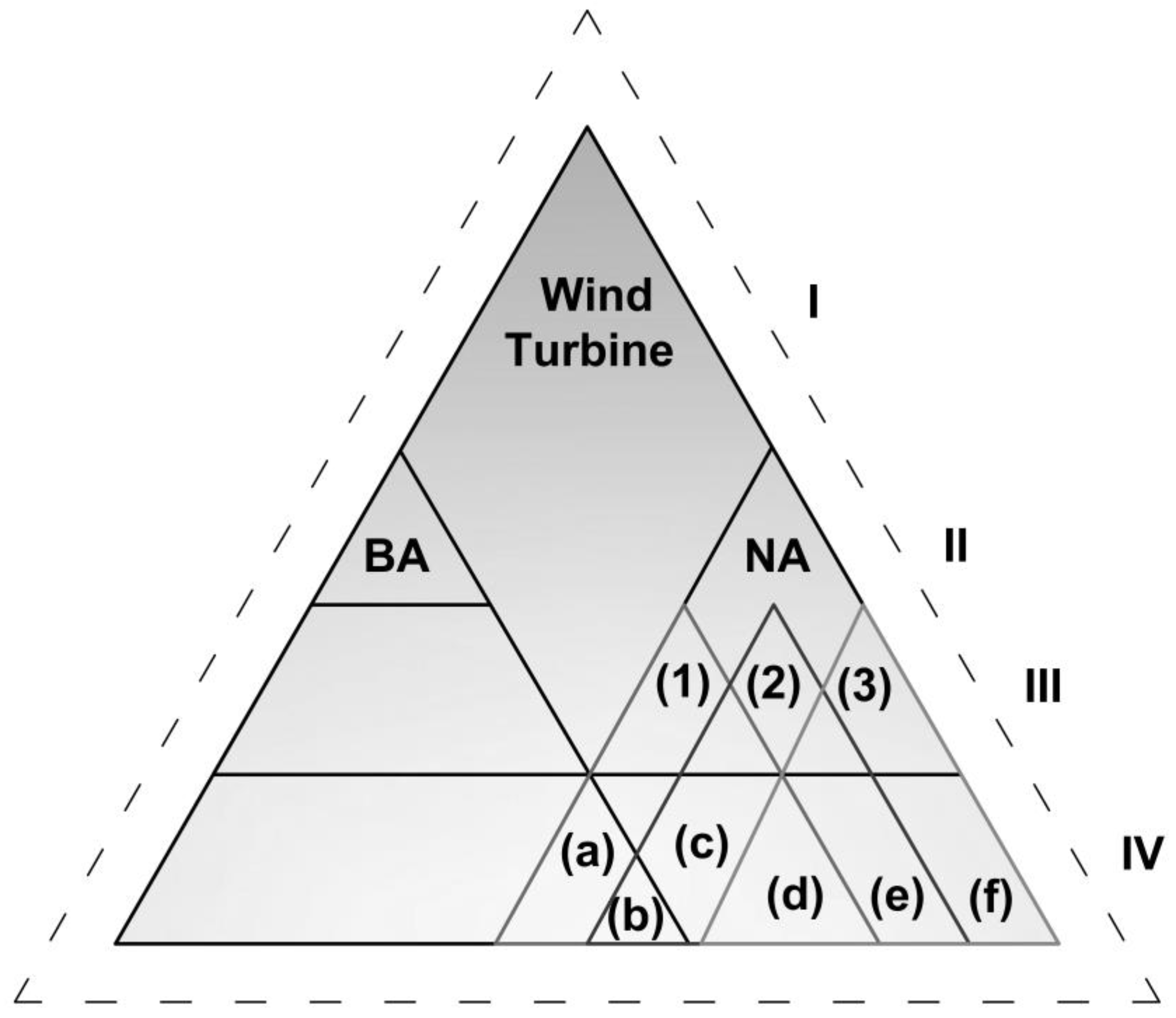
Figure 6 shows a simplified illustration of the hierarchical analysis of the wind turbine systems and components. The four levels shown are:

I—Industrial Process;

II—Systems;

III—Subsystems;

IV—Components of the subsystems.

The two main systems are the wind turbine blade (BA) and the nacelle (NA). Both are represented by triangles, in the internal parts of the vertices. Some parts of these systems are interrelated, as shown by the letters (a) and (b), represented by the mechanical axis that interconnects the turbine blades with the gearbox, generator axis, or hydraulic system.

Figure 6 shows three subsystems of the nacelle:

• (1) Gearbox;
• (2) Electric generator;
• (3) Hydraulic system.

The mechanical interconnections and physical interactions among the subsystems of the nacelle are represented by the following alphabet letters:

• (a) represents the mechanical connection or the interaction of the wind turbine blades with the gearbox inside the nacelle.
• (b) represents the influence of the BA system on subsystem (2), which possibly results from the rotation of the wind turbine blades being transferred to the electric generator, subsystem (2), through the gearbox.
• (c) represents the mechanical connection or interaction among subsystems (1) and (2).
• (d) represents the joint interaction among the three subsystems (1), (2), and (3); thus, the performance of the hydraulic system in the turbine blades can affect the rotation speed of the generator.
• (e) represents only the interaction between subsystems (2) and (3); therefore, this is outside subsystem triangle (1). Here, it can indicate a strong reciprocal thermal interaction between subsystems (2) and (3) if the hydraulic power unit is close to the electric generator (depending on the turbine design).
• (f) represents the components and devices related only to the subsystem (3).

This list is not exhaustive, and other combinations are not shown in this planar figure, such as devices and variables unique to subsystems (1) and (2) that have not been represented.

Table 2. Systems, subsystems, components, and failure modes of wind turbines.

System	Subsystem	Component	Failure mode
Blade Assembly	Blades	Wind turbine blades	blades overspeed
Turbine Nacelle	Gearbox	Lubricant High-speed bearing	overheating
		Main shaft	main shaft overspeed
	Generator	Bearing on the axis coupling side of the generator Bearing on the opposite side to generator axis coupling	abnormal noise overheating
		Slip rings	partial discharges overheating
		Generated power	active, reactive, or apparent power generated with high or low values
	Hydraulic system	Mechanical actuators	overheating low or high pressure

lists the various failure modes of the wind turbine systems, subsystems, and components.

These analyses were performed based on the available variables in the database and the importance of each subsystem in monitoring the wind turbine’s health and its operating conditions [25,43].

The columns in

Table 3. Measured signals, agents, description, and unit.

Signal	Agent	Description	Unit
A	Agent A	Gearbox Oil Temperature (GOT)	°C
B	Agent B	Drive-End Bearing Temperature (GDEBT)	°C
C	Agent C	Non-Drive-End Bearing Temperature (GNDEBT)	°C
D	Agent D	Hydraulic Group Temperature (HGT)	°C
E	Agent E	Hydraulic Group Pressure (HGP)	psi
F	Agent F	Blade Angles (BAs)	°
G	Agent G	Total Power (TP)	VA
H	Agent H	Generator Slip Ring Temperature (GSRT)	°C
I	Agent I	Gearbox High Bearing Temperature (GHBT)	°C
J	-	Temperature inside the Nacelle	°C
K	-	Wind Speed	m/s
L	-	Generated Voltage Effective Value	Vrms
M	-	Reactive Power	VAr
N	-	Stator Active Power	W
O	-	Temperature outside the Nacelle	°C
P	-	Wind Turbine State (ON, OFF)	-
Q	-	Principal Axis Speed	rpm

show the measured signals from the wind turbine, the letters used to identify them, and their physical units. The first nine signals have agents to monitor the temporal variation in the signal; the acronyms are shown in the description column. Thus, the name of each agent coincides with the respective name of the signal that each agent monitors.

According to the method described in Section 3.3 for generic industrial processes, several ANN configurations were tested to select the parameters and topologies for the normal behavior models of nine wind turbine physical variables. For each ANN model, the neural network regression is computed for the training, validation, and testing dataset. Good models are those with a high correlation coefficient close to the unitary value at the testing dataset.

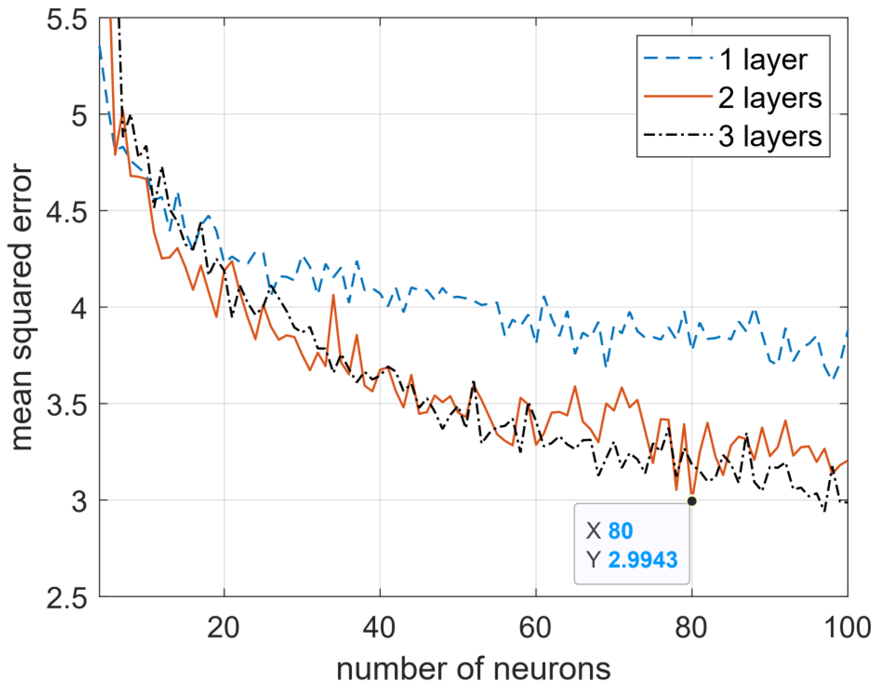
Figure 7 shows the graphs obtained based on the medium quadratic errors for the networks with one, two, and three layers as functions of the number of neurons used to reconstruct a signal using three input signals from the same database of a wind turbine. The three input signals from the neural network are as follows: (i) the temperature of the bearing at the opposite end of the axis coupling of the electric generator, (ii) the sliding ring temperature at the generator, and (iii) the temperature inside the nacelle that is used to reconstruct the signal temperature of the gearbox oil. The topology of two layers with 80 neurons is as efficient as the topology with the same number of neurons in the three-layer topology. Thus, it is more appropriate to use a simpler topology with similar efficiency.

The same procedure described in this subsection must be performed to develop other optimized models with other inputs or outputs. The optimized models obtained are used in the next step in which the strategies for false alarm detection are established.

Table 4. Agents, estimated signals, and ANN models.

Agent	Estimated Signal	Model	ANN Topology
Agent A	$\widehat{A}$	MA(C, H, J)	40:40
Agent B	$\widehat{B}$	MB(H, D, J)	33:34:33
Agent C	$\widehat{C}$	MC(I, H, J)	33:33:33
Agent D	$\widehat{D}$	MD(A, B, F)	36:36
Agent E	$\widehat{E}$	ME(B, A, J, F)	16:16:16
Agent F	$\widehat{F}$	MF(H, B, E, K)	51:50
Agent G	$\widehat{G}$	MG(B, F, K)	51:50
Agent H	$\widehat{H}$	MH(A, I, C)	24:24:23
Agent I	$\widehat{I}$	MI(H, D, G)	32:32:31

presents all the agents developed for this case study, the estimated signal variable, and their respective ANN models and topologies. The input variables presented for each model represent the input layer of the corresponding ANN; thus, the topologies shown in the table correspond only to the hidden layers, with the output layer having only one output signal. Each agent has its model that is expressed according to Equation (3). A description of each input of the agent signal is presented in Table 3.

4.3. Strategy for Error and Alarm Generation, and MAS for Wind Turbines FMEA

The method presented in Section 3.4 was applied to verify the performance of the turbine as it ages.

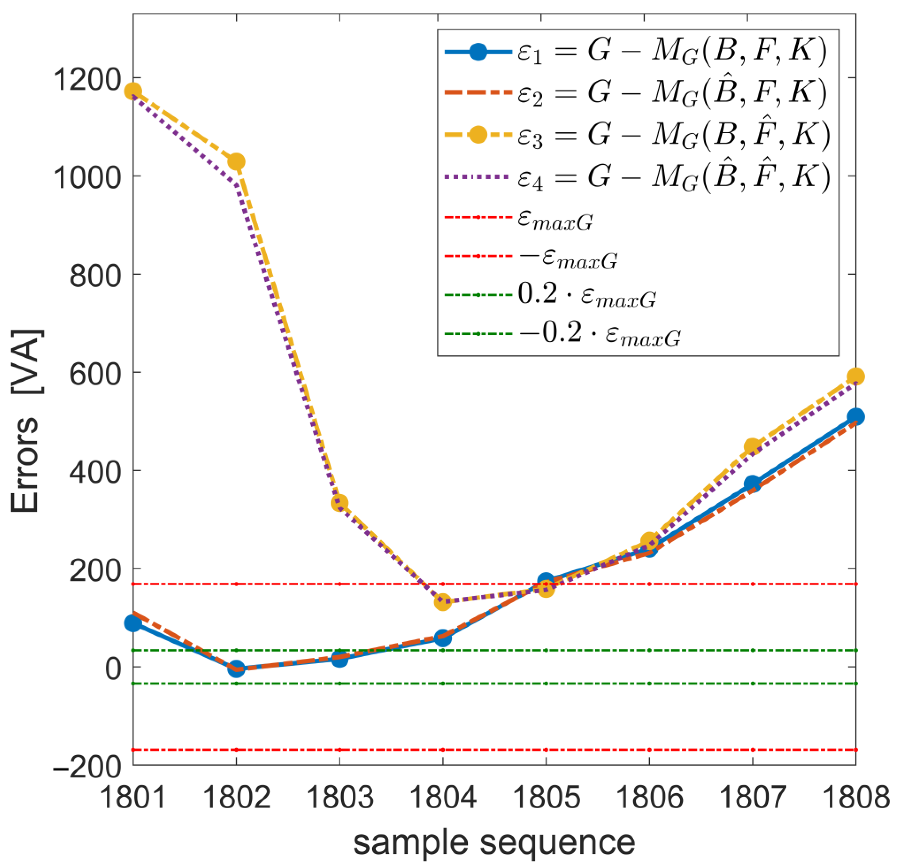
As an illustrative example, Figure 8 shows two samples (1802 and 1803) that satisfy the conditions for the rejection of the error prediction of the agent with the normal behavior model F (in charge of monitoring the F signal). The most prominent error occurs when the estimated value of $\widehat{F}$ is used as input of the model $M_G\left(B,\widehat{F},K\right)$.

When the estimated $\widehat{F}$ value is used as an input to model $M_G$, it causes a significant estimation error of model $M_G$ $\left({\epsilon }_3\right)$; therefore, the estimated value of $\widehat{F}$ is not accurate, and it is a false alarm of the $M_F$ model.

The same logic can be applied to the $M_B$ model; in other words, the $M_G$ model can be used to assess whether the $M_B$ model generates a high estimation error of the normal behavior of signal $B$, in this case ${\epsilon }_2$.

This method calculates the error threshold for each ANN model for three different training intervals (one year, two years, and three years).

Table 5. Agent activation thresholds for one, two, and three years.

Model	Threshold for:			Error
	1 Year	2 Years	3 Years
Model A	3.864	4.511	9.864	${\epsilon }_{maxA}$
Model B	5.565	7.318	7.782	${\epsilon }_{maxB}$
Model C	6.392	7.537	7.633	${\epsilon }_{maxC}$
Model D	6.164	8.975	8.394	${\epsilon }_{maxD}$
Model E	10.891	11.339	11.735	${\epsilon }_{maxE}$
Model F	17.752	16.997	16.577	${\epsilon }_{maxF}$
Model G	176.638	180.435	193.269	${\epsilon }_{maxG}$
Model H	8.702	10.294	10.232	${\epsilon }_{maxH}$
Model I	5.890	6.772	6.998	${\epsilon }_{maxI}$

lists the calculated error thresholds corresponding to the normal operating conditions of the various wind turbine subsystems. The error column presents the maximum error acronym for each model.

Here, we apply the method presented in Section 3.5., establishing the interaction among the intelligent agents to generate an MAS to monitor the wind turbine. Thus,

Table 6. Agents, estimated signals, and ANN models.

Agent	ANN Model	Committee
Agent A	MA(C, H, J)	MD, ME, MH
Agent B	MB(H, D, J)	MB, ME, MF, MG
Agent C	MC(I, H, J)	MA, MH
Agent D	MD(A, B, F)	MB, MF
Agent E	ME(B, A, J, F)	MF
Agent F	MF(H, B, E, K)	MD, ME, MG
Agent G	MG(B, F, K)	MC, MD
Agent H	MH(A, I, C)	MA, MB, MC, MF, MI
Agent I	MI(H, D, G)	MC, MH

shows all the MAS committees.

In the analysis of the agent committee, a given wind turbine signal measurement is considered a false alarm when at least one of the agents classifies it as a false alarm. This final analysis is performed by the synchronizing agent because it receives the output of all the agents.

4.4. JADE agent Architecture for Wind Turbines

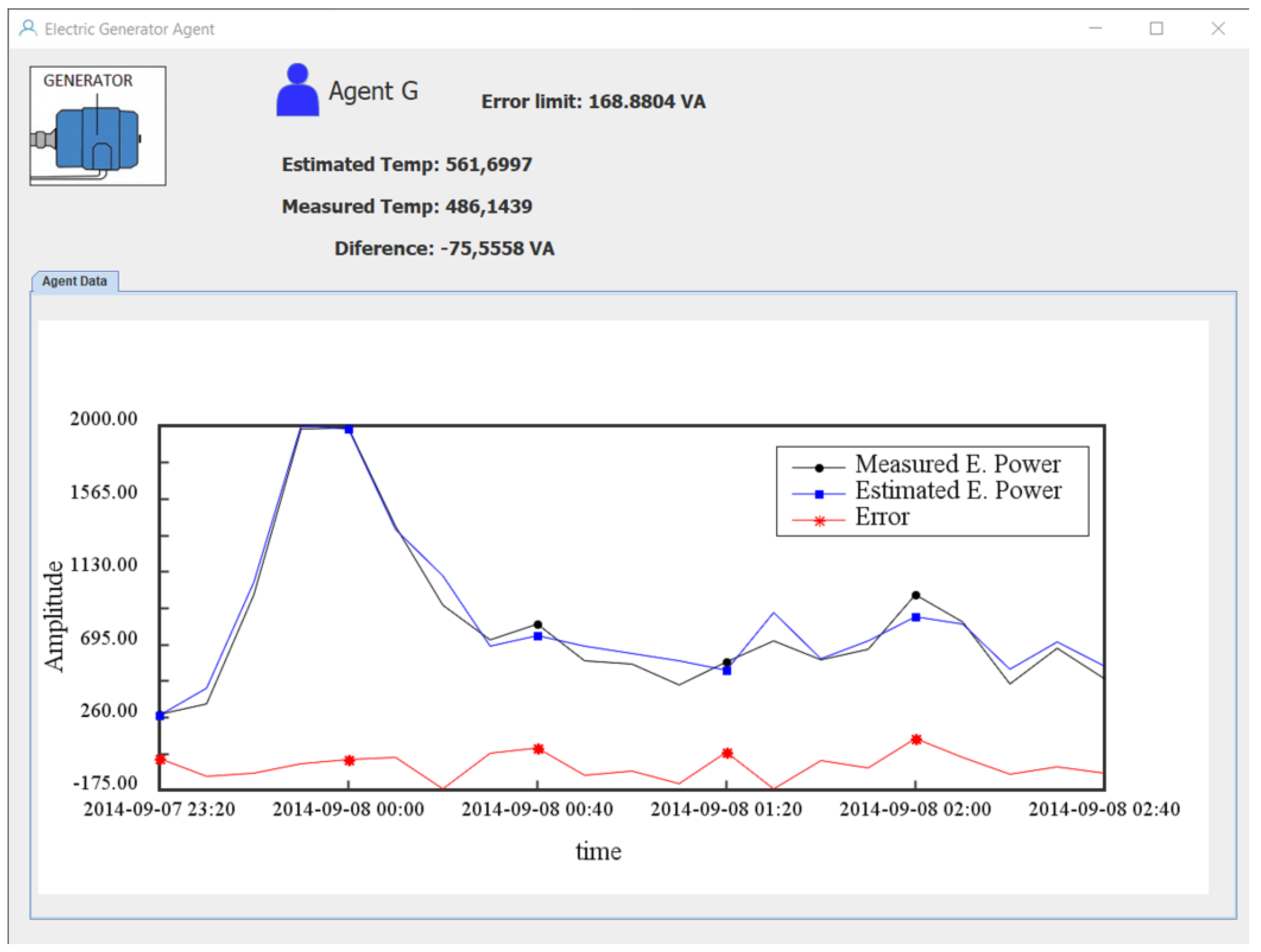
The definition of the architecture within JADE applies the basic principles presented in Section 3.6. According to Table 4, nine agents were designed with a similar graphical interface as show in Figure 9.

Thus, it is possible to visualize the measured variables, estimate the variable value obtained by the ANN model for each sample, and determine the estimation error, as shown in Figure 9.

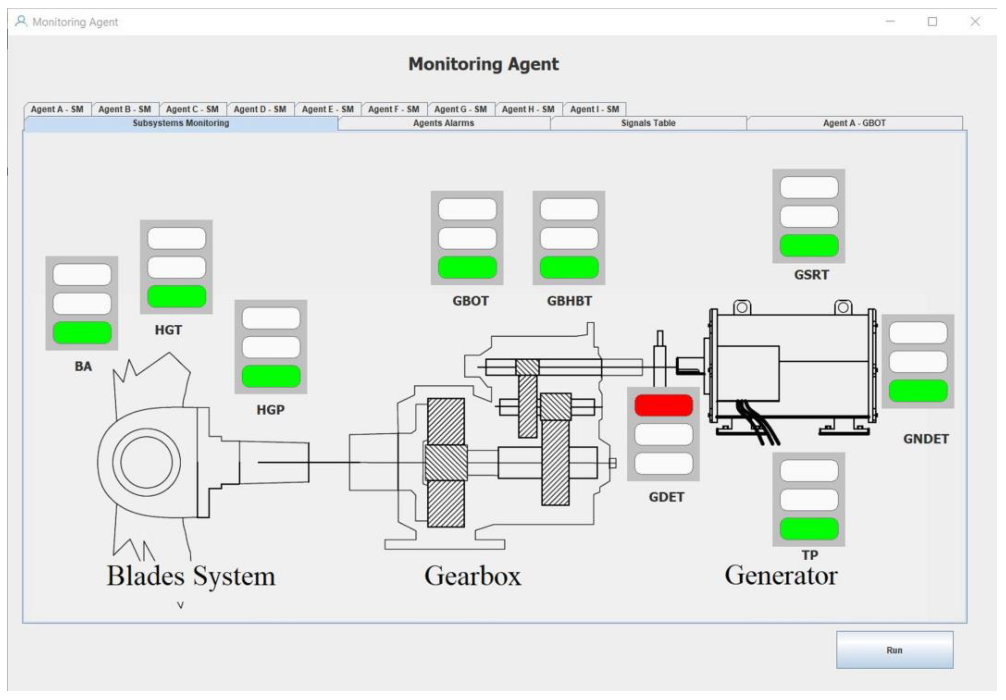
Figure 10 shows the graphical interface of the synchronizer or monitoring agent. Through this agent graphical interface, the operator can visualize the result of the application of ANN models of each agent through nine traffic lights, one for each agent. Table 5 shows the meaning of each acronym related to each agent; each model has an activation threshold equal to a maximum limit. For errors greater than the threshold, the red traffic light shows high errors compared to the value expected by intelligent agents. However, for values up to 20% of this limit, the green traffic light represents a tiny error. If a committee agent is in a green state, it can judge the output of another agent (whether it is a false alarm). For errors between 20% and 100%, the yellow light represents a moderate error.

For false alarm detection, the first agent detects that the signal it monitors has a discrepancy above the expected threshold, as shown in Figure 10; in this case, the drive-end bearing temperature (GDEBT) is red-flagged. The agent that is part of the committee that can check if it is a false alarm signaled by agent B (shown in Table 3) is the $M_G$ that should have a low output error; therefore, it should correspond to green light.

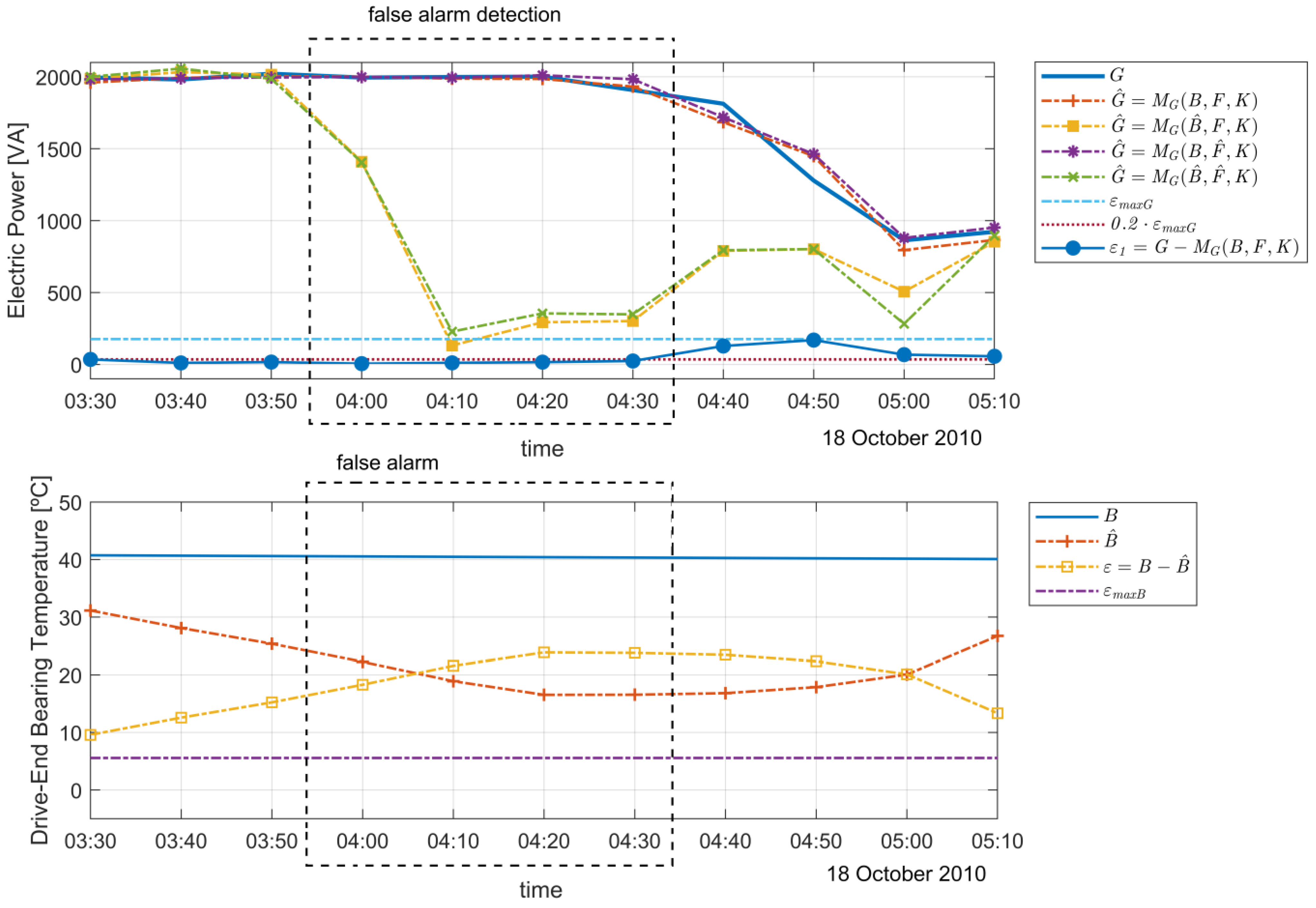
As an example of false alarm detection, Figure 11 shows the values of the signals analyzed by agents B and G that satisfy all the conditions presented in Section 3.5.

As shown in Figure 4, agent G can check whether agent B has triggered a false alarm. Thus, Figure 11 shows all the conditions under which agent G detected four false alarms at specific intervals from 04:00 to 04:30, and agent G did not show any significant difference with respect to the real and estimated power level that remains high with the combination of the signals B, F, and estimated F ($\widehat{F}$) used as input of agent G. However, after the four alarms were detected, agent G lost the ability to evaluate the signal, as it itself presented a model estimation error above the threshold value, ${\epsilon }_1$. In the same graph of Figure 11, referring to the variable GDEBT, all the visible points before and after the dotted rectangle are examples of true errors, according to the criteria and limits set for the agent B, where the temperature estimation error $\epsilon$ ($B-\widehat{B})$ tends to increase, since, with the reduction in the generation power, it is expected that the temperature of several subsystems and components will decrease.

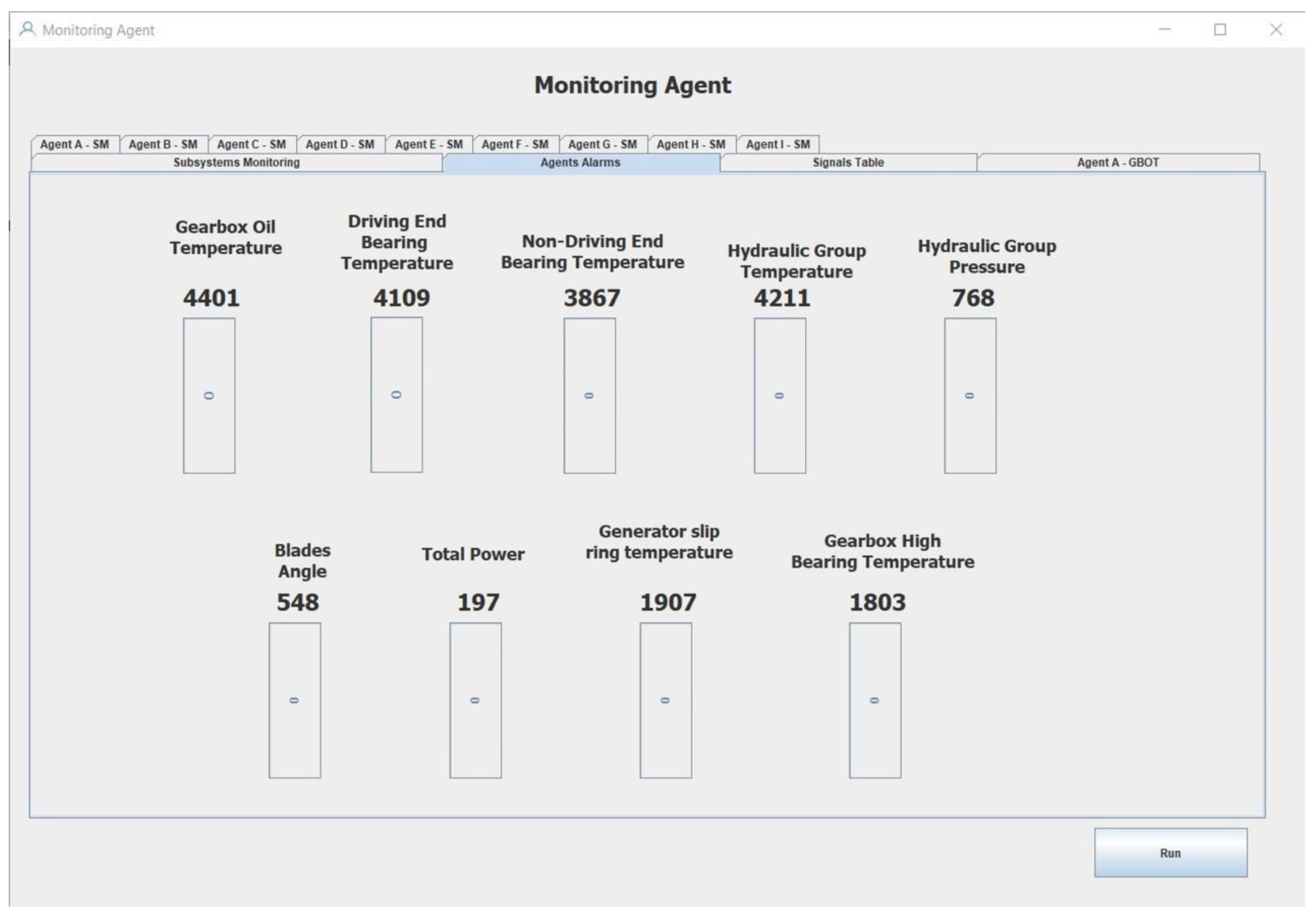
The alarm count related to an agent is stored in a table in the synchronizing agent that acts as an event log.

5. Results and Discussion

In the data cleaning step of the preprocessing, temperature data from the wind turbine transformers were discarded, because large portions were incomplete, including energy measurements among others. The neural network input data were also normalized by training function. Thereafter, the method for monitoring and reducing false alarms in industrial systems was applied to a wind turbine. Thus, the MAS processed the wind turbine data for normal behavior models generated for three different time intervals, always starting from the beginning of the time series:

• Data for first-year training;
• Data for first- and second-year training;
• Data for first-, second-, and third-year training.

The agents analyze the measured signals from the wind turbine to detect false alarms at the same measurement frequency as the SCADA system (10 min), thus providing the operating conditions for a short period through the traffic lights. One of the important results is that it was not possible to verify the performance of the parts of the turbine over the years due to aging, because the available data are from the early years of the wind turbine, and it is a relatively short period compared to the turbine lifetime.

Figure 12 shows the number of alarms accumulated during the entire time series of all the signals monitored by the agents equipped with the ANN models with one-year training. Even though, in the variable selection phase through the FMEA, we try to reduce the influence of nearby physically monitored variables, in these waveforms, we can see that, in some moments, some curves grow simultaneously, which demonstrates the influence of operating conditions and environmental conditions on many monitored variables.

Among the four variables related to the electric generator of the wind turbine, three variables, nominally, B, C (bearing temperatures), and H (collector ring temperature), show high growth in error counts, and G (total power) shows one of the lowest growths of all the signals.

In the hydraulic system, it is essential to observe that the evolution of the number of accumulated alarms for temperature D (temperature of the hydraulic subsystem) is more pronounced than that for pressure E (pressure of the hydraulic subsystem), which has the smallest growth. This is because of the stable characteristics of the hydraulic pressure in almost any operating condition.

In the gearbox, variable A (oil temperature) shows a similar evolution to variables C (generator temperature variable) and D (hydraulic system temperature variable).

Thus, the temperature-related variables accumulated the most alarms in all systems and were the most deviated relative to the normal operating behavior.

The agent group can evaluate the sensitivity of the models and the quality of the model inputs. Thus, it is possible to assess the impact of the variable change using the estimation results of each model related to an agent group.

Table 7. Agents, estimated signals, and ANN models.

Variable	Alarm Reduction
	1 Year	2 Years	3 Years
Variable A	5.818%	11.651%	17.704 %
Variable B	17.749%	18.565%	15.186%
Variable C	3.716%	6.845%	4.892%
Variable D	7.034%	3.039%	5.098%
Variable E	5.331%	5.061%	14.316%
Variable F	20.562%	17.449%	9.958%
Variable G	0.358%	0.147%	0.066%
Variable H	37.737%	26.588%	22.505%
Variable I	20.446%	16.373%	26.247%

shows the error reduction when agent committees are applied to analyze wind plant signals with models trained over one year, two years, and three years, with data other than the ANN training data.

The various agent groups achieved a significant reduction in the number of alarms for some components for which it was challenging to obtain more accurate models, such as the coupling axis end bearing temperature (variable B), blade angle (variable F), generator slip ring temperature (variable H), and high-speed side bearing temperature of the gearbox (variable I).

Figure 13 shows the total number and alarms for each variable monitored by the wind turbine agents. The alarms provide information on the medium-time operating conditions generated when an uninterrupted sequence of five alarms occurs (50 min). This strategy contributes to a significant reduction in alarms and serves to assess the operating conditions of the wind turbine more carefully.

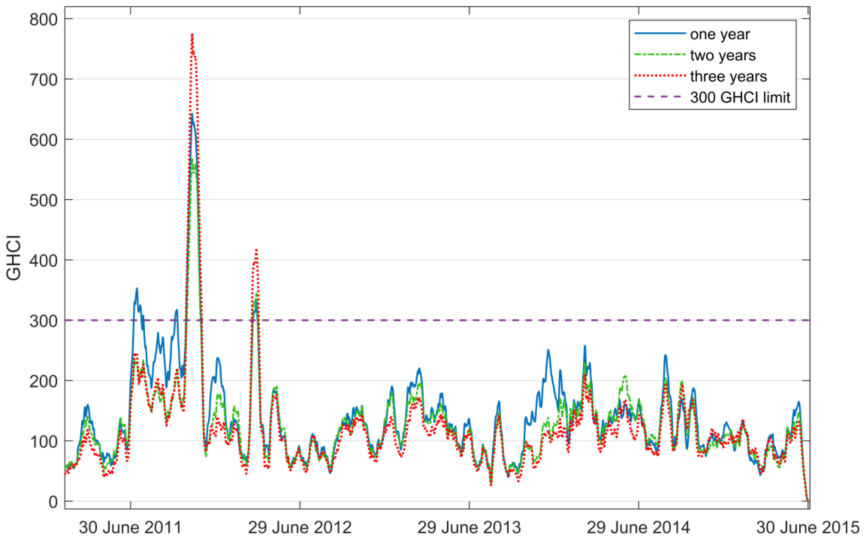
Figure 14 shows a particular time interval of the curves obtained for the wind turbine from the General Health Conditions Indicator (GHCI) for all the agents equipped with normal behavior ANN models with one, two, and three years of training, as shown in Section 3.7. Although the training data have been partitioned to reduce the influence of the annual periodicity of the meteorological conditions, such as wind speed and temperature, the three waveforms show the annual periodicity of the aggregated alarms triggered by all agents.

Using this curve, it is possible to establish a threshold for determining when preventive maintenance should be performed, as shown in the long term, when various subsystems operate outside the expected values. Because the error count is performed in the interval of 100 consecutive samples, this indicator shows, in simplified form, that, for every 100 units on the vertical axis, there is an equivalent subsystem with many persistent alarms. Thus, as can be seen in the graph, three peaks have at least three systems with many deviations (above 300 units) from normal operating conditions, but they can only be detected by the agents equipped with the ANNs trained with only the first year of time series data. This result is expected because the longer the training time, the higher the probability of operating under conditions different from the initial conditions. This shows the importance of updating the models periodically to reduce false alarms as the industrial system ages and settles into new normal operating conditions. Networks trained with three-year data have already incorporated in their model larger ranges of variable values that are considered normal; however, this behavior, when compared with data from the first year, shows a reasonable deviation in the turbine behavior. Thus, the update of the models should be performed carefully, such that the ANNs are not trained with data from periods when the turbine is at the end of its useful life because it may lead to the consideration of typical signals from deteriorated subsystems and with severe anomalies as normal behavior [10].

A rapid increase in the alarm count within a short period may mean that there are damaged sensors, communication problems between the sensors and the data acquisition system, or failure in operating conditions of the monitored devices. Similarly, the occurrence of high alarm rates in many of the subsystems that constitute the wind turbine is a significant sign that the wind turbine is at the end of its useful life [44].

The detection of false alarms can isolate the root cause of the disturbance variables or reveal which variables or models are reliable and consistent. The estimation models reveal the variables that cause higher cumulative alarms. Thus, they can indicate models that generate reliable estimates and their impacts on other models.

In [38], a statistical method was used to reduce the number of false alarms by adjusting the tolerance range of normal behavior. In contrast, this study used a method with neural network models with intelligent agents that collaborate with each other; this extends the reduction in false alarms beyond the capacity of each ANN model. Thus, the measurements are processed in their best fits of the normal behavior threshold.

Thus, this study provides a procedure that can be followed to establish consistent models through hierarchical analysis with FMEA in a wind turbine, and these steps can be extended to several industrial systems. It objectively demonstrates the interaction of intelligent agents via ANNs. Finally, it aggregates the health of all subsystems of an industrial process in a single indicator. These are significant advances as compared with the reference study [45]; although the prior study presents several intelligent agents for failure detection, it does not present an objective method of aggregating information between agents to increase monitoring efficiency, reduce false alarms, or provide a general indicator of wind turbine health. As the intelligent agents have the characteristic of distributed artificial intelligence, they can be reused in other wind turbines of the same farm with similar characteristics, mainly in the initial stages of operation, and, later, they can receive new models of ANNs trained with the accumulated data of the own plant and neighboring plants, since, with the proximity, they may be subject to the similar electrical and climatic operating conditions.

According to Rubert et al. [3], maintenance costs are high, and false alarms can generate unnecessary costs, as they can lead to the unnecessary activation of maintenance teams to perform checks at the installation site of the wind turbine, resulting in significant expenses. Thus, the reduction in false alarms contributes to cost reduction and improves the economic viability of the project.

6. Conclusions

This paper presents a method to improve the safety of diagnosing the health and operating conditions of a wind turbine by using an MAS trained with data of short, medium, and long term (one year, two years, and three years, respectively). Thus, it aggregates several models for normal behavior estimation through a computing platform of specialized agents that facilitates updating and adapting the models for new turbines. In addition, they can also be extended to other industrial systems.

The agents form various co-operating groups as committees that assess the processing outputs of other agents and reject erroneous estimates of the monitored wind turbine signals. Therefore, these groups of intelligent agents facilitate false alarm reduction. Consequently, they have an enormous potential to limit the requirement of maintenance and improvement in the degree of accuracy in applying maintenance techniques based on operating conditions, thereby reducing costs in the medium and long term.

By employing the proposed methodology, it was possible to reduce the total number of false alarms by more than 20% in the most critical subsystems, for example, the axis coupling end generator bearing temperature, blade angle, generator slip ring temperature, and high-speed side bearing temperature of the gearbox, over the three years of analysis. Consequently, it reduces the frequency of maintenance requests that are more likely to be triggered according to the long-term indicators shown in Figure 14. Although, annual periodicity of the meteorological conditions with the more severe environmental conditions in some months leads the turbine to operating more often outside the normal behavior and the GHCI threshold must be a little higher.

The developed platform based on distributed artificial intelligence and communication reduces the need for a large communication bandwidth and expensive computers because most of the processing is local. The distributed platform also increases the robustness of the system because, even when a few agents collapse, others remain in operation.

Thus, it is possible to enhance the existing wind turbine monitoring systems with new indicators of health and operating conditions by deploying a distributed integrated system composed of intelligent agents.

A limitation of the present study is that the data measurement time does not cover advanced stages of wind turbine aging, wherein significant amounts of anomalies, catastrophic failures, and maintenance that would affect the measurement are expected, allowing for a better evaluation of the developed models.

Future research may include the development of models with other computational intelligence techniques integrated with ANN models and establishing normalized parameters that allow the transfer of learning or direct application to several different types of wind turbines without the need to remodel and retrain.