Numerical Investigation of the Effect of Hub Gaps on the 3D Flows Inside the Stator of a Highly Loaded Axial Compressor Stage

Abstract

Both the compressor performance and the 3D flows inside the stator passage are significantly impacted by the stator hub gap. The interplay between leakage flow and corner separation within a cantilevered stator of a highly loaded, low-speed axial compressor with a succession of stator hub gaps was examined numerically in this paper. Firstly, the simulated results were compared with the measured results, including the compressor characteristics, the 3D flow structures, and the flow fields at the stator outlet. The results revealed that the used CFD solver, as well as the corresponding setup, can reproduce the flow not only in terms of the trend along with the stator hub gap, but also in terms of the specific scale of the 3D flow structure. Hence, it is feasible enough to be applied in the present investigation. Secondly, the flow mechanisms of the interplay between the corner separation and the leakage flow with different stator hub gaps were analyzed. It was found that the velocity of the leakage flow is the key parameter that dominates the flow structures as well as the compressor performance. Additionally, a simple metric was proposed to be used to choose the optimum stator hub gap. By comparing our results with those from published research, this metric was proven to be feasible. Finally, it is also discussed how the stator hub gap affected the stator inlet flow and rotor performance. It is demonstrated that the stator passage flow blockage can affect the upstream flow field. As a result, the performance of the rotor tends to vary in the opposite direction to that of the stator.

1. Introduction

The cantilevered stator is one of the frequently used configurations in axial compressors. In contrast to the shrouded stator, the interaction of the corner separation and leakage flow is the primary feature of the cantilevered stator flow. The leakage flow produced by the space between the blade tip and the endwall usually flows in the opposite direction to the secondary flow in the wall boundary layer of the cantilevered stator. This can weaken the corner separation by preventing the low energy flow from moving to the corner that is bounded by the blade suction surface and the endwall [1,2,3,4].

Many studies have been conducted about the detailed flow mechanism of the interplay between these two secondary flows. Many studies have suggested that the corner separation is weakened by the leakage flow, which suppresses the migration of the low energy flow [1,3,5,6,7], while Dong et al. [8] thought that the leakage flow has an energizing effect on the low energy flow in the corner, which is the primary reason for the suppression of corner separation, and Gbadebo et al. [9] noted that the elimination of the corner separation is caused by the suppression of the horseshoe vortex in the leading edge. In total, there is still no uniform conclusion on this question. However, one thing is certain: the stator’s performance is significantly influenced by the stator hub clearance scale, and in most circumstances, there is an ideal value that results in the best stator or compressor performance [3,10]. Lakshminarayana and Horlock [3] pointed out that in the case of the optimal gap, the secondary flow and the leakage flow cancel each other out, which also shows that their intensities are basically equal; Sakulkaew et al. [11] found that the balance of flow mixing loss and tip clearance viscous loss resulted in an ideal clearance for the rotor tip of an industrial gas turbine. In addition, leakage flow can enhance compressor performance and reduce the corner separation of the stator hub, as demonstrated by many researchers [9,12,13]. George et al. [7] found that when this gap size is very small, clearance flow tends to exacerbate corner separation. However, how to choose this optimum stator hub gap is still an unsolved problem.

In paper [14], a thorough experimental analysis was carried out in a cantilevered stator of a highly loaded axial compressor from the perspective of these two problems. The stator hub gaps of four different stator configurations—0% (shrouded), 0.25%, 0.5%, and 1% blade height—were studied. Both the five-hole probe and oil-flow visualization were utilized to measure the intricate flow fields in order to clearly grasp the evolution of the 3D flow structures inside the stator with different mass flow conditions and stator hub gap sizes. The impact of the stator hub gap size on compressor performance was also covered. However, due to the lack of detailed flow information, such as the flow structures inside the stator passage and the velocity and pressure of the leakage flow, the flow mechanism of interplay between the corner separation and leakage flow was not revealed, and the discussion about the optimum stator hub gap was not displayed.

The flow within this compressor with different stator hub gap scales will be simulated in this paper using the CFD approach. By comparing the compressor performance, the flow structures inside the stator passage, and the flow fields at the stator outlet, the selected CFD solver and the corresponding setup used in this paper were proven to be feasible enough to analyze the detailed flow mechanisms of the investigated compressor. It is anticipated that this study will provide a greater understanding of the mechanisms of interaction between corner separation and leakage flow inside the cantilevered stator, and a metric applied to choose the optimum stator hub gap will be obtained. In addition, one question about the effect of the 3D flow structures inside the stator passage on the upstream flow fields is usually neglected when the study is conducted in compressor stages. Hence, in this paper, this question will be also discussed.

2. Investigated Compressor

The investigation was conducted on a compressor designed based on the low-speed large-scale axial compressor (LSLSAC) test facility of Beihang University, as shown in Figure 1. The casing diameter is 1 m, with a hub-to-tip ratio of 0.6. Three blade rows compose the compressor stage, i.e., the inlet guide vane (IGV), the rotor, and the stator. Among these, the IGV is shrouded, the rotor has a tip clearance of 1% blade height, and both the rotor and the stator employ the controlled diffusion airfoil (CDA) and are almost radially stacked. The stator may be shrouded or cantilevered. In addition, the stator hub is stationary while the rotor rotates at 1100 RPM. More detailed design parameters of the compressor can be seen in Yu [15].

In the previous paper [14], the flows inside the stator with four different hub clearances, i.e., 0%, 0.25%, 0.5%, and 1.0% blade height (denoted as 0.00 τ, 0.25 τ, 0.50 τ, and 1.00 τ), were experimentally investigated. Except for the compressor characteristics, both the five-hole probe and oil-flow visualization were used to capture the 3D flow structures inside and outside the stator passage. Those results provided the validation data and the analysis basis for this paper. In the present paper, six compressor configurations with different stator hub clearances (0.00 τ, 0.25 τ, 0.50 τ, 1.00 τ, 1.50 τ, and 2.00 τ) were simulated.

3. Numerical Setup

3.1. CFD Solver

As discussed in previous works [16], using the commercial software package ANSYS CFX, the widely used eddy viscosity models have been assessed for simulating large-scale tip vortices and separating flows in a low-speed axial compressor, which is similar to the investigated compressor in the present paper. The results showed that the two-equation eddy viscosity models were much more suitable for simulating the complex vortex flows in compressors with respect to both computation accuracy and consumption. Hence, numerical simulations in the present work were also computed using the ANSYS CFX flow solver (version 17.1).

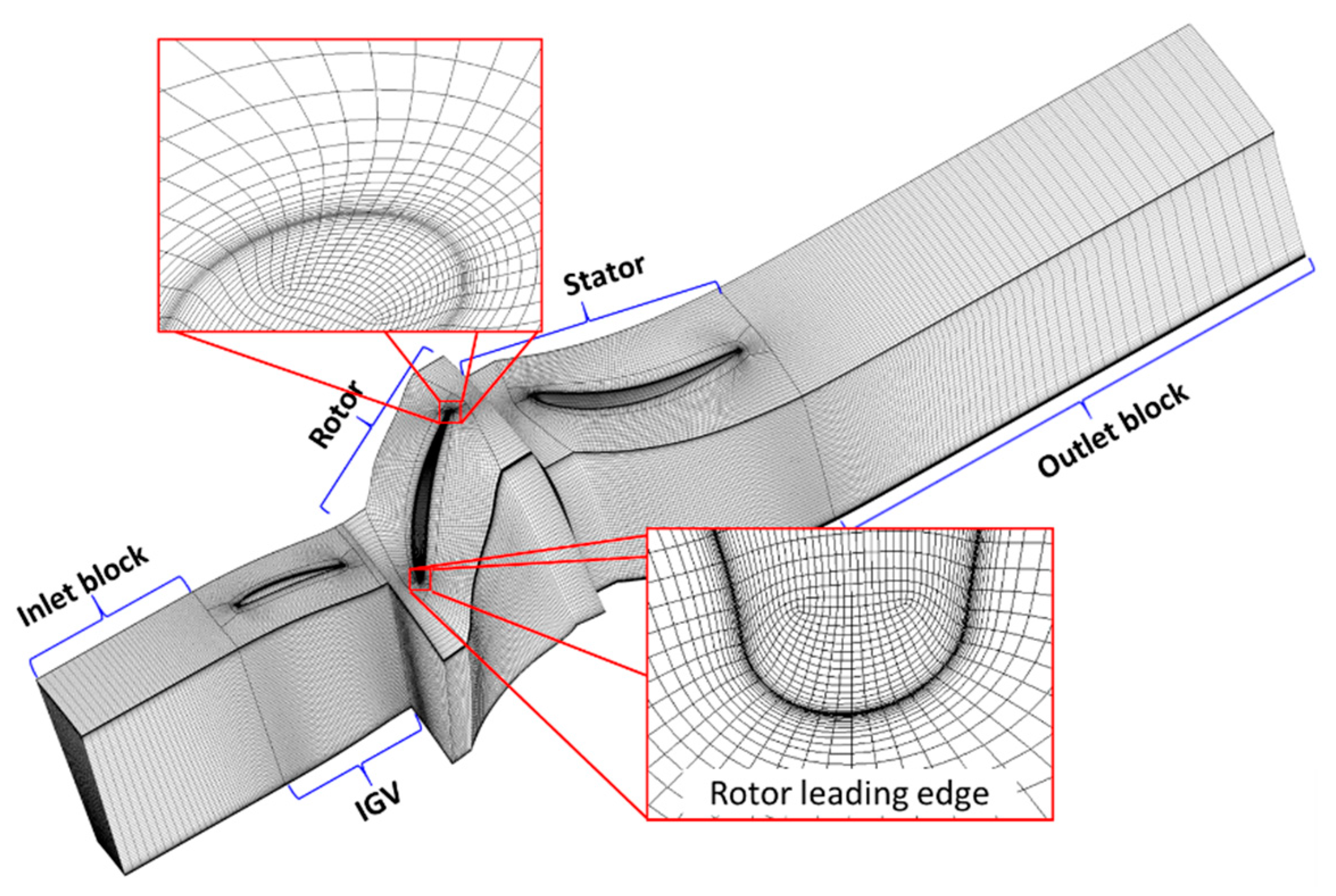
3.2. Grid Generation

According to the compressor’s geometry, computational grids were generated using the commercial software package Numeca IGG developed by Dener and Hirsch [17]. The grids for each of the three blade rows were generated separately. As shown in Figure 2, for all the three blocks with a blade, H-O-H grids were used on the main blade regions. In the clearances, including the hub gap of the stator and the tip gap of the rotor, H-O-type grids were used. These consist of an inner H-block and an external O-block. Upstream to the IGV block, the inlet block was set to the length of two times the IGV blade chord. Moreover, downstream to the stator blade block, an outlet block of 3.5 times the stator blade chord was used. This was to ensure the separated flow structures decayed uniformly when leaving the computational domain.

The grid independence analysis was also carried out in order to rule out the influence of the grids on the simulation. Additionally, when the number of grids was increased, the compressor characteristics and the spanwise distribution of flow parameters of the upstream and downstream blade rows were studied. Finally, for the research, a grid with 1.28 million nodes for the rotor and 1.11 million nodes for the stator was selected.

3.3. Boundary Conditions

For the flow through the test rig, the Mach number was relatively low (less than 0.2). Therefore, in the current simulations, ideal gas law with constant specific heat was employed. Additionally, for the inlet boundary, static temperature, total pressure and flow direction were specified. The static temperature was set as 288.15 K for the standard atmosphere condition. The flow direction was set as normal to the boundary, i.e., axial inlet flow. The total pressure was specified using a circumferential averaged radial profile obtained from the experimental results.

Additionally, adiabatic wall conditions and non-slip surfaces were used for all solid surfaces. The pitchwise direction imposed periodic boundary requirements. The rotor block’s coordinate frame was configured to rotate at 1100 revolutions per minute. This was the same rotational speed of the compressor that was adjusted for the experiments. Accordingly, the casing wall in the rotor block was set as the counter rotating wall. Moreover, for the interface between the IGV and the rotor blocks, and also between the rotor and stator blocks, two mixing-plane models were used.

3.4. Turbulence Model

As discussed in previous works [16], two-equation eddy viscosity models were much more suitable for simulating the complex vortex flows in compressors with respect to both computation accuracy and consumption. In this paper, the standard k-ω model was chosen, as it can capture more accurate 3D flow details than the standard k-ε model, and can result in a better convergence than the SST model. More details about the standard k-ω model can be seen in [18,19].

3.5. Numerical Schemes and Convergence Criteria

Numerical schemes can significantly affect the convergence performance. A combination of low-order schemes for advection terms can possess robust convergence, but may also result in higher numerical diffusion and then smear out detailed flow structures. Hence, a combination of second-order spatial and temporal numeric values were selected for all the transport equations. To ensure convergence, for all the simulations, not only the default parameters, such as the mass and momentum residuals, etc., but also extra self-defined parameters, such as compressor pressure ratio, efficiency, inlet mass flow rate, and inlet and outlet flow imbalance, were monitored. Only results with RMS residuals of P-Mass lower than 10-6 and differences between the inlet and outlet flow masses smaller than 0.1% were included in the investigation.

4. Numerical Results

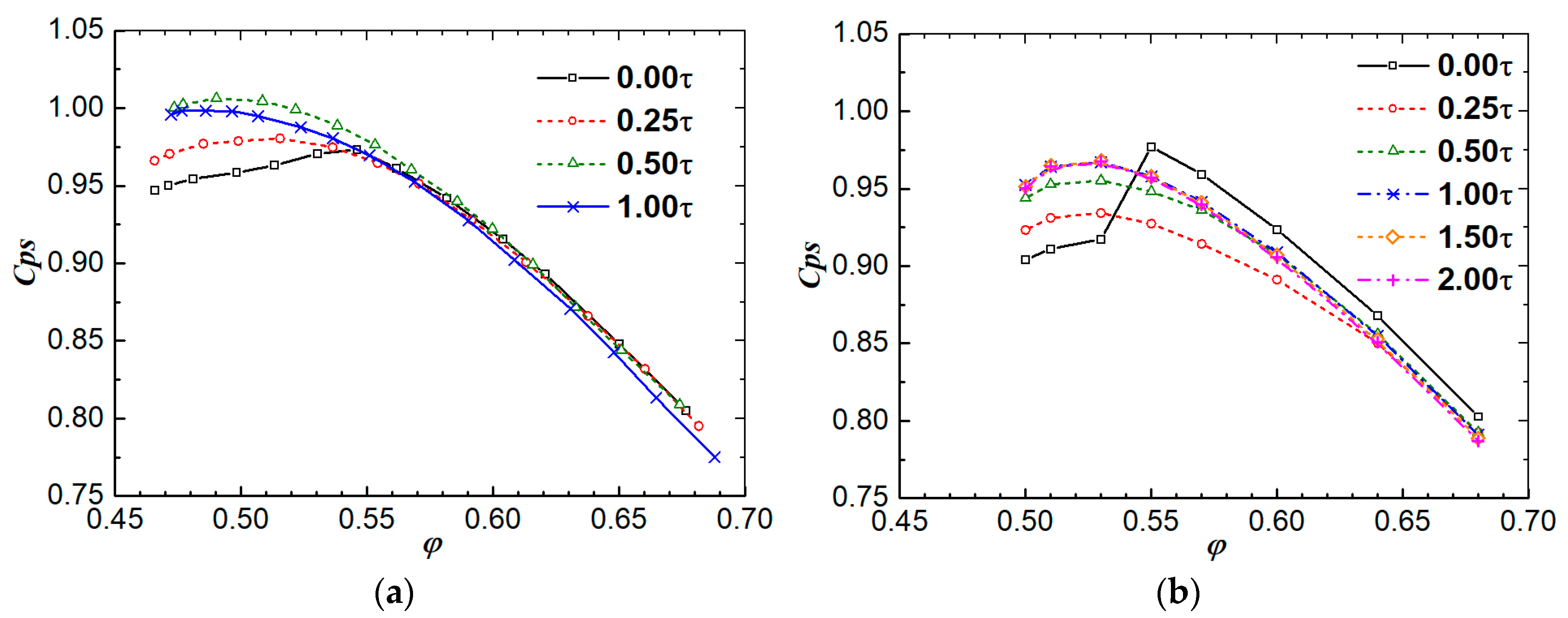
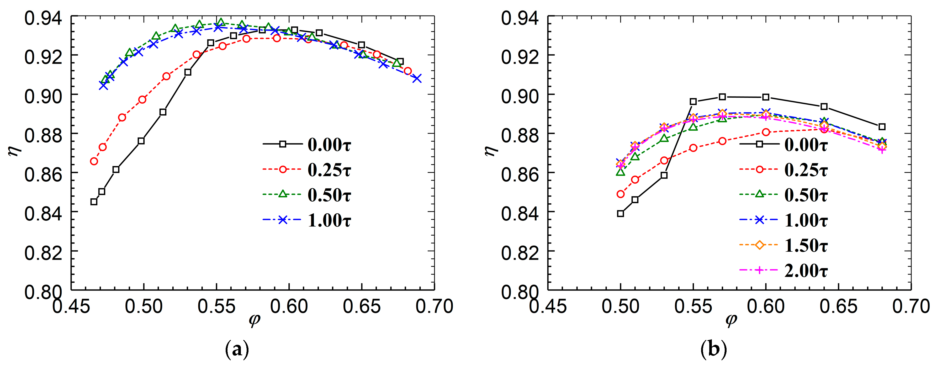
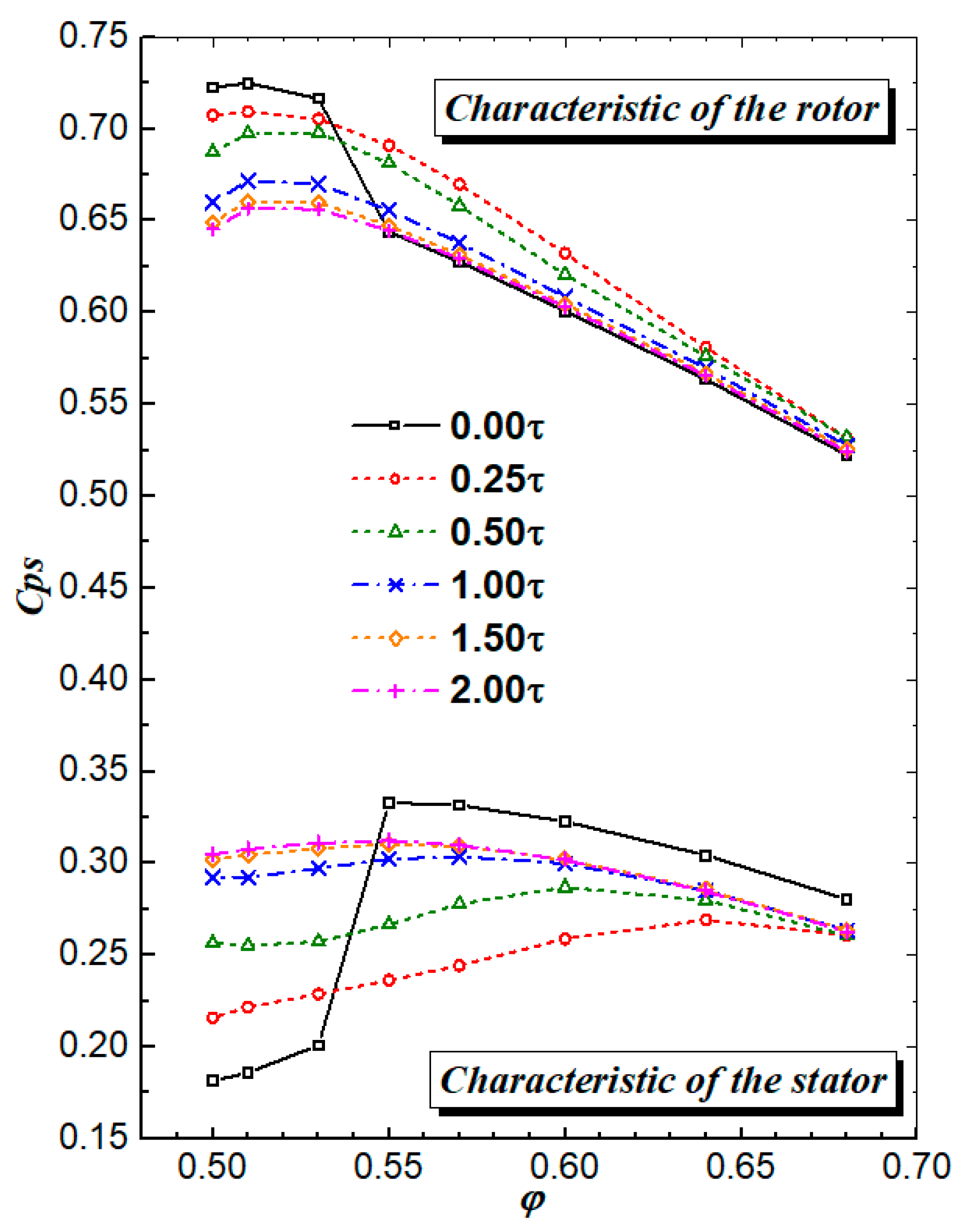
4.1. The Compressor Characteristics

Figure 3a and Figure 4a show the measured compressor static pressure-rise characteristics and compressor efficiency characteristics, respectively. For the compressor static pressure-rise coefficient, in brief, with the increase in the stator hub gap, at large mass flow conditions it decreases slightly at first, then drops obviously; at small mass flow conditions it increases rapidly at first, then drops slightly. Similar to the static pressure-rise coefficient, the compressor efficiency varies as the stator hub gap widens. Therefore, there should be an ideal stator hub gap that results in the optimal compressor performance; this ideal stator hub gap is between 0.50 τ and 1.00 τ.

Figure 3b and FIgure 4b show the simulated compressor static pressure-rise characteristics and compressor efficiency characteristics, respectively. Generally speaking, the CFD solver can predict the tendency of the variation in the compressor performance along with the stator hub gap, as described above. Moreover, when the stator is shrouded (i.e., 0.00 τ) the experimental results reveal that the compressor performance begins to drop rapidly at φ = 0.55. This phenomenon was also captured by the CFD results. Certainly, some differences still exist between the measured compressor performance and the CFD results, such as the changing amplitude when the stator hub gap increases and the value of the optimum stator hub gap. From the comparison, the simulated optimum stator hub gap seems to be a little higher than the measured results.

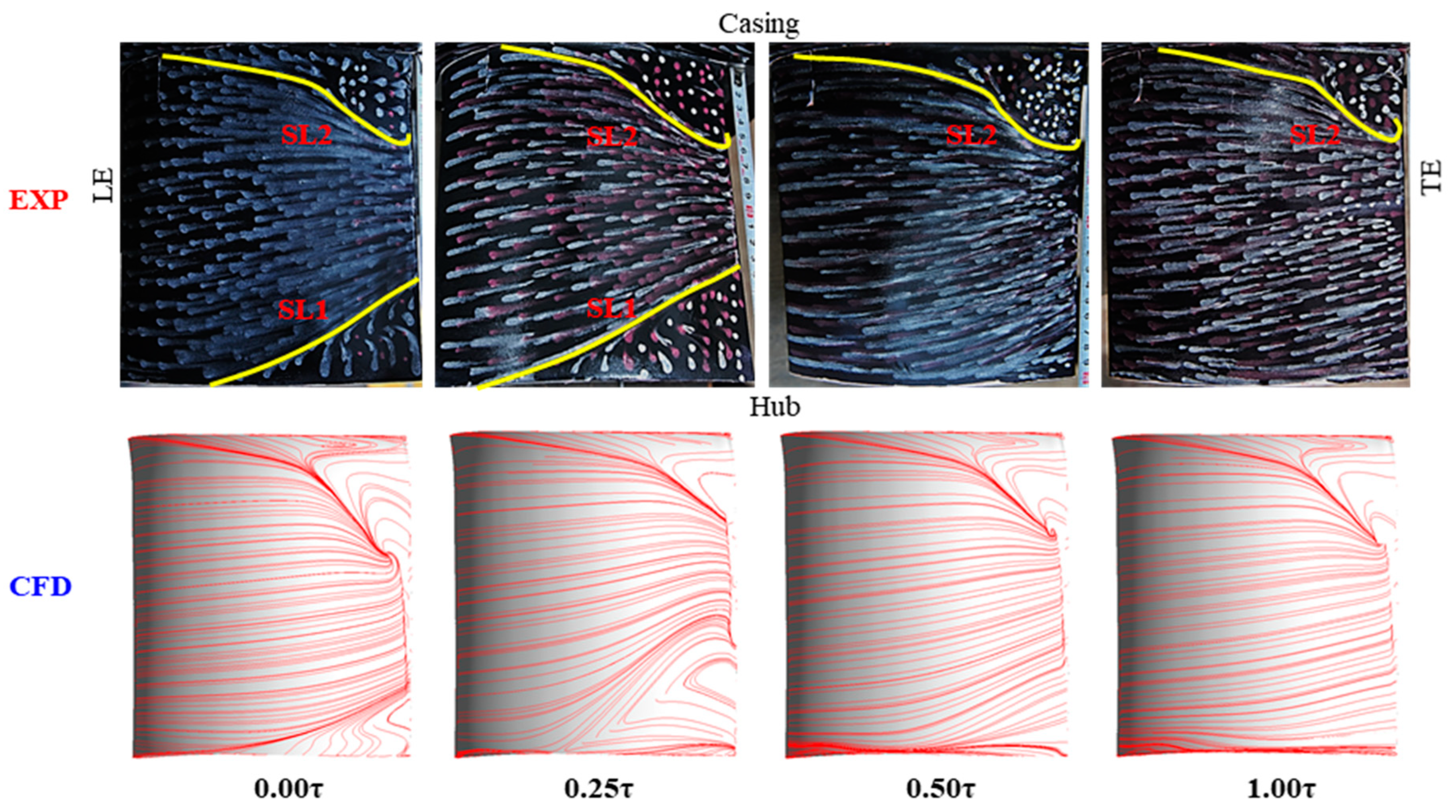
4.2. 3D Flow Structures inside the Stator Passage

As is known, the limiting streamline on the blade suction surface is usually used to reflect the 3D flow structures in the stator passage. Figure 5 shows the oil-flow visualization results as well as the simulated results for the DE condition. The mass flow coefficient for the DE condition is 0.6 in the experimental and CFD results. From the experimental results it can be seen that at 0.00, τ corner separation occurs at both the hub and the tip; at 0.25 τ, the two corner separations above still exist and the hub corner separation becomes stronger; at 0.50 τ and 1.00 τ, the hub corner separation disappears. These features were captured precisely by the CFD.

Figure 6 shows the oil-flow visualization results as well as the simulated results for the NS condition. The mass flow coefficient for the NS condition is 0.48 and 0.50 in the experimental and CFD results. From the experimental results, it can be seen that at 0.00 τ, the hub corner separation has already turned into a corner stall (combined with the oil-flow results on the hub) (see Liu et al. [14]); at 0.25 τ, the hub corner stall still exists, but from the flow field at the stator outlet shown below, it can be seen that the hub corner stall becomes a little weaker than at 0.00 τ; at 0.50 τ, the hub corner stall turns back into corner separation and the spanwise scale of the tip corner separation becomes larger; at 1.00τ, the hub corner separation seems to disappear and the spanwise scale of the tip corner separation becomes much larger. Obviously, at this condition, these features were captured precisely by the CFD again.

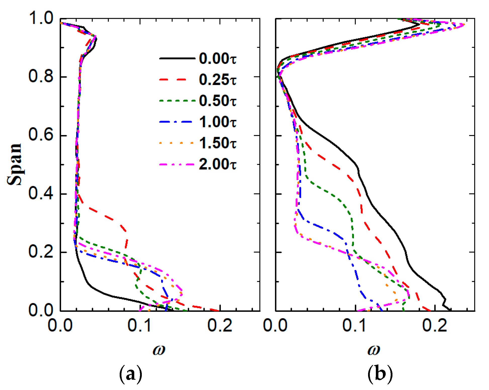
4.3. Flow Fields at the Stator Outlet

From above, it can be seen that the CFD solver can accurately predict the 3D flow structures inside the stator passage, but only the flow fields at the stator outlet can be used to quantitatively assess the effect of the separating flow or the leakage flow. The distributions of the normalized axial velocity at the stator outlet for the DE condition and the NS condition, respectively, are shown in Figure 7 and Figure 8. As the spanwise scale of the measured results is from 4% span to 97.5% span, two curves were added to the CFD results, which represent the lower and upper edge of the measured results.

According to the experimental findings under the DE condition, a low-velocity region is present at both ends of the wake when the stator is shrouded and corner separation occurs at both the hub and the tip; at 0.25 τ, the low-velocity region near the hub grows both spanwise and pitchwise; at 0.50 τ, it shrinks in the spanwise direction and slightly enlarges in the pitchwise direction; at 1.00 τ, the low-velocity region near the hub grows much larger in the pitchwise direction and somewhat smaller in the spanwise direction; in all cases, the low-velocity zone near the tip varies only a little. In contrast, the predicted scale of the low-velocity region near the hub by the CFD solver is a little different from the experimental results; for example, at 0.00 τ the scale is too small, and at 0.25 τ and 0.50 τ the scale is much bigger, but the predicted tendency of the variation along with the stator hub gap is right. This is also true for the prediction of the low-velocity region near the tip.

According to the experimental findings under the NS condition, the hub corner stall that occurs when the stator is shrouded results in a large low-velocity region at the hub corner; at 0.25 τ, this low-velocity region gets a little bit smaller in the pitchwise direction; at 0.50 τ, as the hub corner stall reverses to the corner separation, the low-velocity region gets considerably smaller; at 1.00 τ, the low-velocity zone close to the hub grows in the pitchwise direction while getting smaller in the spanwise direction; in addition, unlike the DE situation, when the stator hub gap rises from 0.25 blade height to 0.50 blade height, especially in the spanwise direction, the low-velocity zone near the tip corner becomes significantly greater. In comparison, the CFD solver can nearly predict both the scale and the tendency of the variation in the low-velocity region at the hub and the tip corner at this condition.

From above, it can be seen that the CFD solver used in this paper can almost reproduce the 3D separating flows inside the stator passage as the stator hub gap changes, not only in the tendency but also in the scale. Hence, it is feasible enough to be used to analyze the detailed flow mechanisms when the stator hub gap is induced.

5. Flow Mechanisms of the Effect of the Hub Clearance on the 3D Flows of the Stator

The low-energy flow inside the endwall boundary layer accumulates under the transverse pressure gradient from the blade pressure side to the suction side, and it separates under the streamwise unfavorable pressure gradient, as is well known, giving rise to the corner separation. When the stator hub gap is generated, a portion of the flow near the pressure side of the gap will pass through the gap and inject into the suction side, creating the leakage flow. This happens because of the pressure differential between the blade pressure side and the suction side. In other words, the leakage flow has the opposite effect on the endwall boundary layer compared to corner separation. On the one hand, the transverse component of the leakage flow momentum can prevent the transverse migration of the low-energy flow inside the endwall boundary layer. On the other hand, the streamwise component of the leakage flow momentum can help the flow to resist the streamwise adverse pressure gradient. Therefore, the interaction between the hub corner separation and the leakage flow is in fact the flow mechanism of the hub clearance’s influence on the stator’s three-dimensional flows.

5.1. Interaction between the Hub Corner Separation and the Leakage Flow

In this section, to clarify the interaction between hub corner separation and leakage flow, and the limiting streamline on the blade suction surface and the hub, the 3D streamline originates from the stator hub gap and the stator inlet boundary layer is depicted along with the stator outlet flow field (the axial velocity).

Figure 9 shows the 3D flow structures inside the stator passage at various stator hub gap configurations in the DE condition. At 0.00τ, only very weak corner separation occurs at the hub corner, so the 3D flow structure is relatively simple. The accumulation of the low-energy flow inside the endwall boundary layer towards the hub-SS corner is significant from the limiting streamline on the hub, and the slight separation of the accumulated low-energy flow is easy to see from the limiting streamline on the blade suction side.

At 0.25 τ, it is still clear that low-energy flow is accumulating within the endwall boundary layer at the hub–SS corner, and it also seems that the backflow on the blade suction side is stronger near the trailing edge. Backflow also occurs on the endwall, as can be observed from the limiting streamline on the hub, and no obvious leaking vortex can be detected from the 3D streamlines coming from the hub gap. This means that in this instance, the presence of the stator hub gap does not prevent the hub corner separation; rather, the leakage flow separates and causes the corner stall to occur. Therefore, in this case, the induced low-velocity region of the stator outlet is much larger than that at 0.00 τ.

At 0.50 τ, backflow on the blade suction side close to the trailing edge vanishes when the accumulation of low-energy flow inside the endwall boundary layer weakens significantly and approaches the hub–SS corner. Additionally, a clear separating line shows up on the hub where the boundary layer and leakage flow connect, and a line of attachment shows up on the blade suction surface, indicating the formation of the leakage vortex, which is also visible from the 3D streamlines coming from the hub gap. Therefore, the hub corner separation is removed in this instance and the leakage flow dominates the hub corner, resulting in a significantly smaller induced low-velocity area at the stator outlet than at 0.25 τ, but still bigger than at 0.00 τ.

At 1.00 τ, the concentration of low-energy flow within the endwall boundary layer towards the hub–SS corner weakens even further. The separating line on the hub moves further away from the blade suction side, the attachment line on the blade suction side indicated above vanishes, and the leaking vortex completely separates from the blade suction surface. Additionally, the leaking vortex grows stronger as seen by the 3D streamlines coming from the hub gap. As a result, in this situation, the induced low-velocity area changes from being smaller in one direction (spanwise) to being bigger in another (pitchwise).

At 1.50 τ and 2.00 τ, the feature of the 3D flow structures is similar to that at 1.00 τ, but the leakage vortex leaves further away from the blade suction side, so the accumulation of the low-energy flow inside the endwall boundary layer towards to the hub–SS corner becomes even weaker.

Figure 10 shows the 3D flow structures inside the stator passage at various stator hub gap configurations in the NS condition. At 0.00 τ, a focus point and backflows appear on the hub, which is the typical feature of the corner stall. From the 3D streamlines originating from the boundary layer, it also can be seen that the low-energy flow begins to roll up near the blade leading edge, and around the blade trailing edge it goes back to upstream. Hence, in this case, the hub corner stall happens; as a result, the induced low-velocity region at the stator outlet increases enormously.

At 0.25 τ, though a small hub gap is introduced, the backflows still exist, as can be seen from the limiting streamline on the hub and the 3D streamlines originating from the boundary layer. However, compared with the situation at 0.00 τ, the focus point on the hub becomes hard to see, and the place where the low-energy flow begins to roll up moves far away from the blade leading edge. That is to say, in this case, the hub corner stall still exists, but becomes weaker in contrast to that at 0.00 τ. Hence, the induced low-velocity region at the stator outlet becomes smaller.

At 0.50 τ, no limiting streamlining on the hub points upstream, and the concentration point on the hub totally disappears. The hub corner stall, therefore, vanishes. The hub corner separation still persists, though, and no concentrated leakage vortex arises, as can be seen from the limiting streamline on the blade suction side and the 3D streamlines coming from the hub gap and the boundary layer. Because of this, the hub corner is still primarily affected by the corner separation in this example, but when the corner stall is removed, the induced low-velocity zone at the stator outlet shrinks significantly.

At 1.00 τ, the separating line on the blade suction side (near the hub) is replaced by an attachment line, and the concentrated streamwise leakage vortex can be seen from the 3D streamlines originating from the hub gap. Hence, in this case, the hub corner separation disappears thoroughly and the leakage flow dominates the hub corner, so the induced low-velocity region at the stator outlet becomes even smaller. However, as the leakage flow is so close to the blade suction side, some interaction still exists between the leakage flow and the blade surface boundary layer. This is similar to that at the DE condition of 0.50 τ.

At 1.50 τ, the attachment line that was previously present on the blade suction side (near the hub) vanishes and the separation line on the hub moves further away from the blade suction side, i.e., the leakage vortex breaks away from the blade suction surface thoroughly. In addition, from the 3D streamlines originating from the hub gap, it can be seen that the leakage vortex becomes even stronger. Hence, in this case, the induced low-velocity region becomes even smaller. This is similar to the DE condition at 1.00 τ.

At 2.00 τ, the features of the 3D flow structures are similar to that at 1.50 τ, but the leakage vortex moves further away from the blade suction side, so the accumulation of the low-energy flow inside the endwall boundary layer towards to the hub–SS corner becomes even weaker. This is similar to the DE condition at 1.50 τ.

From above, the interaction between the leakage flow and the hub corner separation varies with the stator hub gap, and at different mass flow conditions the flow mechanism is also different. Generally speaking, when the stator is shrouded or a small hub gap is introduced, the hub corner will be dominated by the corner separation/stall, and when a big hub gap is introduced the hub corner will be dominated by the leakage flow. The specific situation depends on the momentum of the leakage flow.

5.2. Effect of the Hub Clearance on the Leakage Flow

As mentioned above, the transverse component of the leakage flow momentum can prevent the transverse migration of the low-energy flow inside the endwall boundary layer and the streamwise component of the leakage flow momentum can help the flow to resist the streamwise adverse pressure gradient. When the stator hub gap varies, the leakage flow velocity changes too. Figure 11 and Figure 12 show the distribution of the normalized streamwise component (tangent to the blade suction side) and the normalized normal component (perpendicular to the blade suction side) of leakage flow velocity at the suction side of the stator hub gap along the blade chord, respectively. Additionally, to make a comparison with the situation with no stator hub gap, in Figure 11, the normalized streamwise component of the velocity of the separating flow in the hub corner at 0.00 τ is also depicted.

It can be seen that in the DE condition, at most places the streamwise velocity of 0.00 τ is higher than that with a stator hub gap. The smaller the hub gap is, the lower the streamwise velocity will be, and so is the normal velocity. At 0.25 τ, the normal velocity of the leakage flow is too small to prevent the transverse migration of the low-energy flow inside the endwall boundary layer; instead, due to the very low streamwise velocity, when the flow in the boundary layer mixes with the leakage flow, the streamwise velocity of the flow in the boundary layer decreases sharply. Hence, under the effect of the streamwise adverse pressure gradient, the boundary layer separates. At 0.50 τ, both the streamwise velocity and the normal velocity of the leakage flow increases significantly. The momentum is the product of the mass flow and the velocity, and the mass flow is the product of the stator hub gap and the velocity; hence, the momentum of the leakage increases enormously. For example, the averaged normal component of the leakage flow velocity at 0.50 τ is 1.4 times of that at 0.25 τ; as a result, the averaged normal component of the leakage flow momentum at 0.50 τ is 4.0 times that at 0.25 τ. Hence, in this case, the transverse migration of the low-energy flow inside the endwall boundary layer is prevented effectively. Moreover, the averaged streamwise component of the leakage flow momentum at 0.50 τ is also about 4.0 times that at 0.25 τ; hence, after the mixing with the leakage flow, the streamwise momentum of the flow in the boundary layer is still able to resist the streamwise adverse pressure gradient. Therefore, in this case, no obvious backflow generates, and the hub corner is dominated by the leakage flow. When the stator hub gap increases continuously, both the streamwise velocity and the normal velocity of the leakage flow increase further, so the intensity of the leakage flow increases. However, as the stator hub gap exceeds 1.00 τ, the growing rates of both the streamwise velocity and the normal velocity of the leakage flow become very small.

In the NS condition, when the stator is cantilevered, both the streamwise velocity and the normal velocity of the leakage flow are almost the same as that of the DE condition. However, for the shrouded stator, as the hub corner separation turns into the corner stall, many backflows are generated in this condition. Hence, in most places, the streamwise velocity of 0.00 τ is negative. At 0.25 τ, though, the normal velocity of the leakage flow is still too small to prevent the transverse migration of the low-energy flow inside the endwall boundary layer; the mixing between the leakage flow and the separating flow can also increase the streamwise velocity of the flow in the boundary layer. Therefore, even though the hub corner stall still exists, the intensity of it becomes weaker. At 0.50 τ, as mentioned above, both the normal component and the streamwise component of the leakage flow momentum at 0.50 τ are about 4.0 times that at 0.25 τ. Even so, the normal velocity of the leakage flow is still not big enough to prevent the transverse migration of the low-energy flow inside the endwall boundary layer. However, after mixing with the leakage flow, the streamwise momentum of the flow in the boundary layer is big enough to resist the streamwise adverse pressure gradient. Hence, in this case, the hub corner stall turns back into corner separation. At 1.00 τ, both the streamwise velocity and the normal velocity of the leakage flow increase continuously, and so does the momentum of the leakage flow. This time, the hub corner separation completely vanishes, and the leakage flow predominates the hub corner because the normal velocity of the leakage flow is high enough to prohibit the transverse migration of the low-energy flow inside the endwall boundary layer. There is no need for further explanation, because the scenario is identical to the DE circumstance when the stator hub gap is continually increasing.

5.3. Discussion of the Optimum Hub Clearance

As mentioned above, the hub corner will separate or stall when the stator is shrouded or when a small hub gap is introduced; when the stator hub gap is sufficiently wide, the leakage flow will predominate the hub corner. Large flow blockage and flow loss are caused by hub corner stalls, and when leakage flow is too strong, the interaction of the leakage flow and the mainflow also causes significant flow blockage and loss. As a result, there typically is an ideal stator hub gap that results in the best compressor performance.

The circumferentially averaged normalized axial velocity at the stator outlet and the circumferentially averaged total pressure loss coefficient of the stator are shown in Figure 13 and Figure 14, respectively. In the DE condition, the flow loss and the flow blockage of the shrouded stator are the lowest. At 0.25 τ, the hub corner separation turns into a corner stall, so the spanwise range and the value of the flow blockage or flow loss increase abruptly; at 0.50 τ, the hub corner stall turns back to corner separation, so the spanwise range of the flow blockage or flow loss decreases significantly, but the value does not decrease; at 1.00 τ, the hub corner separation is replaced by the leakage flow, so the spanwise range of the flow blockage or flow loss decreases further, but the value becomes larger. As the stator hub gap increases continuously, both the spanwise range and the value of the flow loss begin to increase again, which is due to the strength of the leakage flow. In the NS condition, the situation is a little different from that in the DE condition. In this condition, the flow loss and the flow blockage of the shrouded stator are the highest. As the stator hub gap increases from 0.00 τ to 1.00 τ, both the spanwise range and the value of the flow blockage and flow loss decrease continuously. However, when the stator hub gap increases from 1.00 τ to 1.50 τ, the spanwise range and the value of the flow blockage decrease and the spanwise range of flow loss decreases, but the value increases, and when the stator hub gap increases from 1.50 τ to 2.00 τ, the spanwise range of the flow blockage and flow loss almost do not change and the value increases continuously.

The change in the cross section-averaged total pressure loss along with the stator hub gap is displayed in Figure 15 to provide a clear understanding of the impact of the stator hub gap on the stator’s flow loss. As can be observed, the ideal stator hub gap should be in the range of 0.50 τ to 1.00 τ, which is consistent with the study of compressor performance covered in Section 4.1. From the analysis above, this optimal stator hub gap only occurs when the induced leakage flow is similar to the corner separation, meaning that under situations of high mass flow rates, the induced leakage flow could reduce the corner separation, and under conditions of low mass flow rates, it could remove the corner stall, but does not result in additional mixing loss. The compressor performance will increase greatly under conditions of low mass flow rate and remain unchanged under situations of high mass flow rate.

As is known, both leakage flow and corner separation are promoted by the transverse pressure difference between the blade pressure side and the suction side. Hence, if without loss, the leakage flow is supposed to be comparable to the corner separation. However, in practice, due to the existence of the flow viscosity, loss will generate when leakage flow passes through the gap between the blade tip and the endwall. Therefore, for incompressible flow, the normal velocity can be calculated by Storer and Cumpsty [20]:

$$V_n=C_D\sqrt{\frac{2\times \left(p_{ps}-p_{ss}\right)}{\rho }}$$

(1)

Here, C_D is the discharge coefficient, and is dependent on the viscosity in the gap. Figure 16 shows the variation in C_D along with the stator hub gap. It can be seen that in the DE condition and in the NS condition the value of C_D is almost the same. When the stator hub gap is small, the viscosity in the gap is relatively high, so C_D is small. As the stator hub gap increases, the viscosity in the gap becomes relatively lower, so C_D increases. Until the stator hub gap is bigger than a certain value, the viscosity in the gap can be ignored and C_D almost does not change. Similarly, the streamwise velocity of the leakage flow is also dependent on the viscosity in the gap. Define the coefficient C_L as the ratio of the streamwise velocity at the suction side of the gap to the streamwise velocity at the pressure side of the gap. In Figure 16, the variation in C_L along with the stator hub gap is also displayed. It can be seen that the distribution of C_L is similar to that of C_D, i.e., it increases with the increment of the gap but almost does not change when the gap is bigger than a certain value. Hence, the optimum stator hub gap should be this critical value where the viscosity in the gap can be ignored.

Actually, through abundant data, Rains [21] has already proposed that the flow viscosity in the gap can only be disregarded when $R={\lambda }^{2}Reϵ>125$, where $Re$ is the Reynolds number based on the blade chord and the mainflow velocity near the hub, $ϵ$ is the ratio of the blade maximum thickness to the blade chord, and $\lambda$ is the ratio of the clearance size to the blade maximum thickness. The Reynolds number for the compressor under investigation is around $4\times {10}^5$, and the blade maximum thickness close to the hub is 10%. Hence, when the stator hub gap is 0.25 τ, the corresponding R equals 25; as a result, a lot of loss is generated as the flow passes through the gap and the leakage flow is much weaker than the corner separation; when the stator hub gap is 0.50τ, the corresponding R equals to 100, which is very close to the critical value, 125, so in this case the leakage flow is nearly comparable to the corner separation. By this analogy, the optimum stator hub gap should be 0.56τ, which coincides well with the results shown in Figure 15 and Figure 16. Hence, $R={\lambda }^{2}Reϵ=125$ could be a simple metric to choose the optimum stator hub gap.

To verify the metric above, some typical results from published papers are discussed here, as shown in Figure 17. Detailed information about the quoted results is summarized in

Table 1. Detail parameters of the quoted studies.

Researcher	Research Object	Methodology	Re	Blade Thickness/Chord
Gbadebo [9]	Cascade	CFD	4.8 × 105	5%
Wang [22]	Cascade	Experiment	3.2 × 105	8%
Chen [23]	Cascade	CFD	3 × 105	10%
George [7]	Low-speed compressor stator	CFD	1.1 × 105	10%
Sakulkaew [11]	High-speed compressor rotor	CFD	2 × 106	5%
Yang [24]	High-speed compressor stator	CFD	3 × 105	10%
McDougall [13]	Low-speed compressor rotor	Experiment	1.3 × 105	10%

. It can be seen that, for Wang’s results [22], in the P1 condition (where corner stall does not occur) when $R=125$, the loss reaches the local minimum and in the P2 condition (where corner stall happens) when $R=125$, the loss reaches the minimum, which coincides well with the results in this paper. In Chen’s [23] and George’s [7] results, when $R=125$, the loss is also near the minimum. In Gbadebo’s results [9], as the stator hub gap increases, the loss increases firstly, then decreases, and at last increases again; the evolution tendency of the loss with the variation in the gap is similar to the results in this paper, and when $R=125$ the loss does not reach but is very close to the local minimum. In Sakulkaew’s results [11], when $R=125$ the compressor efficiency is about the maximum. In Yang’s results [24], it is hard to judge if this metric is right as there are no investigated points between zero clearance and $R=125$, but for the results where $R>125$, the evolution tendency of the loss with the variation in the gap coincides well with the results in this paper. In McDoungall’s results [13], in both the DE and NS conditions the pressure-rise coefficient increases at first, then decreases as R increases, and the pressure-rise coefficient reaches the maximum around $R=125$. Hence, generally speaking, the metric proposed in this paper is feasible.

6. Effect of the Stator Hub Gap on the Stator Inlet Flow Fields and the Rotor Performance

When the stator hub gap is introduced, the 3D flow structures inside the stator passage change, and so do the flow blockage and flow loss, as discussed above. As the flow is subsonic, the variation in the flow blockage can also influence the upstream flow field. Hence, in this section, the rotor performance as well as the stator inlet flow fields will be discussed as the stator hub gap varies.

6.1. Variation of the Rotor Performance

Figure 18 depicts the stator and rotor’s static pressure-rise characteristics for various stator hub gap instances. As can be observed, the shrouded stator exhibits the largest static pressure rise under situations of big mass flow and the lowest static pressure rise under conditions of small mass flow. For stators with hub gaps, the larger the gap—whether under large mass flow conditions or small mass flow conditions—the greater the stator’s static pressure rise. The scenario is quite different for the rotor’s rise in static pressure, though.

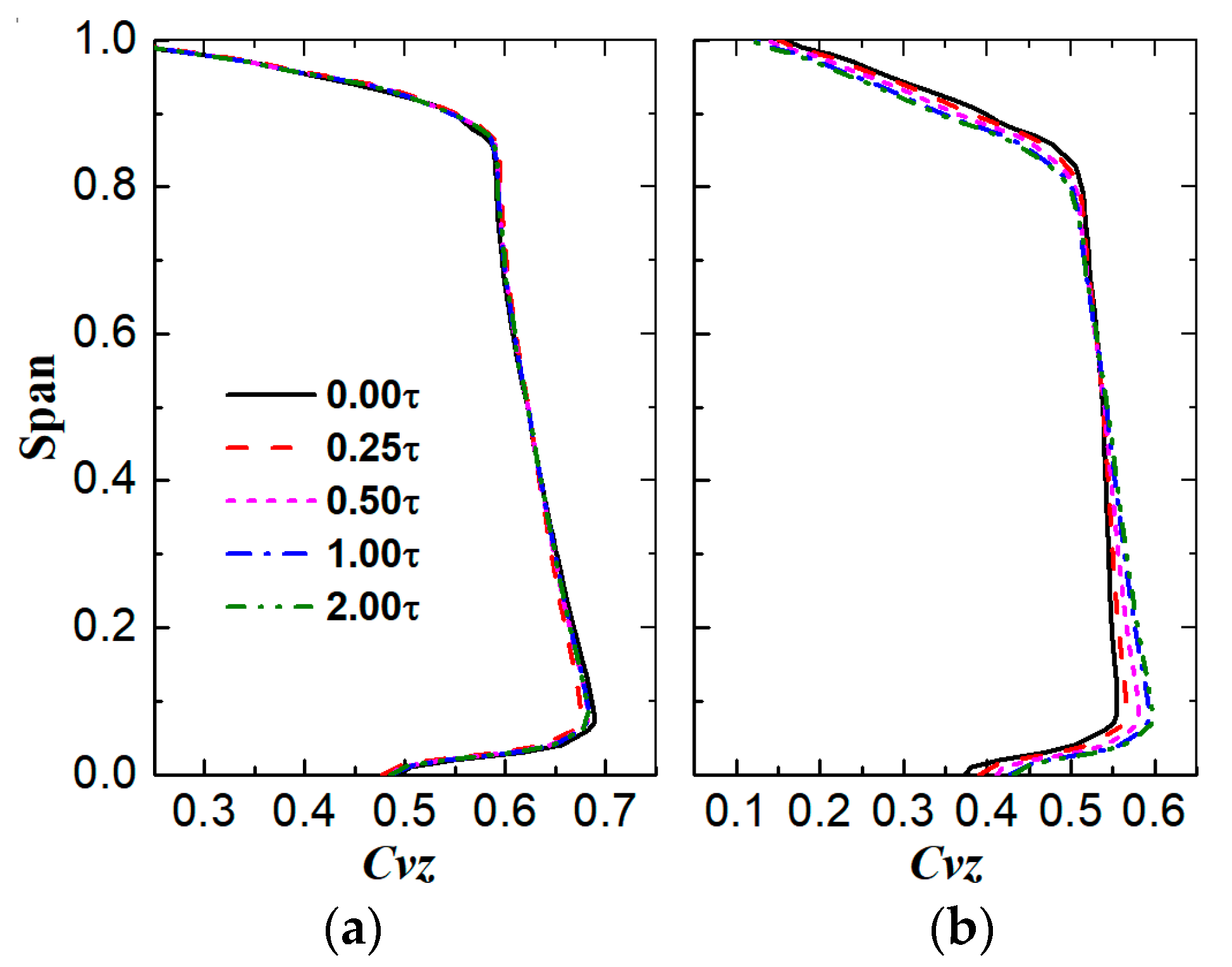
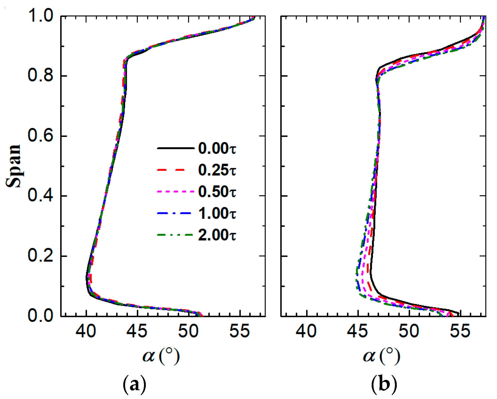
6.2. Variation in the Stator Inlet Flow Fields

According to Figure 13, the flow blockage at the hub of the shrouded stator is minimal under DE conditions; however, when a very tiny hub gap (0.25 τ) is applied, the blockage increases quickly, and the blockage becomes better as the stator hub gap grows continually. As shown in Figure 19a, when the flow near the stator hub is blocked, the flow capacity near the hub at the stator inlet also decreases, and the flow yaw angle in this region increases, as shown in Figure 20. This promotes more fluid to pass through the upper span of the rotor passage. The shrouded stator’s flow blockage is greatest under the NS condition, but when the stator hub gap widens, the blockage gradually diminishes, increasing the flow capacity close to the hub at the stator inlet. Less fluid flows across the upper span of the rotor passage as a result.

For a rotor, the work increases along with the blade height. In the DE condition, when a very small hub gap (0.25 τ) is introduced, more fluid passes through the upper span of the rotor passage, so the pressure rise in the rotor increases, and as the stator hub gap increases, less fluid passes through the upper span of the rotor passage, so the pressure rise in the rotor decreases. This is also true for the situation in the NS condition.

7. Conclusions and Prospects

The 3D flows inside the stator passage as well as the compressor’s performance are significantly impacted by the stator hub gap. The CFD approach was used to explore the flow mechanisms of the influence of the stator hub gap on the stator of a highly loaded low-speed axial compressor based on verification in contrast to the experimental results. The following conclusions can be made:

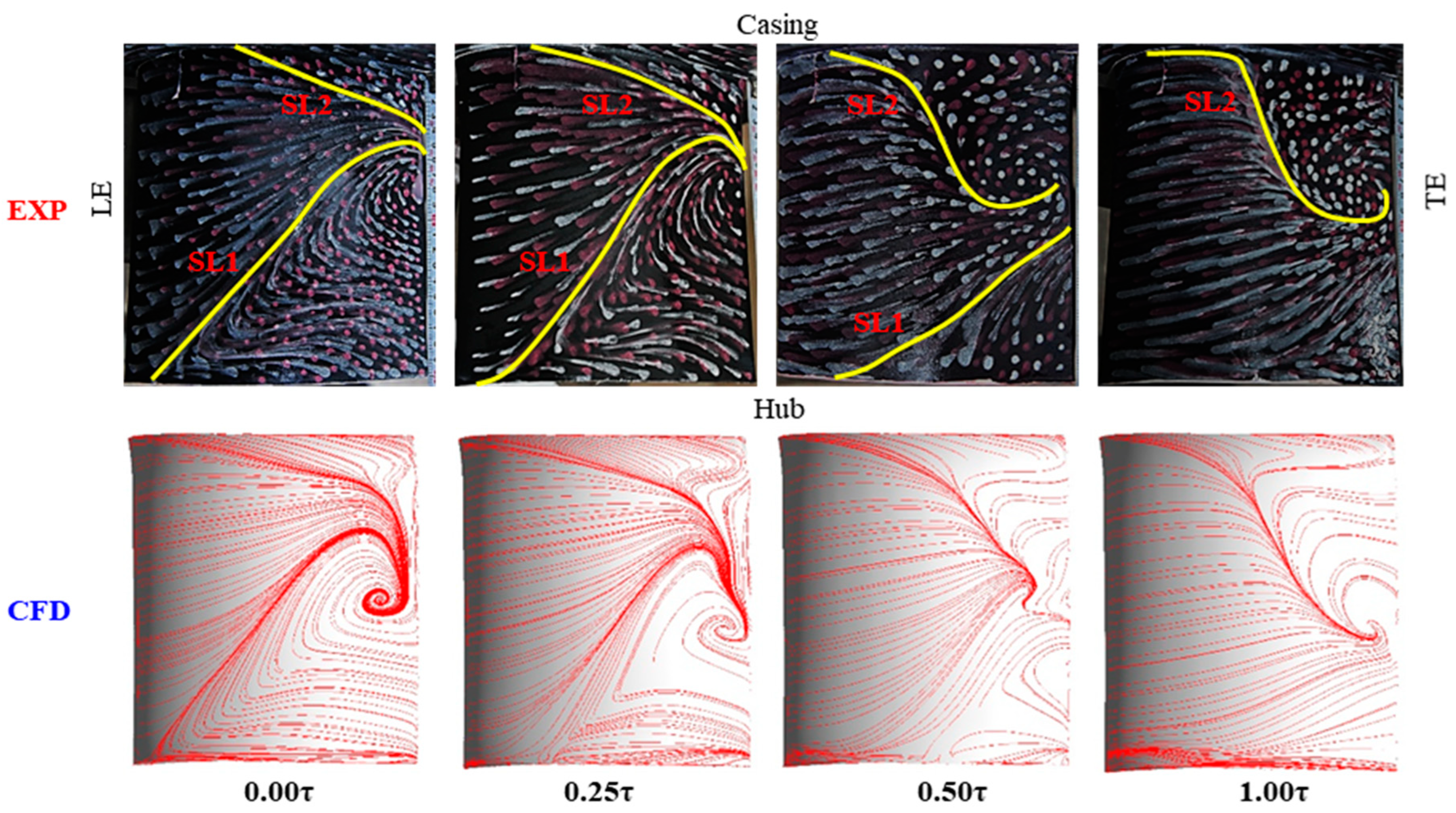
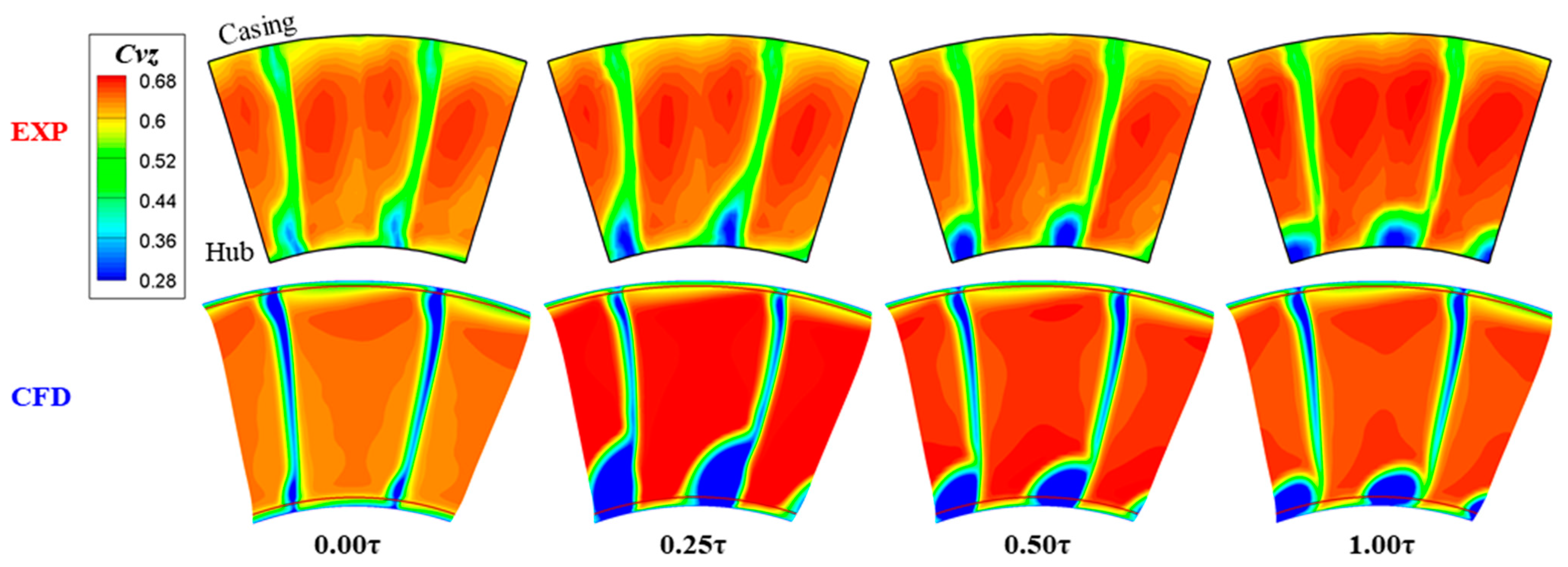
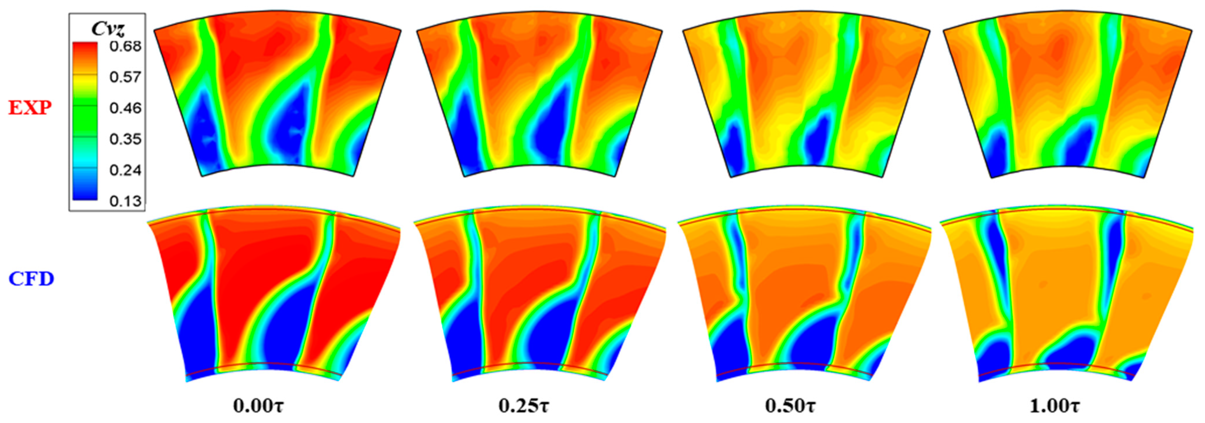
• The CFD solver and the corresponding setup used in this paper can almost reproduce the 3D separating flows inside the stator passage as the stator hub gap changes, not only in tendency but also in scale. Hence, it is feasible enough to be used to analyse the detailed flow mechanisms when the stator hub gap is induced.
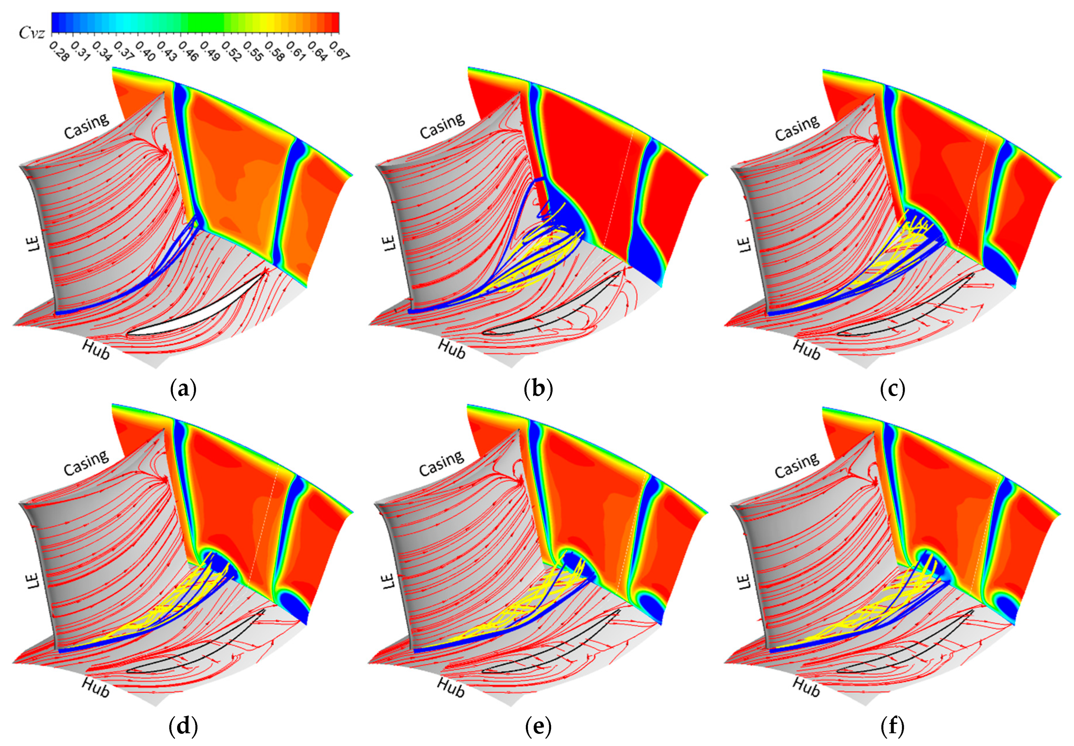
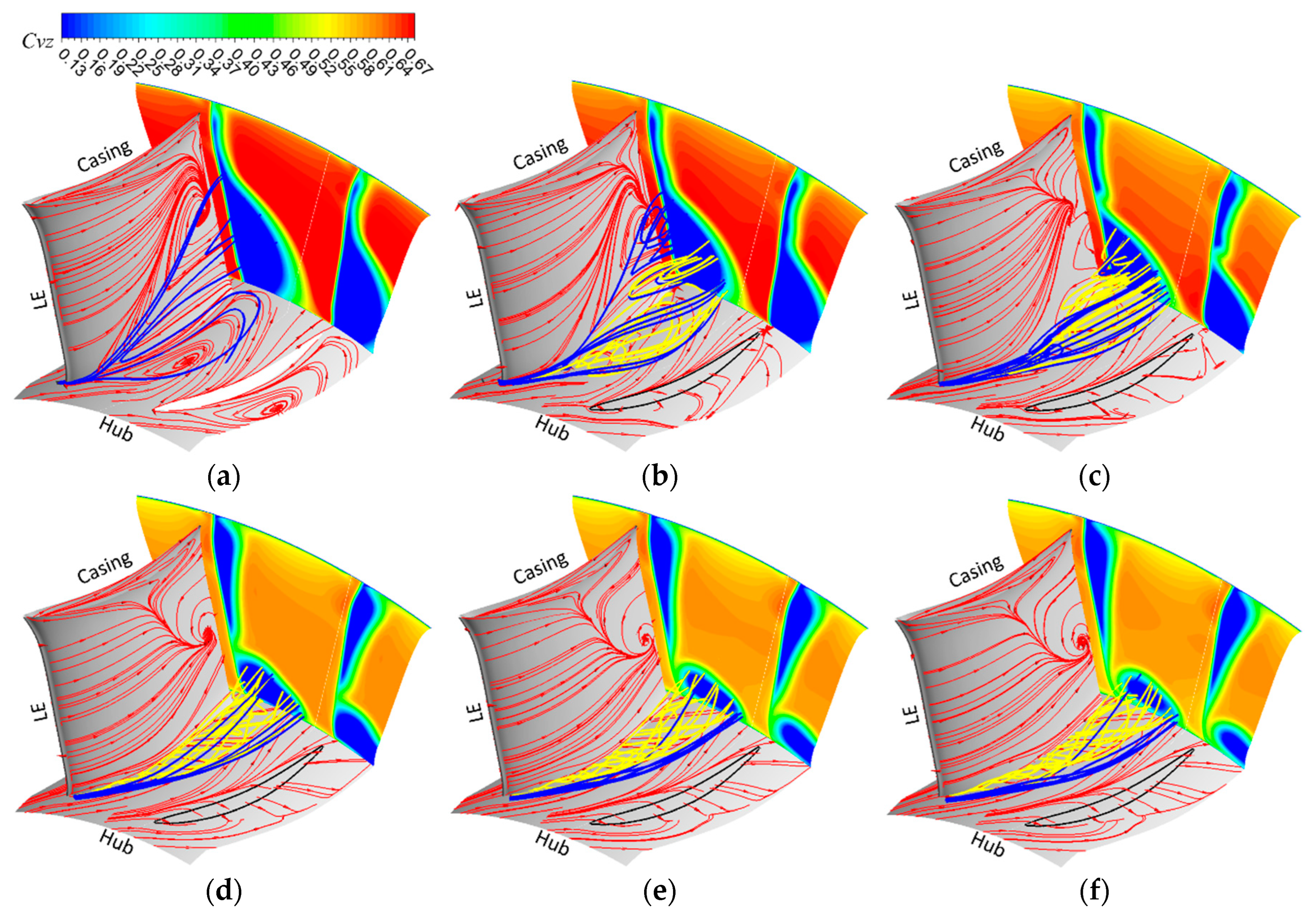
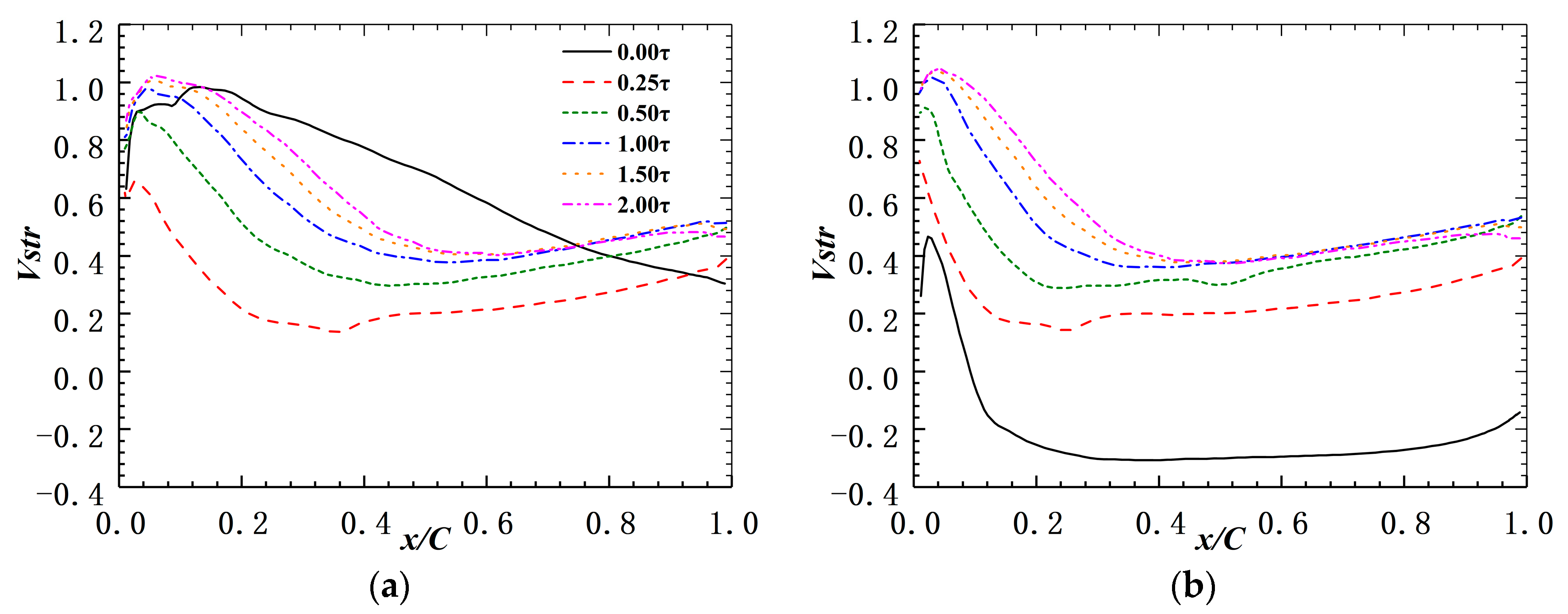
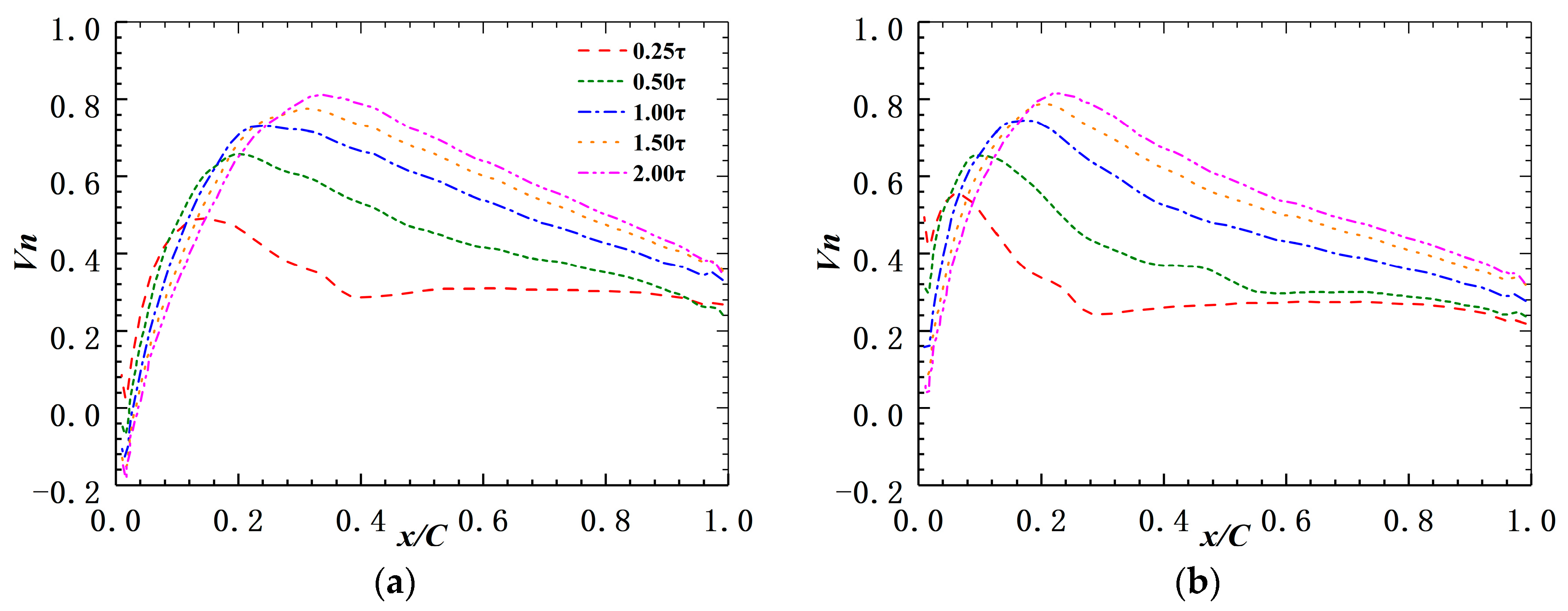
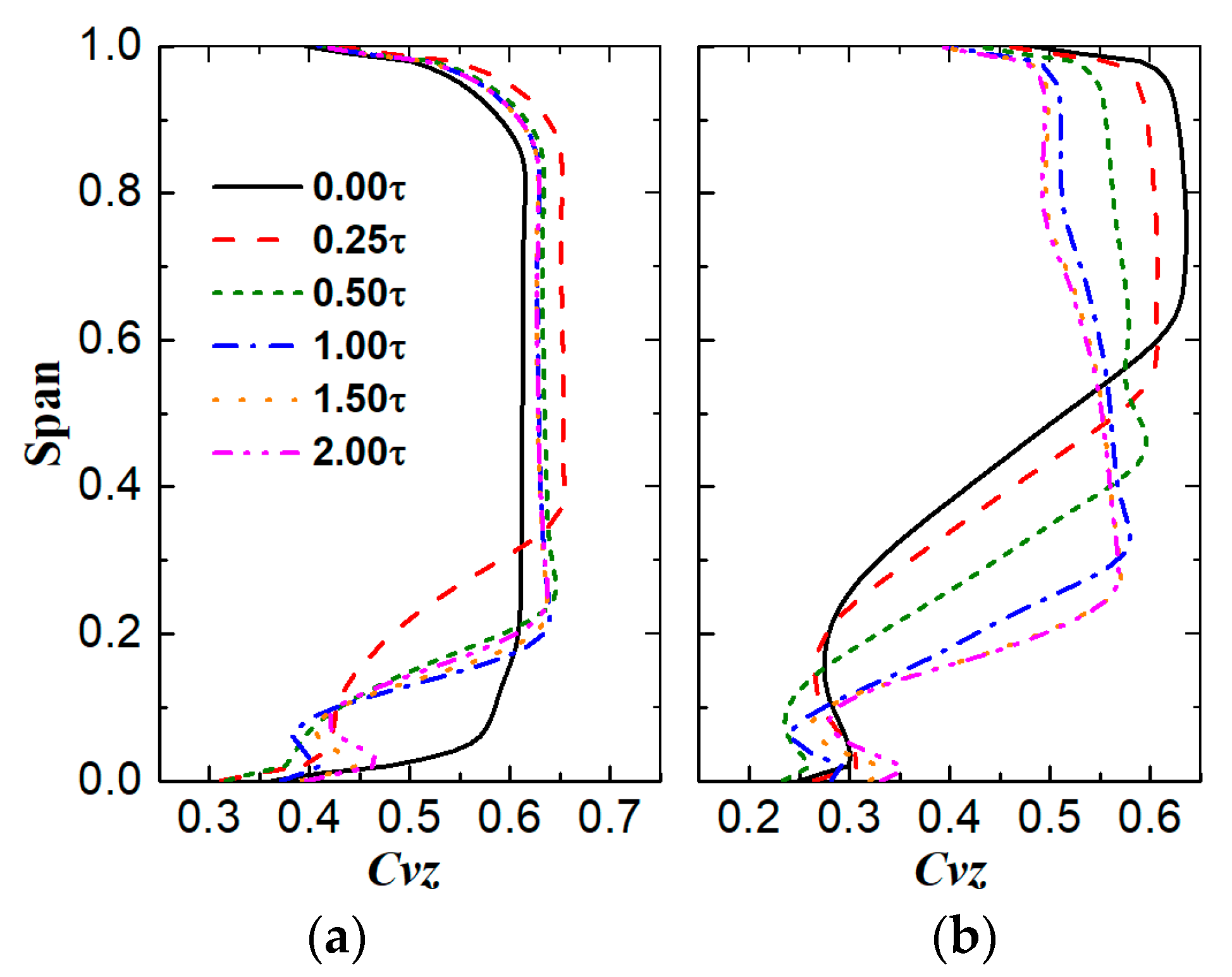
• The 3D flow structure inside the stator passage depends on the interaction between the leakage flow and the corner separation. Furthermore, it mainly depends on the velocity of the leakage flow. When the hub gap is too small, the velocity of the leakage flow is very low; in the DE condition, this becomes a low-energy flow, which will make the hub corner flow worse. However, in the NS condition, when a shrouded stator has a corner stall, this low-velocity leakage flow helps to improve the flow. The hub corner stall, or corner separation, gradually disappears as the stator hub gap widens, which increases the velocity of the leakage flow and, in turn, reduces flow loss and blockage. This trend continues until the stator hub gap increases to where the viscosity in the gap can be ignored. From then on, the velocity of the leakage flow will no longer increase apparently. Instead, as the gap increases, the leakage flow will increase, and the mixing between the leakage flow and the mainflow can also induce extra flow loss, and hence the compressor performance declines again.
• There exists an optimum stator hub gap where the leakage flow is comparable to the corner separation and the compressor performance is the best. This optimum gap, however, is equal to the gap where the viscosity in the gap can be ignored. Hence, using the method proposed by Rain, a simple metric was proposed to choose the optimum stator hub gap. By comparing our results with the results from published studies, this metric was proven to be feasible.
• Finally, it was also explained how the stator hub gap affected the stator inlet flow and rotor performance. It was demonstrated that the stator passage flow blockage can affect the upstream flow field. As a result, the performance of the rotor tends to vary in the opposite direction to that of the stator.

This paper numerically investigated the flow mechanisms of the effect of the hub gap on 3D flows inside the radial stacked stator of a highly loaded axial compressor stage, and a simple metric was proposed to determine the optimal stator hub gap. However, in actual axial compressors, 3D blade design technology is commonly used to improve endwall flow. Therefore, it is necessary to study the effect of the hub gap on the flow inside the stator under a condition in which the stator stacking axis is changed, and verify the method of choosing the optimal gap.

References

1. Dean, R.C. Secondary Flow in Axial Compressors; Massachusetts Institute of Technology: Cambridge, MA, USA, 1954. [Google Scholar]
2. Lakshminarayana, B.; Horlock, J.H. Tip-Clearance Flow and Losses for an Isolated Compressor Blade; Aeronautical Research Council London: London, UK, 1962. [Google Scholar]
3. Lakshminarayana, B.; Horlock, J.H. Leakage and Secondary Flows in Compressor Cascades; HM Stationery Office: Richmond, UK, 1965. [Google Scholar]
4. Lakshminarayana, B. Methods of Predicting the Tip Clearance Effects in Axial Flow Turbomachinery. J. Fluids Eng. 1970, 92, 467–480. [Google Scholar] [CrossRef]
5. Singh, U.K.; Ginder, R.B. The Effect of Hub Leakage Flow in a Transonic Compressor Stator. In Proceedings of the ASME 1998 International Gas Turbine and Aeroengine Congress and Exhibition, Stockholm, Sweden, 2–5 June 1998. [Google Scholar] [CrossRef]
6. Lee, C.; Song, J.; Lee, S.; Hong, D. Effect of a Gap Between Inner Casing and Stator Blade on Axial Compressor Performance. In Proceedings of the ASME Turbo Expo 2010: Power for Land, Sea, and Air, Glasgow, UK, 14–18 June 2010. [Google Scholar] [CrossRef]
7. George, K.K.; Agnimitra Sunkara, S.N.; George, J.T.; Joseph, M.; Pradeep, A.M.; Roy, B. Investigations on Stator Hub End Losses and its Control in an Axial Flow Compressor. In Proceedings of the ASME Turbo Expo 2014: Turbine Technical Conference and Exposition, Düsseldorf, Germany, 16–20 June 2014. [Google Scholar] [CrossRef]
8. Dong, Y.; Gallimore, S.J.; Hodson, H.P. Three-Dimensional Flows and Loss Reduction in Axial Compressors. J. Turbomach. 1987, 109, 354–361. [Google Scholar] [CrossRef]
9. Gbadebo, S.A.; Cumpsty, N.A.; Hynes, T.P. Interaction of Tip Clearance Flow and Three-Dimensional Separations in Axial Compressors. J. Turbomach. 2007, 129, 679–685. [Google Scholar] [CrossRef]
10. Peacock, R.E. A review of turbomachinery tip gap effects: Part 1: Cascades. Int. J. Heat Fluid Flow 1982, 3, 185–193. [Google Scholar] [CrossRef]
11. Sakulkaew, S.; Tan, C.S.; Donahoo, E.; Cornelius, C.; Montgomery, M. Compressor Efficiency Variation with Rotor Tip Gap from Vanishing to Large Clearance. J. Turbomach. 2013, 135, 031030. [Google Scholar] [CrossRef]
12. Wennerstrom, A.J. Experimental Study of a High-Throughflow Transonic Axial Compressor Stage. J. Eng. Gas Turbines Power 1984, 106, 552–560. [Google Scholar] [CrossRef]
13. McDougall, N.M. A Comparison Between the Design Point and Near-Stall Performance of an Axial Compressor. J. Turbomach. 1990, 112, 109–115. [Google Scholar] [CrossRef]
14. Liu, B.; Qiu, Y.; An, G.; Yu, X. Experimental Investigation of the Flow Mechanisms and the Performance Change of a Highly Loaded Axial Compressor Stage with/without Stator Hub Clearance. Appl. Sci. 2019, 9, 5134. [Google Scholar] [CrossRef]
15. Yu, X.J.; Liu, B.J. Research on three-dimensional blade designs in an ultra-highly loaded low-speed axial compressor stage: Design and numerical investigations. Adv. Mech. Eng. 2016, 8, 1–16. [Google Scholar] [CrossRef]
16. Liu, B.J.; An, G.F.; Yu, X.J. Assessment of Curvature Correction and Reattachment Modification into the Shear Stress Transport Model within the Subsonic Axial Compressor Simulations. Proc. Inst. Mech. Eng. Part A J. Power Energy 2015, 229, 910–927. [Google Scholar] [CrossRef]
17. Dener, C.; Hirsch, C. IGG—An Interactive 3D Surface Modelling and Grid Generation System. In Proceedings of the 30th Aerospace Sciences Meeting and Exhibit, Reno, NV, USA, 6–9 January 1992. [Google Scholar]
18. Menter, F.R. Two-equation eddy-viscosity turbulence models for engineering applications. AIAA J. 1994, 32, 1598–1605. [Google Scholar] [CrossRef]
19. Menter, F.R. Review of the shear-stress transport turbulence model experience from an industrial perspective. Int. J. Comput. Fluid Dyn. 2009, 23, 305–316. [Google Scholar] [CrossRef]
20. Storer, J.A.; Cumpsty, N.A. Tip Leakage Flow in Axial Compressors. J. Turbomach. 1991, 113, 252–259. [Google Scholar] [CrossRef]
21. Rains, D.A. Tip Clearance Flows in Axial Compressors and Pumps. Ph.D. Thesis, California Institute of Technology, Pasadena, CA, USA, 1954. [Google Scholar]
22. Wang, Z.; Geng, S.; Zhang, H. Influence of clearance variation on aerodynamic performance of a compressor stator cascade. Acta Aeronaut. Astronaut. Sin. 2016, 37, 3304–3316. [Google Scholar]
23. Chen, S.; Tsai, C.-R. The effect of tip clearance flow on compressor performance. In Proceedings of the 34th AIAA/ASME/SAE/ASEE Joint Propulsion Conference and Exhibit, Cleveland, OH, USA, 13–15 July 1998. [Google Scholar] [CrossRef]
24. Yang, C.; Lu, X.; Zhang, Y.; Zhao, S.; Zhu, J. Numerical Investigation of a Cantilevered Compressor Stator at Varying Clearance Sizes. In Proceedings of the ASME Turbo Expo 2015: Turbine Technical Conference and Exposition, Montreal, QC, Canada, 15–19 June 2015. [Google Scholar] [CrossRef]
Figure 1. The low-speed large-scale axial compressor test facility of Beihang University.
Energies 15 06993 g001
Figure 2. Numerical grids.
Energies 15 06993 g002
Figure 3. Characteristics of the compressor-stage static pressure-rise coefficient. (a) Experimental results; (b) CFD results.
Energies 15 06993 g003
Figure 4. Characteristics of compressor efficiency. (a) Experimental results; (b) CFD results.
Energies 15 06993 g004
Figure 5. Limiting streamlines on the stator suction surface in the DE condition.
Energies 15 06993 g005
Figure 6. Limiting streamlines on the stator suction surface in the NS condition.
Energies 15 06993 g006
Figure 7. Distribution of the normalized axial velocity of the stator outlet in the DE condition.
Energies 15 06993 g007
Figure 8. Distribution of the normalized axial velocity of the stator outlet in the NS condition.
Energies 15 06993 g008
Figure 9. Three-dimensional flow structures inside the stator passage in the DE condition. (a) 0.00 τ, (b) 0.25 τ, (c) 0.50 τ, (d) 1.00 τ, (e) 1.50 τ, (f) 2.00 τ.
Energies 15 06993 g009
Figure 10. Three-dimensional flow structures inside the stator passage in the NS condition. (a) 0.00 τ, (b) 0.25 τ, (c) 0.50 τ, (d) 1.00 τ, (e) 1.50 τ, (f) 2.00 τ.
Energies 15 06993 g010
Figure 11. Distribution of the normalized streamwise component of leakage flow velocity at the suction side of the stator hub gap along the blade chord. (a) In the DE condition; (b) in the NS condition.
Energies 15 06993 g011
Figure 12. Distribution of the normalized normal component of leakage flow velocity at the suction side of the stator hub gap along the blade chord. (a) In the DE condition; (b) in the NS condition.
Energies 15 06993 g012
Figure 13. Circumferentially averaged normalized axial velocity of stator outlet. (a) In the DE condition; (b) in the NS condition.
Energies 15 06993 g013
Figure 14. Circumferentially averaged total pressure loss coefficient of the stator. (a) In the DE condition; (b) in the NS condition.
Energies 15 06993 g014
Figure 15. Variation in the cross section-averaged total pressure loss along with the stator hub gap.
Energies 15 06993 g015
Figure 16. Variation in CD and CL along with the stator hub gap.
Energies 15 06993 g016
Figure 17. Published results about the optimum gap. (a) Variation in loss; (b) variation in efficiency; (c) variation in pressure rise.
Energies 15 06993 g017
Figure 18. Static pressure rise characteristics of the stator and the rotor.
Energies 15 06993 g018
Figure 19. Circumferentially averaged normalized axial velocity at stator inlet. (a) In the DE condition; (b) in the NS condition.
Energies 15 06993 g019
Figure 20. Circumferentially averaged flow yaw angle at stator inlet. (a) In the DE condition; (b) in the NS condition.
Energies 15 06993 g020