

Maximizing Efficient Power for an Irreversible Porous Medium Cycle with Nonlinear Variation of Working Fluid’s Specific Heat


Abstract
:1. Introduction
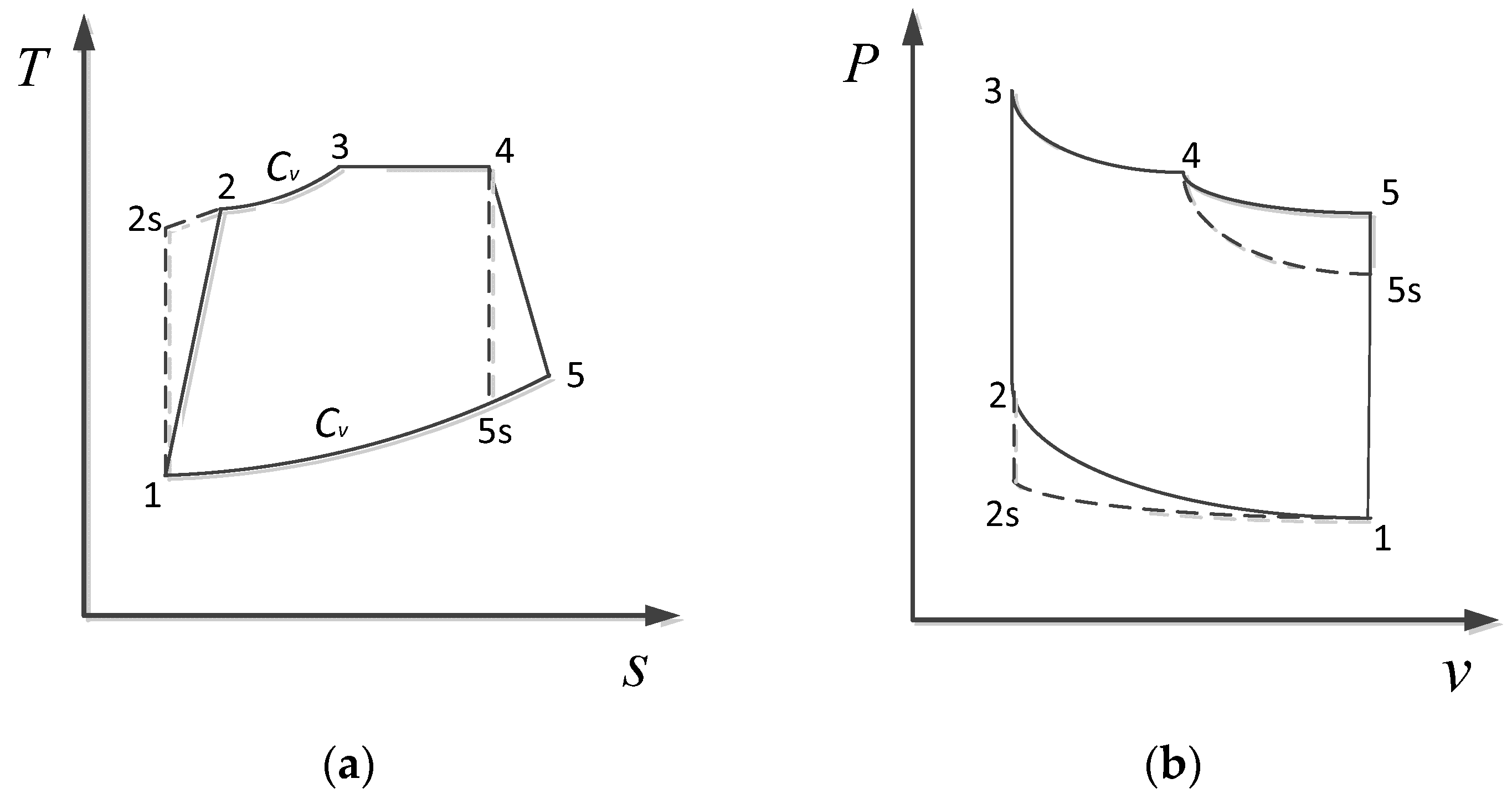
2. Model of PM
3. Efficient Power Maximization
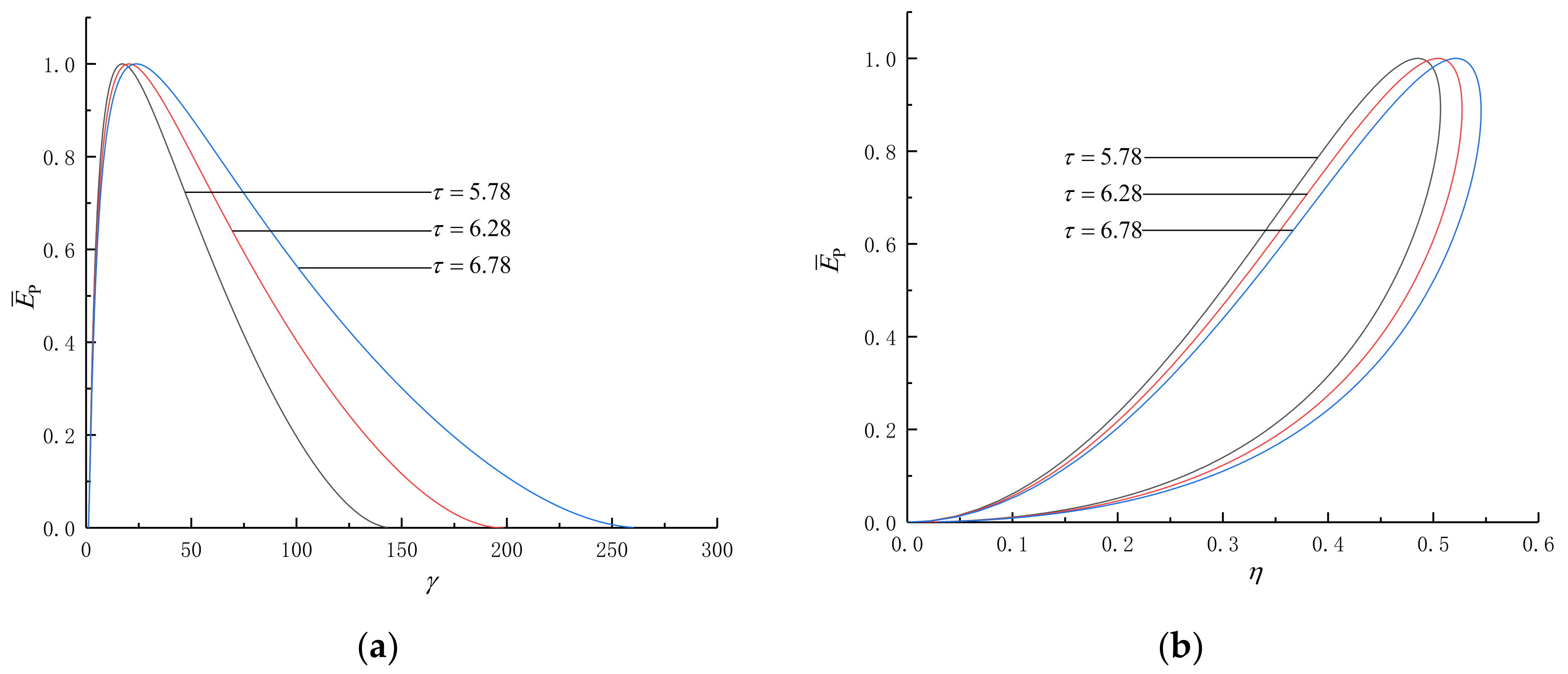
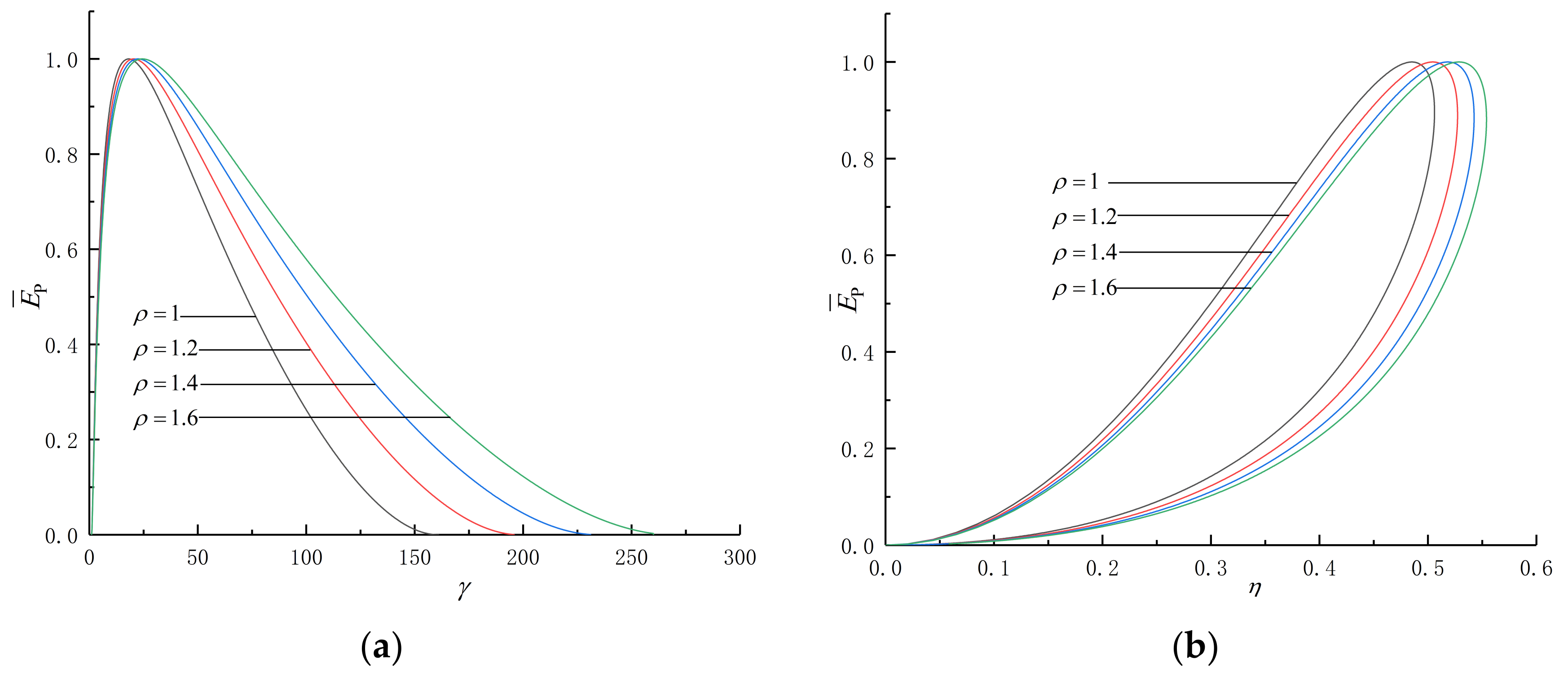
4. The Influences of SH Characteristics on Cycle Performance
5. Conclusions
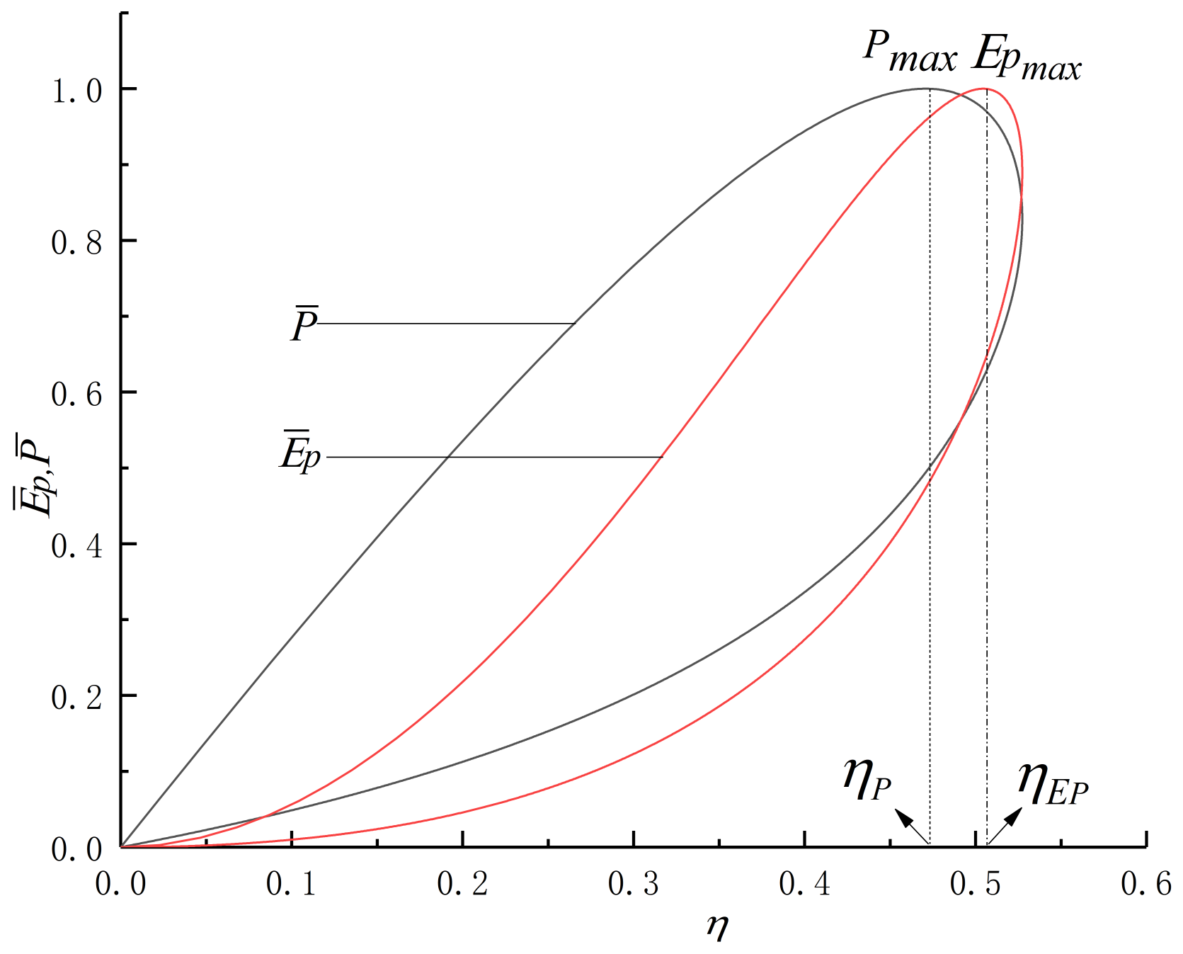
- The and curves of the cycle are a loop-shaped one and parabolic-like one, respectively. As and increase, both and increase. As and decrease and , , , and increase, both and decrease.
- By choosing the appropriate pre-expansion ratio, PM engine cycle can be converted to Otto engine cycle.
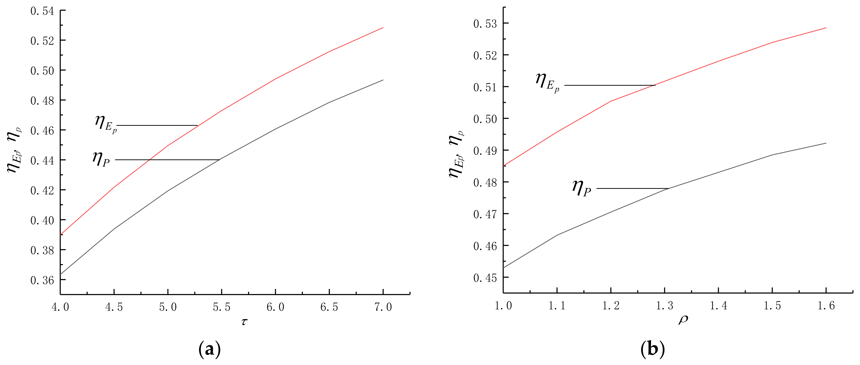
- Under specified conditions of different parameters, thermal efficiencies under the conditions of maximum efficient power and maximum power output are 50.45% and 47.05%, respectively. The latter is about 7.22% higher than the former.
- Efficient power objective function reflects the compromise between thermal efficiency and power output. The results of this paper can guide parameters selection of the actual heat engine.
Author Contributions
Funding
Institutional Review Board Statement
Informed Consent Statement
Data Availability Statement
Acknowledgments
Conflicts of Interest
Nomenclature
| Heat transfer loss coefficient () | |
| Specific heat at constant volume () | |
| Adiabatic index (-) | |
| Molar flow rate () | |
| Power output () | |
| Heat transfer rate () | |
| Gas constant () | |
| Temperature () | |
| Greek symbols | |
| Compression ratio (-) | |
| Thermal efficiency (-) | |
| Irreversible compression efficiency (-) | |
| Irreversible expansion efficiency (-) | |
| Friction loss coefficient () | |
| Pre-expansion ratio(-) | |
| Temperature ratio (-) | |
| Subscripts | |
| Input | |
| Heat leak | |
| Output | |
| Maximum value | |
| Max power output condition | |
| Max thermal efficiency condition | |
| Cycle state points | |
| Superscripts | |
| Dimensionless | |
| Abbreviations | |
| FL | Friction loss |
| FTT | Finite time thermodynamics |
| HTL | Heat transfer loss |
| IIL | Internal irreversibility loss |
| OF | Objective function |
| PM | Porous Medium |
| SH | Specific heats |
| WF | Working fluid |
Appendix A. Performance Indicators with Nonlinear Model of Variable SH
Appendix B. Performance Indicators with Model of Constant SH
Appendix C. Performance Indicators with Linear Model of Variable SH
References
- Andresen, B.; Berry, R.S.; Ondrechen, M.J.; Salamon, P. Thermodynamics for processes in finite time. Acc. Chem. Res. 1984, 17, 266–271. [Google Scholar] [CrossRef]
- Chen, L.G.; Wu, C.; Sun, F.R. Finite time thermodynamic optimization or entropy generation minimization of energy systems. J. Non-Equilib. Thermodyn. 1999, 24, 327–359. [Google Scholar]
- Andresen, B. Current trends in finite time thermodynamics. Angew. Chem. Int. Ed. 2011, 50, 2690–2704. [Google Scholar]
- Dumitrascu, G.; Feidt, M.; Popescu, A.; Grigorean, S. Endoreversible trigeneration cycle design based on finite physical dimensions thermodynamics. Energies 2019, 12, 3165. [Google Scholar]
- Abedinnezhad, S.; Ahmadi, M.H.; Pourkiaei, S.M.; Pourfayaz, F.; Mosavi, A.; Feidt, M.; Shamshirband, S. Thermodynamic assessment and multi-objective optimization of performance of irreversible Dual-Miller cycle. Energies 2019, 12, 4000. [Google Scholar] [CrossRef]
- Feidt, M.; Costea, M.; Feidt, R.; Danel, Q.; Périlhon, C. New criteria to characterize the waste heat recovery. Energies 2020, 13, 789. [Google Scholar] [CrossRef]
- Berry, R.S.; Salamon, P.; Andresen, B. How it all began. Entropy 2020, 22, 908. [Google Scholar] [CrossRef]
- Li, Z.X.; Cao, H.B.; Yang, H.X.; Guo, J.C. Comparative assessment of various low-dissipation combined models for three-terminal heat pump systems. Entropy 2021, 23, 513. [Google Scholar] [CrossRef] [PubMed]
- Yasunaga, T.; Fontaine, K.; Ikegami, Y. Performance evaluation concept for ocean thermal energy conversion toward standardization and intelligent design. Energies 2021, 14, 2336. [Google Scholar] [CrossRef]
- Sieniutycz, S. Complexity and Complex Chemo-Electric Systems; Elsevier: Amsterdam, The Netherlands, 2021. [Google Scholar]
- Andresen, B.; Salamon, P. Future perspectives of finite-time thermodynamics. Entropy 2022, 24, 690. [Google Scholar] [CrossRef]
- Ge, Y.L.; Chen, L.G.; Sun, F.R. Progress in finite time thermodynamic studies for internal combustion engine cycles. Entropy 2016, 18, 139. [Google Scholar] [CrossRef]
- Ahmadi, M.H.; Pourkiaei, S.M.; Ghazvini, M.; Pourfayaz, F. Thermodynamic assessment and optimization of performance of irreversible Atkinson cycle. Iran. J. Chem. Chem. Eng. 2020, 39, 267–280. [Google Scholar]
- Smith, Z.; Pal, P.S.; Deffner, S. Endoreversible Otto engines at maximal power. J. Non-Equilib. Thermodyn. 2020, 45, 305–310. [Google Scholar] [CrossRef]
- Shi, S.S.; Ge, Y.L.; Chen, L.G.; Feng, F.J. Four objective optimization of irreversible Atkinson cycle based on NSGA-II. Entropy 2020, 22, 1150. [Google Scholar] [CrossRef]
- Levario-Medina, S.; Valencia-Ortega, G.; Barranco-Jimenez, M.A. Energetic optimization considering a generalization of the ecological criterion in traditional simple-cycle and combined cycle power plants. J. Non-Equilib. Thermodyn. 2020, 45, 269–290. [Google Scholar]
- Ding, Z.M.; Ge, Y.L.; Chen, L.G.; Feng, H.J.; Xia, S.J. Optimal performance regions of Feynman’s ratchet engine with different optimization criteria. J. Non-Equilib. Thermodyn. 2020, 45, 191–207. [Google Scholar] [CrossRef]
- Tang, C.Q.; Chen, L.G.; Feng, H.J.; Wang, W.H.; Ge, Y.L. Power optimization of a modified closed binary Brayton cycle with two isothermal heating processes and coupled to variable-temperature reservoirs. Energies 2020, 13, 3212. [Google Scholar] [CrossRef]
- Liu, X.W.; Chen, L.G.; Ge, Y.L.; Feng, H.J.; Wu, F.; Lorenzini, G. Exergy-based ecological optimization of an irreversible quantum Carnot heat pump with spin-1/2 systems. J. Non-Equilib. Thermodyn. 2021, 46, 61–76. [Google Scholar] [CrossRef]
- Lai, H.Y.; Li, Y.T.; Chan, Y.H. Efficiency enhancement on hybrid power system composed of irreversible solid oxide fuel cell and Stirling engine by finite time thermodynamics. Energies 2021, 14, 1037. [Google Scholar] [CrossRef]
- Dumitrașcu, G.; Feidt, M.; Grigorean, S. Finite physical dimensions thermodynamics analysis and design of closed irreversible cycles. Energies 2021, 14, 3416. [Google Scholar] [CrossRef]
- Shi, S.S.; Ge, Y.L.; Chen, L.G.; Feng, F.J. Performance optimizations with single-, bi-, tri- and quadru-objective for irreversible Atkinson cycle with nonlinear variation of working fluid’s specific heat. Energies 2021, 14, 4175. [Google Scholar] [CrossRef]
- Paul, R.; Hoffmann, K.H. A class of reduced-order regenerator models. Energies 2021, 14, 7295. [Google Scholar] [CrossRef]
- Qiu, S.S.; Ding, Z.M.; Chen, L.G.; Ge, Y.L. Performance optimization of thermionic refrigerators based on van der Waals heterostructures. Sci. China Technol. Sci. 2021, 64, 1007–1016. [Google Scholar] [CrossRef]
- Badescu, V. Self-driven reverse thermal engines under monotonous and oscillatory optimal operation. J. Non-Equilib. Thermodyn. 2021, 46, 291–319. [Google Scholar] [CrossRef]
- Qi, C.Z.; Ding, Z.M.; Chen, L.G.; Ge, Y.L.; Feng, H.J. Modelling of irreversible two-stage combined thermal Brownian refrigerators and their optimal performance. J. Non-Equilib. Thermodyn. 2021, 46, 175–189. [Google Scholar] [CrossRef]
- Valencia-Ortega, G.; Levario-Medina, S.; Barranco-Jiménez, M.A. The role of internal irreversibilities in the performance and stability of power plant models working at maximum ϵ-ecological function. J. Non-Equilib. Thermodyn. 2021, 46, 413–429. [Google Scholar] [CrossRef]
- Qiu, S.S.; Ding, Z.M.; Chen, L.G.; Ge, Y.L. Performance optimization of three-terminal energy selective electron generators. Sci. China Technol. Sci. 2021, 64, 1641–1652. [Google Scholar] [CrossRef]
- He, J.H.; Chen, L.G.; Ge, Y.L.; Shi, S.S.; Li, F. Multi-objective optimization of an irreversible single resonance energy-selective electronic heat engine. Energies 2022, 24, 1074. [Google Scholar]
- Chen, Y.R. Maximum profit configurations of commercial engines. Entropy 2011, 13, 1137–1151. [Google Scholar] [CrossRef]
- Ebrahimi, R. A new design method for maximizing the work output of cycles in reciprocating internal combustion engines. Energy Convers. Manag. 2018, 172, 164–172. [Google Scholar] [CrossRef]
- Boikov, S.Y.; Andresen, B.; Akhremenkov, A.A.; Tsirlin, A.M. Evaluation of irreversibility and optimal organization of an integrated multi-stream heat exchange system. J. Non-Equilib. Thermodyn. 2020, 45, 155–171. [Google Scholar] [CrossRef]
- Chen, L.G.; Ma, K.; Feng, H.J.; Ge, Y.L. Optimal configuration of a gas expansion process in a piston-type cylinder with generalized convective heat transfer law. Energies 2020, 13, 3229. [Google Scholar] [CrossRef]
- Scheunert, M.; Masser, R.; Khodja, A.; Paul, R.; Schwalbe, K.; Fischer, A.; Hoffmann, K.H. Power-optimized sinusoidal piston motion and its performance gain for an Alpha-type Stirling engine with limited regeneration. Energies 2020, 13, 4564. [Google Scholar] [CrossRef]
- Masser, R.; Hoffmann, K.H. Optimal control for a hydraulic recuperation system using endoreversible thermodynamics. Appl. Sci. 2021, 11, 5001. [Google Scholar] [CrossRef]
- Paul, R.; Hoffmann, K.H. Cyclic control optimization algorithm for Stirling engines. Symmetry 2021, 13, 873. [Google Scholar] [CrossRef]
- Khodja, A.; Paul, R.; Fischer, A.; Hoffmann, K.H. Optimized cooling power of a Vuilleumier refrigerator with limited regeneration. Energies 2021, 14, 8376. [Google Scholar] [CrossRef]
- Badescu, V. Maximum work rate extractable from energy fluxes. J. Non-Equilib. Thermodyn. 2022, 47, 77–93. [Google Scholar] [CrossRef]
- Paul, R.; Hoffmann, K.H. Optimizing the piston paths of Stirling cycle cryocoolers. J. Non-Equilib. Thermodyn. 2022, 47, 195–203. [Google Scholar] [CrossRef]
- Li, P.L.; Chen, L.G.; Xia, S.J.; Kong, R.; Ge, Y.L. Total entropy generation rate minimization configuration of a membrane reactor of methanol synthesis via carbon dioxide hydrogenation. Sci. China Technol. Sci. 2022, 65, 657–678. [Google Scholar] [CrossRef]
- Fischer, A.; Khodja, A.; Paul, R.; Hoffmann, K.H. Heat-only-driven Vuilleumier refrigeration. Appl. Sci. 2022, 12, 1775. [Google Scholar] [CrossRef]
- Li, J.; Chen, L.G. Optimal configuration of finite source heat engine cycle for maximum output work with complex heat transfer law. J. Non-Equilib. Thermodyn. [CrossRef]
- Klein, S.A. An explanation for observed compression ratios in international combustion engines. J. Eng. Gas Turbines Power 1991, 113, 511–513. [Google Scholar] [CrossRef]
- Ghatak, A.; Chakraborty, S. Effect of external irreversibilities and variable thermal properties of working fluid on thermal performance of a Dual internal combustion engine cycle. J. Mech. Energy 2007, 58, 1–12. [Google Scholar]
- Abu-Nada, E.; Al-Hinti, I.; Al-Sarkhi, A.; Akash, B. Thermodynamic modeling of spark-ignition engine: Effect of temperature dependent specific heats. Int. Commun. Heat Mass Transfer 2006, 33, 1264–1272. [Google Scholar] [CrossRef]
- Angulo-Brown, F.; Rocha-Martinez, J.A.; Navarrete-Gonzalez, T.D. A non-endoreversible Otto cycle model: Improving power output and efficiency. J. Phys. D Appl. Phys. 1996, 29, 80–83. [Google Scholar] [CrossRef]
- Angulo-Brown, F.; Fernandez, B.J.; Diaz-Pico, C.A. Compression ratio of an optimized Otto-cycle model. Eur. J. Phys. 1994, 15, 38. [Google Scholar] [CrossRef]
- Chen, L.G.; Zen, F.M.; Sun, F.R. Heat transfer effects on the network output and power as function of efficiency for air standard Diesel cycle. Energy 1996, 21, 1201–1205. [Google Scholar] [CrossRef]
- Angulo-Brown, F. An ecological optimization criterion for finite-time heat engines. J. Appl. Phys. 1991, 69, 7465–7469. [Google Scholar] [CrossRef]
- Sahin, B.; Kodal, A.; Yavuz, H. Efficiency of a Joule-Brayton engine at maximum power density. J. Phys. D Appl. Phys. 1995, 28, 1309. [Google Scholar] [CrossRef]
- Yan, Z.J. η and P of a Carnot engine at maximum ηP. Chin. J. Nat. 1984, 7, 475. (In Chinese) [Google Scholar]
- Gonca, G.; Genc, I. Thermoecology-based performance simulation of a Gas-Mercury-Steam power generation system (GMSPGS). Energy Convers. Manag. 2019, 189, 91–104. [Google Scholar] [CrossRef]
- Gonca, G.; Genc, I. Performance simulation of a double-reheat Rankine cycle mercury turbine system based on exergy. Int. J. Exergy 2019, 30, 392–403. [Google Scholar] [CrossRef]
- Chen, L.G.; Tang, C.Q.; Feng, H.J.; Ge, Y.L. Power, efficiency, power density and ecological function optimizations for an irreversible modified closed variable-temperature reservoir regenerative Brayton cycle with one isothermal heating process. Energies 2020, 13, 5133. [Google Scholar] [CrossRef]
- Diskin, D.; Tartakovsky, L. Efficiency at maximum power of the low-dissipation hybrid electrochemical–otto cycle. Energies 2020, 13, 3961. [Google Scholar] [CrossRef]
- Wang, R.B.; Chen, L.G.; Ge, Y.L.; Feng, H.J. Optimizing power and thermal efficiency of an irreversible variable-temperature heat reservoir Lenoir cycle. Appl. Sci. 2021, 11, 7171. [Google Scholar] [CrossRef]
- Gonca, G.; Hocaoglu M, F. Exergy-based performance analysis and evaluation of a dual-diesel cycle engine. Therm. Sci. 2021, 25, 3675–3685. [Google Scholar] [CrossRef]
- Gonca, G.; Sahin, B. Performance investigation and evaluation of an engine operating on a modified dual cycle. Int. J. Energy Res. 2022, 46, 2454–2466. [Google Scholar] [CrossRef]
- Paul, R.; Khodja, A.; Fischer, A.; Masser, R.; Hoffmann, K.H. Power-optimal control of a Stirling engine’s frictional piston motion. Entropy 2022, 24, 362. [Google Scholar] [CrossRef]
- Bellos, E.; Lykas, P.; Tzivanidis, C. Investigation of a solar-driven organic Rankine cycle with reheating. Appl. Sci. 2022, 12, 2322. [Google Scholar] [CrossRef]
- Yilmaz, T. A new performance criterion for heat engines: Efficient power. J. Energy Inst. 2006, 79, 38–41. [Google Scholar] [CrossRef]
- Atmaca, M.; Gümüş, M.; Demir, A. Comparative thermodynamic analysis of dual cycle under alternative conditions. Therm. Sci. 2011, 15, 953–960. [Google Scholar] [CrossRef]
- Reyes-Ramírez, I.; Barranco-Jiménez, M.A.; Rojas-Pacheco, A.; Guzmán-Vargas, L. Global stability analysis of a Curzon–Ahlborn heat engine under different regimes of performance. Entropy 2014, 16, 5796–5809. [Google Scholar] [CrossRef]
- Kumar, R.; Kaushik, S.C.; Kumar, R. Performance optimization of Brayton heat engine at maximum efficient power using temperature dependent specific heat of working fluid. J. Therm. Eng. 2015, 1, 345–354. [Google Scholar] [CrossRef]
- Gonca, G. Performance analysis of an Atkinson cycle engine under effective power and effective power density condition. Acta Phys. Polon. 2017, 132, 1306–1313. [Google Scholar] [CrossRef]
- Gonca, G.; Hocaoglu, M.F. Performance Analysis and Simulation of a Diesel-Miller Cycle (DiMC) Engine. Arabian J. Sci. Eng. 2019, 44, 5811–5824. [Google Scholar] [CrossRef]
- Gonca, G.; Sahin, B. Performance analysis of a novel eco-friendly internal combustion engine cycle. Int. J. Energy Res. 2019, 43, 5897–5911. [Google Scholar] [CrossRef]
- Gonca, G.; Sahin, B.; Genc, I. Investigation of maximum performance characteristics of seven-process cycle engine. Int. J. Exergy 2022, 37, 302–312. [Google Scholar] [CrossRef]
- Nilavarasi, K.; Ponmurugan, M. Optimized efficiency at maximum figure of merit and efficient power of power law dissipative Carnot like heat engines. J. Stat. Mech. Theory Exp. 2021, 4, 043208. [Google Scholar] [CrossRef]
- Ferrenberg, A.J. The Single Cylinder Regenerated Internal Combustion Engine. In Proceedings of the Earthmoving Industry Conference & Exposition, Canoga Park, CA, USA, 1 April 1990. [Google Scholar] [CrossRef]
- Howell, J.R.; Hall, M.J.; Ellzey, J.L. Combustion of hydrocarbon fuels within porous inert media. Prog. Energy Combust. Sci. 1996, 22, 121–145. [Google Scholar] [CrossRef]
- Durst, F.; Weclas, M. A new type of internal combustion engine based on the porous-medium combustion technique. Proc. Inst. Mech. Eng. D J. Automob. Eng. 2001, 215, 63–81. [Google Scholar] [CrossRef]
- Liu, H.S.; Xie, M.Z.; Chen, S. Thermodynamic analysis of ideal cycle of porous media (PM). J. Eng. 2006, 27, 553–555. (In Chinese) [Google Scholar]
- Liu, H.S.; Xie, M.Z.; Wu, D. Thermodynamic analysis of the heat regenerative cycle in porous medium engine. Energy Convers. Manag. 2009, 50, 297–303. [Google Scholar] [CrossRef]
- Ge, Y.L.; Chen, L.G.; Sun, F.R. Thermodynamic modeling and parametric study for porous medium engine cycles. Termotehnica 2009, 13, 49–55. [Google Scholar]
- Zang, P.C.; Ge, Y.L.; Chen, L.G.; Gong, Q.R. Power density characteristic analysis and multi-objective optimization of an irreversible porous medium engine cycle. Case Stud. Therm. Eng. 2022, 35, 102154. [Google Scholar] [CrossRef]
- Zang, P.C.; Chen, L.G.; Ge, Y.L.; Shi, S.S. Four-objective optimization for an irreversible porous medium cycle with linear variation in working fluid’s specific heat. Entropy 2022, 24, 1074. [Google Scholar] [CrossRef] [PubMed]


| Curve | Losses Considered | ||||
|---|---|---|---|---|---|
| Without any losses | 30.1 | 0.00% | 67.61% | 0.00% | |
| Friction | 29.6 | 1.66% | 66.32% | 1.91% | |
| Heat transfer | 27.0 | 10.30% | 60.56% | 10.29% | |
| Friction and heat transfer | 26.7 | 11.30% | 59.49% | 12.01% | |
| Internal irreversibility | 22.3 | 25.91% | 56.85% | 15.91% | |
| Internal irreversibility and friction | 22.0 | 26.91% | 55.68% | 17.65% | |
| Internal irreversibility and heat transfer | 20.6 | 31.56% | 51.46% | 23.89% | |
| Friction, heat transfer, and internal irreversibility | 20.3 | 32.56% | 50.42% | 25.41% |
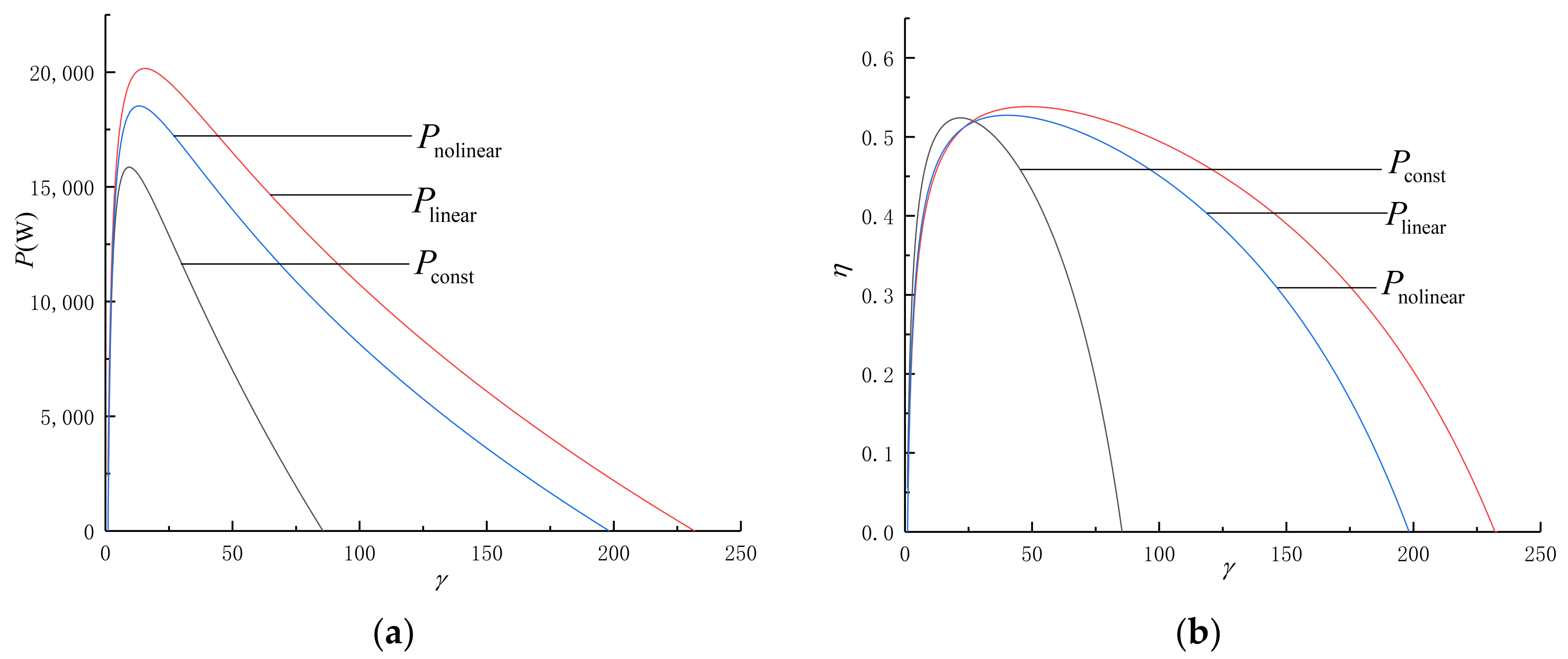
| Maximum Power Output | Maximum Value | Maximum Efficiency | Maximum Value |
|---|---|---|---|
| 15,858 | 0.5240 | ||
| 20,162 | 0.5383 | ||
| 18,527 | 0.5273 |
Publisher’s Note: MDPI stays neutral with regard to jurisdictional claims in published maps and institutional affiliations. |
© 2022 by the authors. Licensee MDPI, Basel, Switzerland. This article is an open access article distributed under the terms and conditions of the Creative Commons Attribution (CC BY) license (https://creativecommons.org/licenses/by/4.0/).
Share and Cite
Zang, P.; Chen, L.; Ge, Y. Maximizing Efficient Power for an Irreversible Porous Medium Cycle with Nonlinear Variation of Working Fluid’s Specific Heat. Energies 2022, 15, 6946. https://doi.org/10.3390/en15196946
Zang P, Chen L, Ge Y. Maximizing Efficient Power for an Irreversible Porous Medium Cycle with Nonlinear Variation of Working Fluid’s Specific Heat. Energies. 2022; 15(19):6946. https://doi.org/10.3390/en15196946
Chicago/Turabian StyleZang, Pengchao, Lingen Chen, and Yanlin Ge. 2022. "Maximizing Efficient Power for an Irreversible Porous Medium Cycle with Nonlinear Variation of Working Fluid’s Specific Heat" Energies 15, no. 19: 6946. https://doi.org/10.3390/en15196946
APA StyleZang, P., Chen, L., & Ge, Y. (2022). Maximizing Efficient Power for an Irreversible Porous Medium Cycle with Nonlinear Variation of Working Fluid’s Specific Heat. Energies, 15(19), 6946. https://doi.org/10.3390/en15196946