Water Level Control in the Thermal Power Plant Steam Separator Based on New PID Tuning Method for Integrating Processes

Abstract

The paper presents an analysis of water-level control in a thermal power plant (TPP) steam separator. This control structure is vital for the entire plant’s stable, reliable, and efficient operation. This process belongs to processes with an integrator because it concerns a level-control issue, and the control variable is the feedwater flow. Said industrial processes are challenging to control and apply standard methods for tuning the PID controller, so a new procedure has been proposed. A procedure for tuning a PID controller for integrating processes is proposed based on the IFOPDT model, obtained from the wide step response of the process. Based on the process parameters estimated, the tuning of the controller is proposed. Results from the TPP TEKO-B2 (350 MW) are presented as an experimental verification. Compared with standard tuning methods, better results are achieved in the form of rise time and disturbance elimination rate. A significantly less risky and faster experiment for parameter estimation and controller tuning is also obtained. In addition, one adjustable parameter is provided to select the relation between performance and robustness. This method can be applied to various industrial processes with an integrator.

1. Introduction

Thermal power plants are one of the most complex technological processes in terms of the production process complexity and the number of system components, including different technological processes, sensors, and actuators. Thermal power plants represent a significant source of electrical energy, and the reliability and efficiency of the entire system are essential for maintaining a stable supply chain to end consumers. This paper shall include the analysis of one of the critical thermal power plant subsystems, i.e., the water-level control subsystem in the steam separator of the Serbian TEKO B2 Drmno thermal power plant, with a nominal power of 350 MW. The implemented cascade control structure will be presented, and the process analysis will demonstrate that it is a process with an integrator. Control of such processes is significantly more difficult than processes without an integrator, so a novel method for tuning the PID controller parameters is proposed for efficient high-performance control. This paper is the result of many years of research in the theoretical domain but also is based on the practical implementation of control structures in more than 10 thermal power plants in Serbia with a power range from 100 MW to 650 MW.

During the design of the control, when the block reconstruction was carried out, the application of different control structures was considered. By analyzing the existing solutions, the present state of the industry [1], and the future system tuning and maintenance, a decision was made to use only PID controller-based structures. Considering recent analyses and comparisons of different types of controllers, taking into account the implementation options [2,3,4], we concluded that the right decision was made. Application of $H_{\infty }$ and a model-based predictive controller (MPC) requires an excellent knowledge of the process model, which is quite challenging to provide in this branch of industry. On the other hand, in case there is some change or disturbance in the system that can cause instability in the controller operation, the PID controller is easy to stabilize by changing the proportional gain. In contrast, for modern controller types, it is not so simple—the controller must be redesigned, which requires significant time and the presence of control engineers to redesign the controller.

With the conclusion that PID structures shall be used for control, a decision was made that it was necessary to perform a good tuning of the PID parameters to achieve good performance of the closed-loop system. Certain classical controller-tuning methods could not be implemented due to the inadequate experiments they required since it was a process with an integrator. Thus, the use of the relay-feedback method for determining the controller parameters was proposed, which was a good proposal, considering the available research [5]. The application of said method was proposed by Rotac [6] back in 1961, and since then, many different modifications and improvements have also been proposed [7,8,9,10,11]. However, based on the pulse response-based method [12], it was suggested to carry out further research and application options for a simpler and shorter experiment at a high-risk plant.

At the beginning of the 20th century, the first PID controller forms appeared, initiated by the practical need for precise navigation of large ships. Ever since, one has been able to find dozens of different schemes in the literature for both tuning the parameters of said controllers and characterizing the controlled process. The book by [13] discloses over 400 rules for controller tuning for different process types, including the step response-based procedure [14], but for processes without integrators. All of this indicates that none of the said structures is universal and that each process class requires special treatment. This paper describes a procedure that is demanding from two points of view. First, processes with an integrator are discussed, implying that the critical experiment from which the process parameters are read cannot last too long. Simultaneously, there are significant limitations on the control signal. In addition, the procedure is suitable for industrial processes, representing a different problem from the constant presence of various types of disturbances and non-negligible measurement noise. The authors believe that our experience, which becomes available to a wider community of electrical and mechanical engineers through this work, represents the missing segment in the range of various techniques for PID controller tuning. At the same time, we are sure that the presented results will arouse great interest among engineers who are in charge of designing and controlling industrial facilities, such as the water supply system in thermal energy blocks.

The water-level controlling process in steam separators is an extremely demanding design task for the following reasons. It is an integrator process translating the level from the minimum to the maximum in a very short amount of time. Therefore, the duration of every critical experiment from which the descriptive parameters of the process should be derived must be concise. On the other hand, the increment of the nominal control participating in the critical experiment must be minimal and carefully calculated. Then the measurement noise can be comparable to the useful signal. Considering the high pressure prevailing in the steam separator, one that is over 200 bar; the highly fluctuating boundary between steam and water; and the indirect level measurement by the pressure at the bottom of the separator, the measurement signal is very dynamic with a significant presence of measurement noise and measurement uncertainty. Finally, the water level in the steam separator is one of the safety protection signals at the thermal power plant, due to which the superior protection system, in a very short time interval measured in seconds, switches off the thermo-energy block according to the emergency procedure. In other words, the design requirements are rigorous, do not allow significant overshoot or undershoot, and require a fast response and elimination of disturbances. Therefore, this process was an inspiring motive for designing a new procedure for setting the PID controller parameters for processes with integral action.

The paper will demonstrate that the authors have been successful and have proven the initial hypotheses, namely, that it is possible to perform a suitable identification of the process parameters and, based on them, set the PID controller for the water-level control in the separator.

The paper has two significant contributions: (1) a novel method for tuning the process with an integrator, wide pulse-response tuning, is presented, and (2) the application of the water-level control procedure in the steam separator of the thermal power plant has been demonstrated. The efficiency of this new method, the simplicity of tuning, and the improvement of the performance over classic methods, is proven. Section 2 describes the steam separator-level control process at the TEKO B2 thermal power plant in Serbia, and the proposed and implemented control structure. Section 3 illustrates the new procedure for the PID controller tuning and theoretical analysis, and Section 4 presents experimental results and the process verification described in Section 2. Section 5 includes a discussion of experimental results and guidelines for further development, and Section 6 is the conclusion.

2. Process Description

Thermal power plants are the largest generators of electricity in Serbia, contributing to more than 65% of the overall power supply. As such, their operational efficiency and stability need to be maximized. Particular emphasis is placed on reliable long-term operation in terms of negotiated delivery commitments, operation per design criteria for energy efficiency, and longevity of the facility.

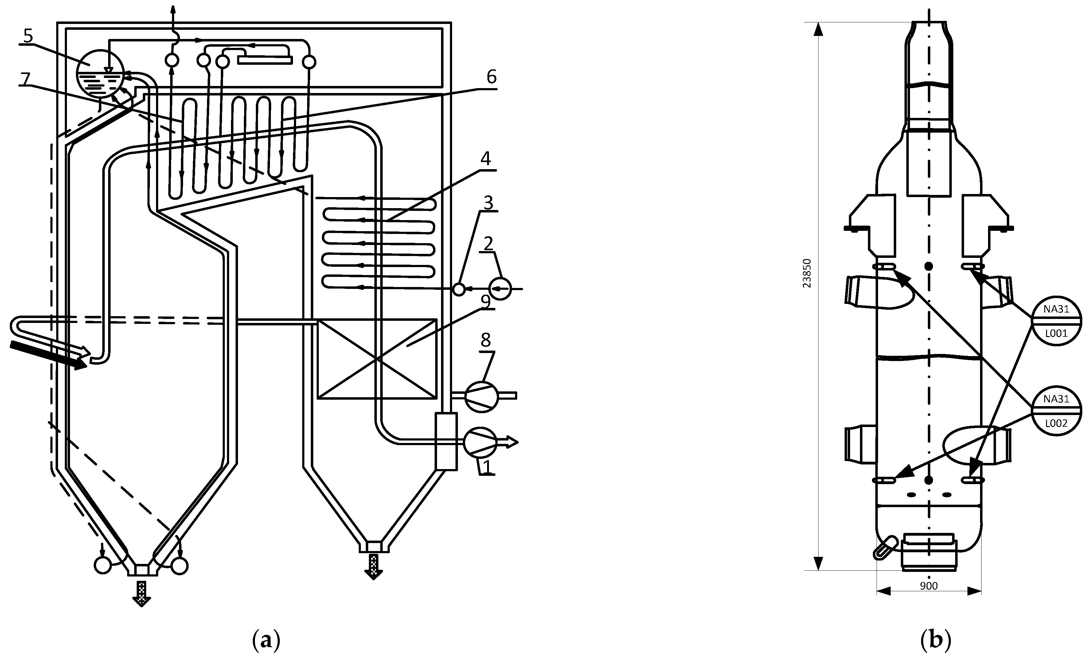
The paper addresses the control of the water-level steam separator (drum) in thermal power plant boilers [15,16,17]. A boiler is a unit in which the chemical energy of fossil fuel is converted into heat energy as steam. Figure 1a shows the basic structure of a steam boiler. Mills, usually six or seven, crush and grind coal, and then the controlled mixture of coal and preheated air is fed to a furnace via a system of ducts. In parallel, the oxygen needed for combustion is provided by an air-supply fan. The air is preheated to enforce combustion on the way to the boiler. Temperatures inside the boiler are as high as 1400 °C.

Feedwater pumps deliver preheated water to the steam drum via an economizer. Then additional pumps discharge the water into the system of pipes, where multi-stage heating takes place inside the boiler and the water is converted into steam. The steam separator also removes residual drops of water from the steam. The steam is then delivered to a multi-stage superheater, where it is heated to about 540 °C at a nominal pressure (usually 165–175 bars) before it leaves the boiler. The superheated steam flows to the turbine.

Specifically, at the TEKO B2 Unit of the Kostolac thermal power plant, nominal installed power is 350 MW, the diameter of the steam separator is 0.9 m, its height is about 24 m (Figure 1b), and it has a vertical orientation. Even a slight water-level variation inside the steam drum results in noticeable steam pressure fluctuations and affects the technical conditions of the process. If the water level is too high, emergency relief valves open to remove excess, but this measure reduces the unit’s operational efficiency. However, if the water level is too low, after a short time, the boiler shutdown procedure is initiated automatically to protect the piping and installation from overheating. As a result, precise control of the water level is very important for stable and efficient work of the entire powerplant.

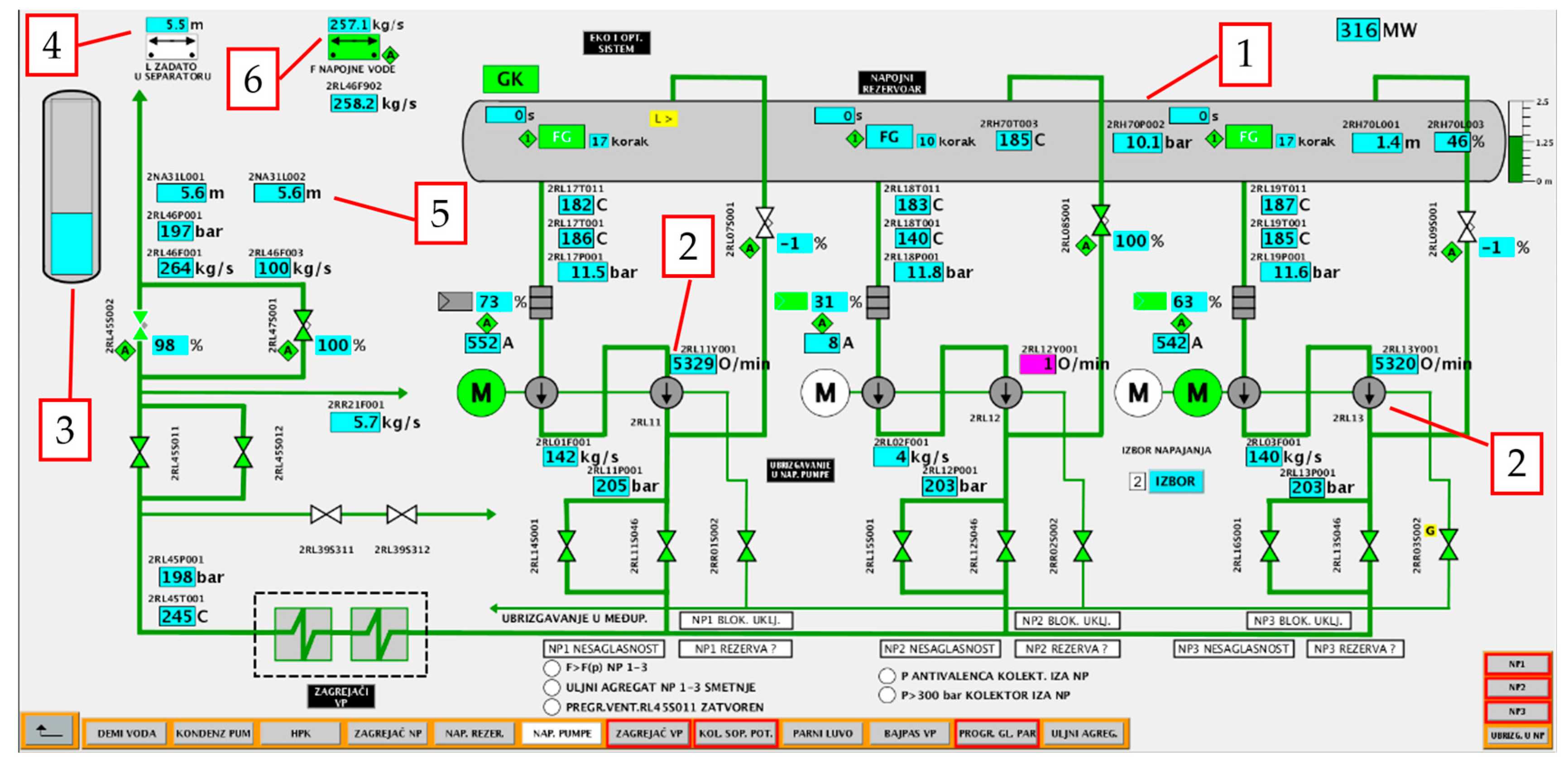
The feedwater subsystem is shown in Figure 2, which represents a realistic illustration of the SCADA system of the TEKO B2 Unit of the thermal power plant. Figure 2 shows the feedwater tank, three feedwater pumps (two of which are in operation, and one is spare), the main feedwater valve, and the steam drum (separator). Figure 2 shows all measured quantities in this subsystem: temperatures, levels, pressures, speed of pumps, actuator positions, and flows. Water from the feedwater tank is pumped via two pumps under high pressure (approx. 200 bar) into the steam separator (drum). Flow regulation is achieved through hydraulic couplings (manufactured by Voith) that receive the signal from the corresponding flow controllers, depending on the level in the separator. Then the feed water passes through the main feedwater valve, which keeps the pumps within the authorized operating mode, based on the pump protection Q-H curve, and reaches the steam separator.

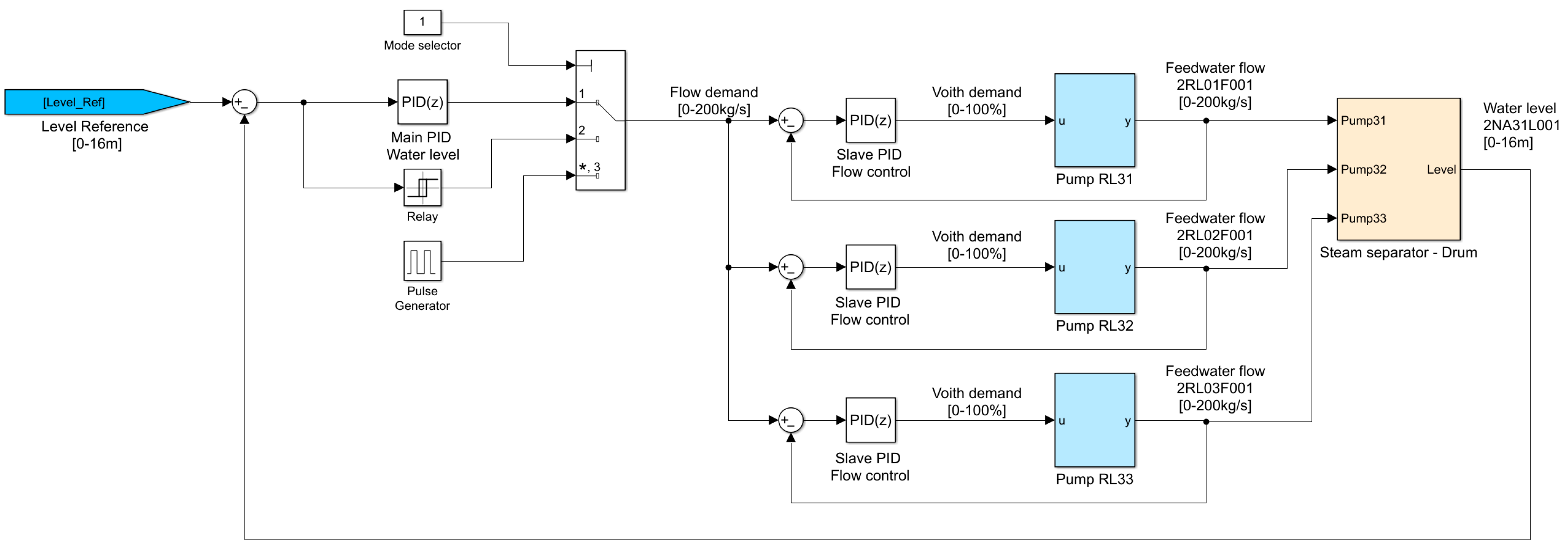
The control structure is shown in Figure 3, which is a cascade-level control. With the mode selector different modes can be chosen, as well as PID control and two modes for parameter estimation for controller tuning. This will be explained later in Section 4. The main level controller is a PID controller (value of mode selector set to 1) that regulates the water level in the steam drum (separator), and its control signal is the set feedwater flow rate for each pump. This regulator is basically the PD controller, and the integral action has been added to eliminate disturbances and maintain feedwater flow control—nominal operating mode. The set flow rate is passed to the subordinate (slave) PID controllers for each pump. Said controllers have the task of regulating the set flow for each pump (RL31, RL32, RL33) in operation via adequate hydraulic couplings (Voith’s). Their output signal is the Voith’s set load percentage, in the range of 0–100%. This control structure is chosen to manage multiple actuators (pumps) and distribute the controller’s functions into a level and flow control. The maximum performance of the control system is achieved as well as a high speed when changing the operating and spare pumps.

The water level in the steam separator (drum) depends on the water flow to the drum and the steam flow from the drum. Since an integrating effect is inherent in the process, the main controller must be adapted for process control with an integrator. The application of classic methods for the PID controller tuning is either not feasible due to the impossibility of conducting appropriate experiments or inferior performance. The settings obtained in this way lead to control systems that do not meet the efficient operation criteria for said subsystem. Therefore, it is necessary to resort to tuning the PID controller for controlling processes with an integral effect. To achieve maximum performance, ease of tuning, and the length of the experiment for obtaining the control parameters, a new method based on wide pulse response tuning (WPRT) is proposed, as presented in the following section.

3. New PID Controller Tuning Procedure for Integrating Processes—Wide Pulse Response Tuning (WPRT)

To identify parameters of the IFOPDT model (integrating first order plus dead time) represented by $G\left(s\right)=\frac{K}{s\left(Ts+1\right)}{e}^{-\tau s}$, it is necessary to determine the following parameters:

• $K$—gain;
• $T$—dominant time constant;
• $\tau$—transport delay.

For step excitation, the response of process with the integrator constantly increases or decreases depending on the sign of process gain, and theoretically is not bounded. In practical applications, the system’s output at some moment reaches a hardware limit due to plant constraints, limitations, or the protection system. Because of that, step response tuning does not apply to such plants and cannot be implemented in industrial practice.

If a process with only an integrator is observed, $G_1\left(s\right)=K/s$; as long as there is a constant input, the output of the process will rise. It will immediately stop rising at the end of step excitation, unlike the IFOPDT process output that does not stop increasing in the moment. This can be explained by the following: Steady-state time for the FOPDT processes is $\left(3÷5\right)T+\tau$ after every excitation change. Therefore, if the IFOPDT process $G\left(s\right)$ output is observed, part of it that represents FOPDT $\left(e^{-\tau s}/\left(Ts+1\right)\right)$ has an impact on the output $\left(3÷5\right)T+\tau$ after every step change of the input during a wide pulse experiment. This means that at the end of pulse excitation, $\frac{e^{-\tau s}}{Ts+1}$, which is part of $G\left(s\right)$, shall reach a new steady state after $\left(3÷5\right)T+\tau$, and that is one reason why the output will continue to rise after the end of wide pulse excitation.

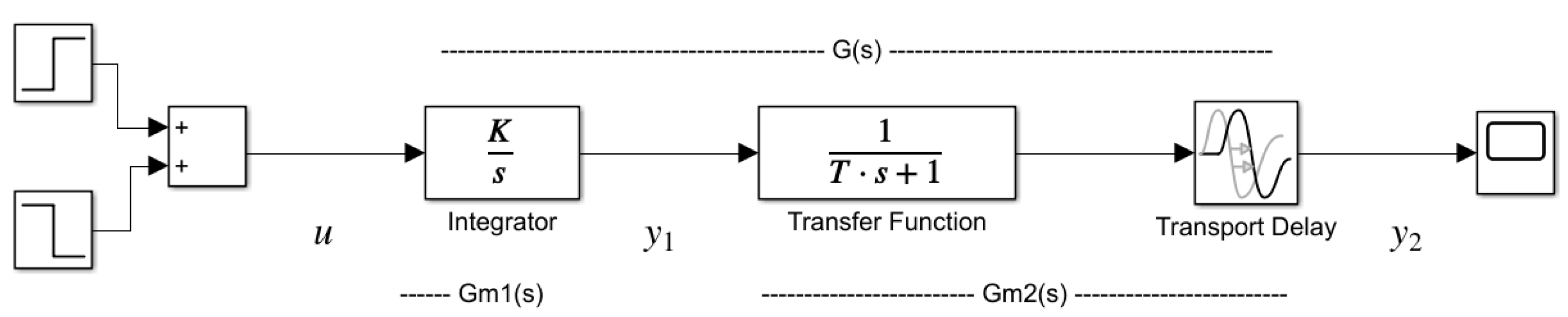
Transfer function $G\left(s\right)$, as shown in Figure 4, can be divided into two processes, connected in series $G_{m1}\left(s\right)=K/s$ and $G_{m2}\left(s\right)=e^{-\tau s}/\left(Ts+1\right)$.

If there is a constant step excitation $u$, $y_1$ (response of $G_{m1}\left(s\right))$ will be a function with a constant slope ($G_{m1}\left(s\right)$ is an integrator with gain). As for $G_{m2}\left(s\right)$, it will need $\left(3÷ 5\right)T+\tau$ to reach a new steady state, so ${\mathrm{y}}_2$, which is the output of $G_{m2}\left(s\right)$ and, at the same time, the output of the entire process $G\left(s\right)$, will be a pure ramp function after $\left(3÷ 5\right)T+\tau$ time.

Now the second part of the IFOPDT model can be observed. $y_1$ is a ramp excitation for the process $G_{m2}\left(s\right)$. After reaching the ramp signal on ${\mathrm{y}}_2$, which means that $G_{m2}\left(s\right)$ has reached steady state, pulse excitation is suspended, e.g., the process input has previous values before the experiment is started. Then, $y_1$ reaches the last value before excitation is stopped, and it maintains that value. As for $G_{m2}\left(s\right)$, whose input is $y_1$, the above mentioned process represents step excitation with a value of the difference of $y_1$ and $y_2$(further $\Delta y$) at the end of the pulse. The $y_2$ signal will increase its value until $G_{m2}\left(s\right)$ reaches a new steady state (which is the value of $y_1$ at the time of the change).

The main idea is to determine the dynamic parameters of the IFOPDT model, $\tau$ and $T$, by measuring the time required for the process to reach 10% and 63% of the response. Model gain $K$ can be obtained as the ratio of a total change of output $y$ and the area of wide pulse excitation $A$. This will be discussed in detail in the next two subsections.

In industrial practice, we often encounter two process types, those with no or with negligibly small transport delay or those that have a significant transport delay. Therefore, to determine the parameters of the IFOPDT model, two separate cases must be considered. After the conducted open-loop experiment with wide step excitation, the process’s output is observed. If there is a change in the output in a short time interval, we can talk about a process with no or negligibly small transport delay. If the output change does not occur during a short amount of time, then the case of a process with a significant transport delay must be considered.

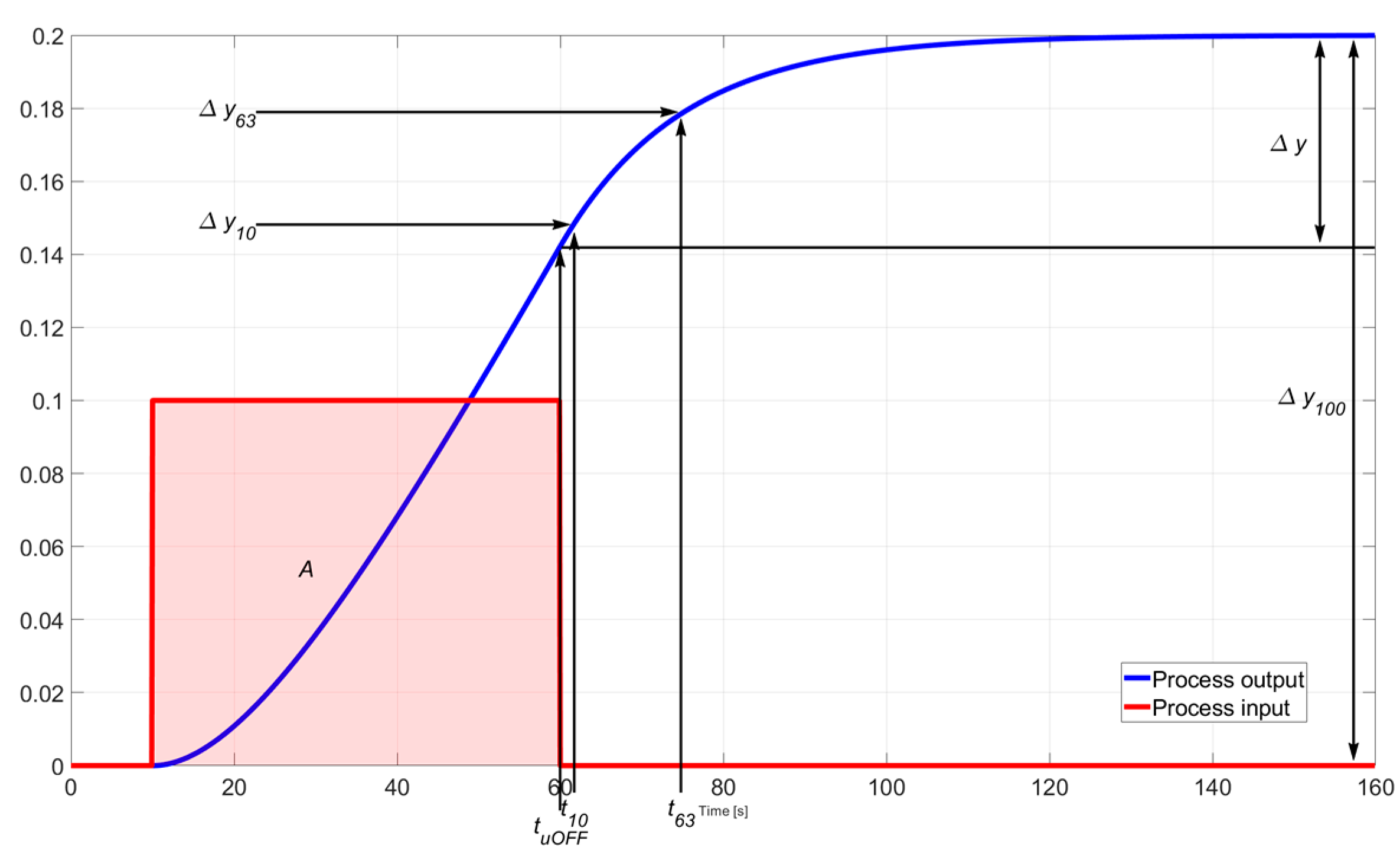
3.1. Process with Small or No Transport Delay

If a process with small or no transport delay is considered (as shown in Figure 5), the parameters of the IFOPDT model can be obtained by the following procedure:

• The time delay of the IFOPDT model $\tau$ can be obtained by measuring the time required for the process response to reach 10% of $\Delta y$, marked as $t_{10}.$ Therefore, the delay is calculated as $\tau =t_{10}-t_{u\mathrm{OFF}}$, wherein $t_{u\mathrm{OFF}}$ is the moment when the excitation ends;
• The equivalent time constant $T$ is the time for the response to change from 10% to 63% of $\Delta y$, $T=t_{63}-t_{10}$;
• Process gain $K$ can be determined as mentioned as the slope of the reaction curve (system output), or more robustly as the ratio of a total change of output and area of wide pulse excitation $A$,$K=\mathsf{\Delta }{y}_{100}/A$.

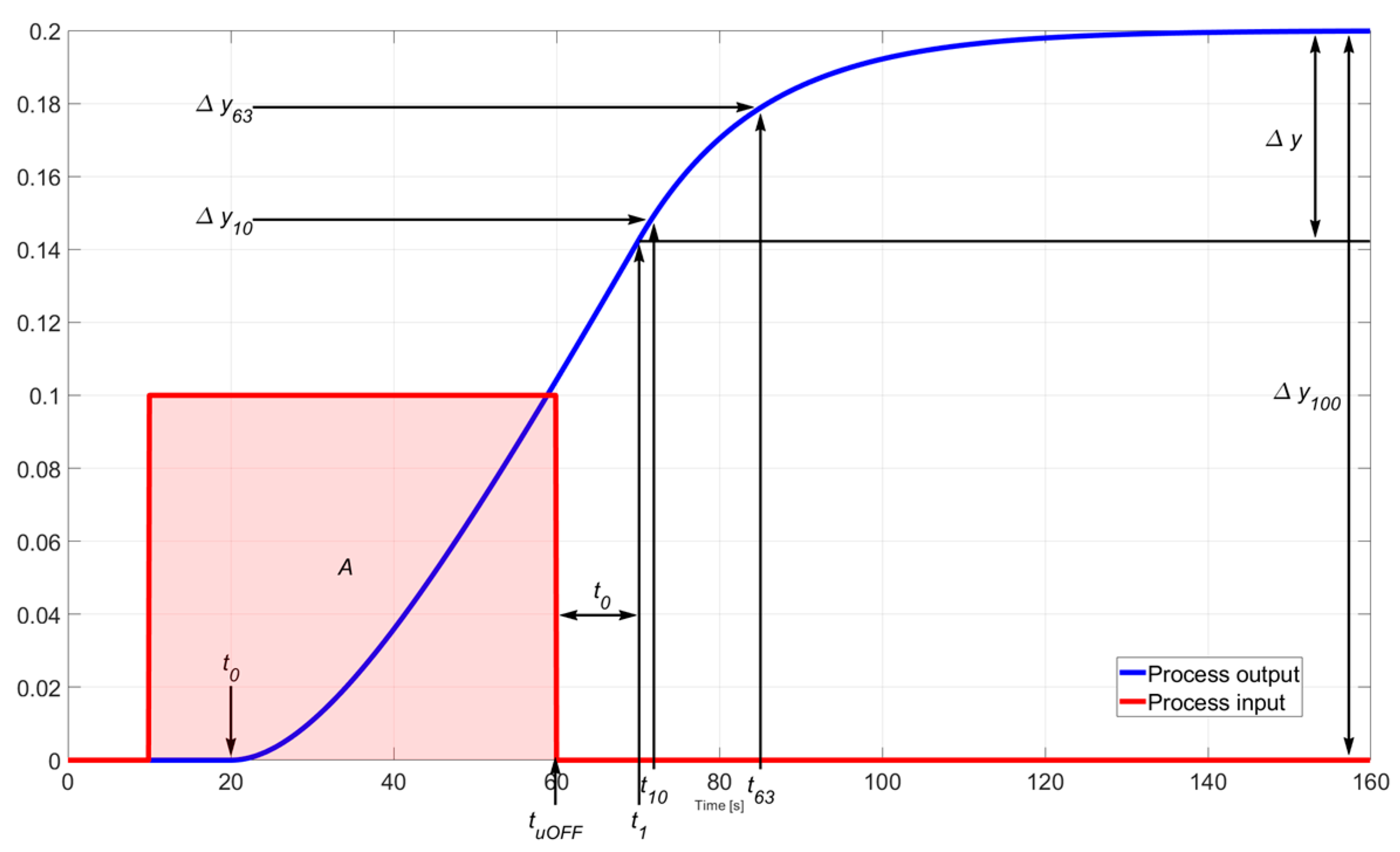
3.2. Process with Moderate or Significant Transport Delay

If the process has a transport delay that cannot be neglected (as shown in Figure 6), the IFOPDT model parameters can be obtained by the following procedure:

• The time delay of the IFOPDT model $\tau$ can be obtained as a sum of the delay $t_0$ and time $t_{10}-t_1$. Time $t_1$ is defined as the sum of wide pulse end time $t_{uOFF}$ and $t_0$, $t_1=t_{uOFF}+t_0$. Time $t_{10}$ is calculated by measuring the time required for the process response to reach 10% of $\Delta y$;
• The equivalent time constant $T$ is the time for the response to change from 10% to 63% of $\Delta y$, $T=t_{63}-t_{10}$;
• Process gain $K$ can be determined as mentioned as the slope of the reaction curve (system output), or more robustly as the ratio of a total change of output and area of wide pulse excitation $A$,$K=\mathsf{\Delta }{y}_{100}/A$.

3.3. PID Tuning Rules

For processes with the integrator, a PD controller should be used. Due to load rejection and setting nominal regime, the integral part will also be included, but integral time should have a high value according to process time constant $T$.

The structure of the PID controller is defined as:

$$G_{PID}=K_p\left(1+\frac{1}{T_{i}s}+\frac{T_{d}s}{T_{f}s+1}\right).$$

(1)

First, the controller will be observed as simple PD, ${\mathrm{G}}_{\mathrm{PD}}\left(\mathrm{s}\right)=K_p\left(1+T_{d}s\right)$. After determining $K_p$ and $T_d$, filtering of differential action $T_f$, the integral term of the PID controller $T_i$ will be introduced and it will be assumed that they do not have a lot of influence on stability and system performance. By introducing the integral action, the order of astatism of the system increases, and the stability of the closed-loop system, generally speaking, may be impaired. With certain approximations, it can be shown that by introducing the integral effect, the transfer function in the open-loop discrete system gets a pole at the point $p=0$ and zero at the point $z=-1/T_i$. By choosing a sufficiently large $T_i$ parameter e.q. $T_i\ge 10T$, it is possible for this pole and zero to be close enough to each other, but also far enough from the point ${\omega }_1$ (frequency of phase margin) so that their influence on the phase margin, and consequently the stability, becomes almost negligible.

The steps for determining the PD parameters are based on [12,14]. The differential time constant $T_d$ is taken to be

$$T_d=T,$$

(2)

where $T$ is the equivalent time constant of the process, evaluated as shown in Section 3.1 and Section 3.2. Then open-loop transfer function is:

$$W\left(s\right)=G\left(s\right)G_{PD}\left(s\right)=\frac{K}{s\left(Ts+1\right)}{e}^{-\tau s}{K}_p\left(1+T_{d}s\right),$$

(3)

$$W\left(s\right)=\frac{K{K}_p}{s}{e}^{-\tau s}.$$

(4)

The pole of the process $\mathrm{G}\left(\mathrm{s}\right)$ is canceled by proportional and differential action of the PD controller $\left(1+T_{d}s\right)$. The proportional gain of the PD controller $K_p$ remains to be determined, which can be determined by applying the Nyquist stability criterion to the characteristic equation

$$1+W\left(s\right)=1+G\left(s\right)G_{PD}\left(s\right)=1+\frac{K{K}_p}{s}{e}^{-\tau s}=0.$$

(5)

Choosing $K{K}_p$ to obtain the desired phase margin ${\varphi }_{pm}$ [14,18,19] gives

$$K_p=\frac{\mu }{K\tau }$$

(6)

$$\mu =\frac{\pi }{2}-{\varphi }_{pm}$$

(7)

where ${\varphi }_{pm}$ is the desired phase margin [16,17].

Parameter $\mu$ is chosen to be in the range $\mu \in \left(0.32,0.54\right)$. A higher value of $\mu$ results in better performance, more aggressive control, and less robustness.

The integral term of the PID controller $T_i$ is introduced in the controller for good load rejection and regime changing. It should have a significantly higher value than the process dynamic but small enough to preserve good disturbance rejection [19], and the adoption of the value $T_i=10T$ is suggested.

To avoid aggressive control caused by a high gain of differential action $T_d$, a filter for a differential part is used, with the time constant $T_{fd}=T/n_d$. Parameter $n_d$ is chosen from the range $n_d\in \left(5,10\right)$. Lower $n_d$ values are better for good filtration of measurement noise and higher values for stability because the filter has less influence on the closed-loop process. It is a heuristic recommendation, and it is formed in such a way as to make a compromise between noise-measurement filtering that can cause significant damage when realizing the differential effect of the PID controller and preserving the system’s dynamics. Paper [20] analyzed various filters and parameters, and the authors of this paper chose the proposed one due to the implementation simplicity and the intuitiveness of the setting parameter. It is up to the system designer to find a compromise between these two conflicting requirements. The recommendation is that $n_d$ be between 5 (when it is up to the dynamics of the system) and 10 (when the measurement signal filtration is more important) as the range that the authors consider satisfactory, after many experiments with different systems. The recommended value of $n_d=10$ can be adopted during implementation, and if the control is too aggressive, the value of $n_d$ can be reduced to 5.

3.4. Simulation Results of the Proposed Tuning Procedure

As an example, for comparison with IMC-PID [21], $G_p=\frac{0.004}{s\left(15s+1\right)}{e}^{-\tau s}$ will be used. IMC-PID (internal model control–PID) is the controller-tuning procedure known in the literature [22] and frequently used in industrial practice. The author’s idea was to compare the result of the proposed controller with the result of this well-known tuning procedure.

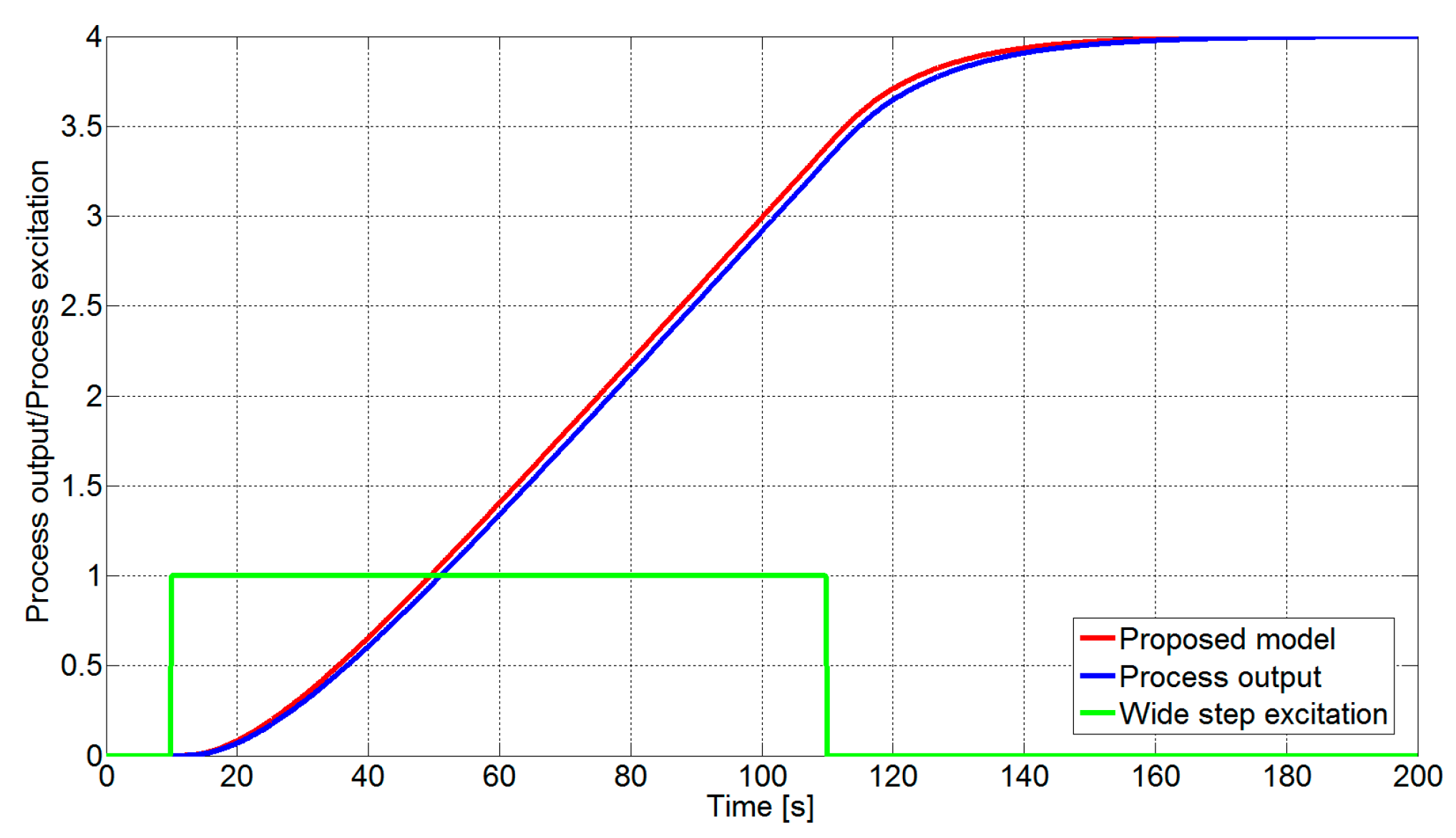
First, it is necessary to model the process and identify parameters of the proposed IFOPTD model. In $t=10 \mathrm{s}$ wide pulse excitation is started (Figure 7). From the process response, it can be seen that the process had no significant time delay. In this example, the duration of the wide pulse excitation was $\Delta t=100\mathrm{s}$. At $t_{uOFF}=110\mathrm{s}$, pulse excitation ended. Then, the time constant and the transport delay could be calculated as in the proposed procedure.

Process gain is estimated as the ratio of the process output change and the area of wide pulse excitation on the process input $K=\mathsf{\Delta }{y}_{100}/A$. Area $A$ is defined as a product of wide pulse excitation duration $\mathsf{\Delta }t=100s$ and excitation magnitude $u=10$, so $A=1000$. The final value of the process output is $\mathsf{\Delta }{y}_{100}=4$. The estimated parameters of $G_p$ are as follows:

$$K=0.004,T=13.5,\tau =1.8$$

(8)

Figure 7 shows promising results of the proposed IFOPDT modeling for a process chosen in [21]. The main goal for the controller is to satisfy two opposite demands: to have high robustness and good performance, so for analysis, parameter $\mu$ was chosen to be $\mu =0.32$ and $\mu =0.54$, for good robustness and good performance, respectively. Parameter $T_d$ was chosen to be identical to the estimated time constant, $T_d=T$. For filtering differential action, the time constant of the filter $T_{fd}=T_d/5$ was chosen. It was high enough to suppress the impact on the PD output but at the same time small enough not to affect the process’s dynamic. Reasons for introducing an integral part in the controller have been mentioned. The time constant of integral action $T_i$ was chosen to be much higher than the process dynamics, $T_i=10T$. Thus, the parameters of the PID controller were

$$K_p=44.4\left(\mathsf{\mu }=0.32\right),K_p=75.0\left(\mathsf{\mu }=0.54\right),T_d=13.5,T_i=135,T_{fd}=2.25.$$

(9)

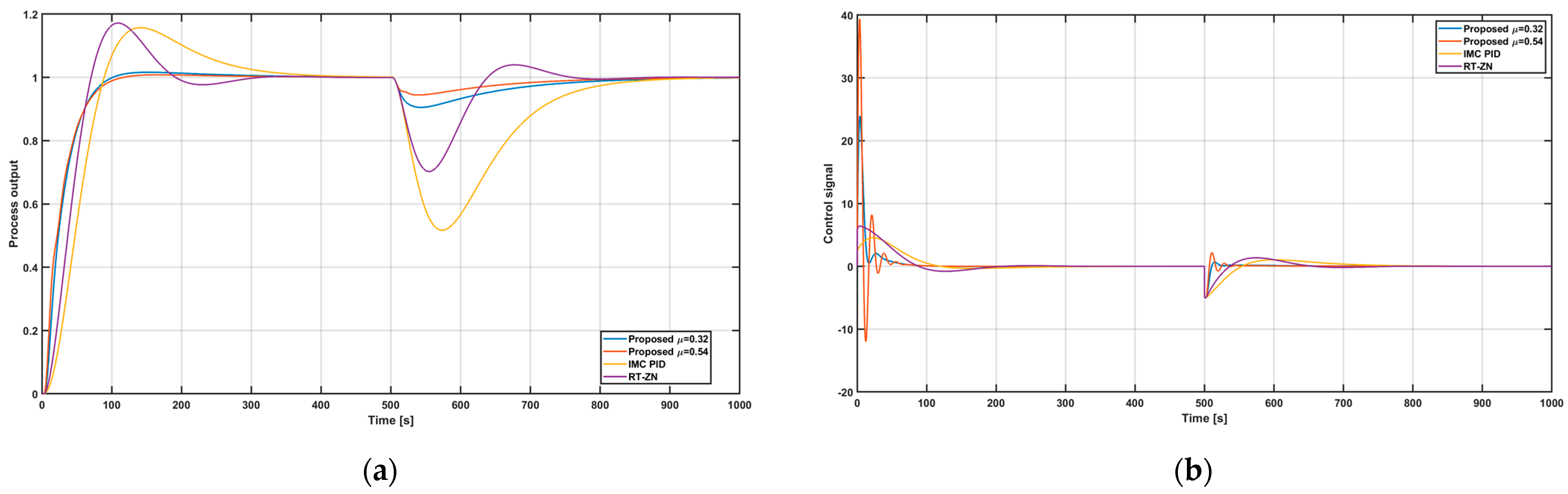
Figure 8 shows a comparison between the proposed procedure for two values of tuning parameter $\mu$ and the tuning presented in [21], also suggested for integrating processes and classical Ziegler Nichols tuning, based on a relay experiment [23].

A disturbance is introduced as a step signal on the process input in the middle of simulation, $t_{dist}=500\mathrm{s}$. Good disturbance rejection of the proposed tuning method can be seen in Figure 8, as a result of a good selection of the integral time, $T_i=10T$.

4. Experimental Results and Verification

To carry out the experimental verification of the proposed method based on wide pulse response, preparation for experimental tuning was carried out. Namely, two methods were selected for comparison, the proposed WPRT and the classic Ziegler Nichols method, with the identification of process parameters using the relay-tuning procedure. In the case of the water-level control in the steam drum (separator), the control structure for the two experiments is shown in Figure 3, in such a way that by selecting the operating mode, one chooses the control via the PID controller (mode 1), relay experiment (mode 2), and wide pulse (mode 3).

• Mode 1—PID operating mode.
• Mode 2—mode for obtaining the tuning parameters by the ZN method, so-called relay tuning (RT-ZN). In this mode, an error signal is fed to the input of the relay, which is formed as the difference between the setpoint level and the level measured in the separator, and the control signal is generated at the output of the relay, which is forwarded to the flow regulators of the pumps. In this way, controlled self-oscillations are obtained in the system, the basis for determining the parameters $K_u$ and $T_u$ for the PID controller tuned by the ZN method. To make the method reliable for identifying the amplitude and period of the oscillations, it is necessary to wait for the formation of self-oscillations and their duration of at least five periods. This requires a certain amount of time necessary for careful monitoring of the experiment. If the output value of the level exceeds some values set as dangerous for the process, it is required to take over manual control and bring the process into the safe operating zone.
• Mode 3—mode for applying the WPRT method implies breaking the feedback loop, using a constant control signal from the last period of automatic operation, setting a step excitation signal, and waiting for the appropriate time. Then the excitation returns to the previous level. After the end of the transition regime, as described in the previous section, the process returns to the automatic operation mode.

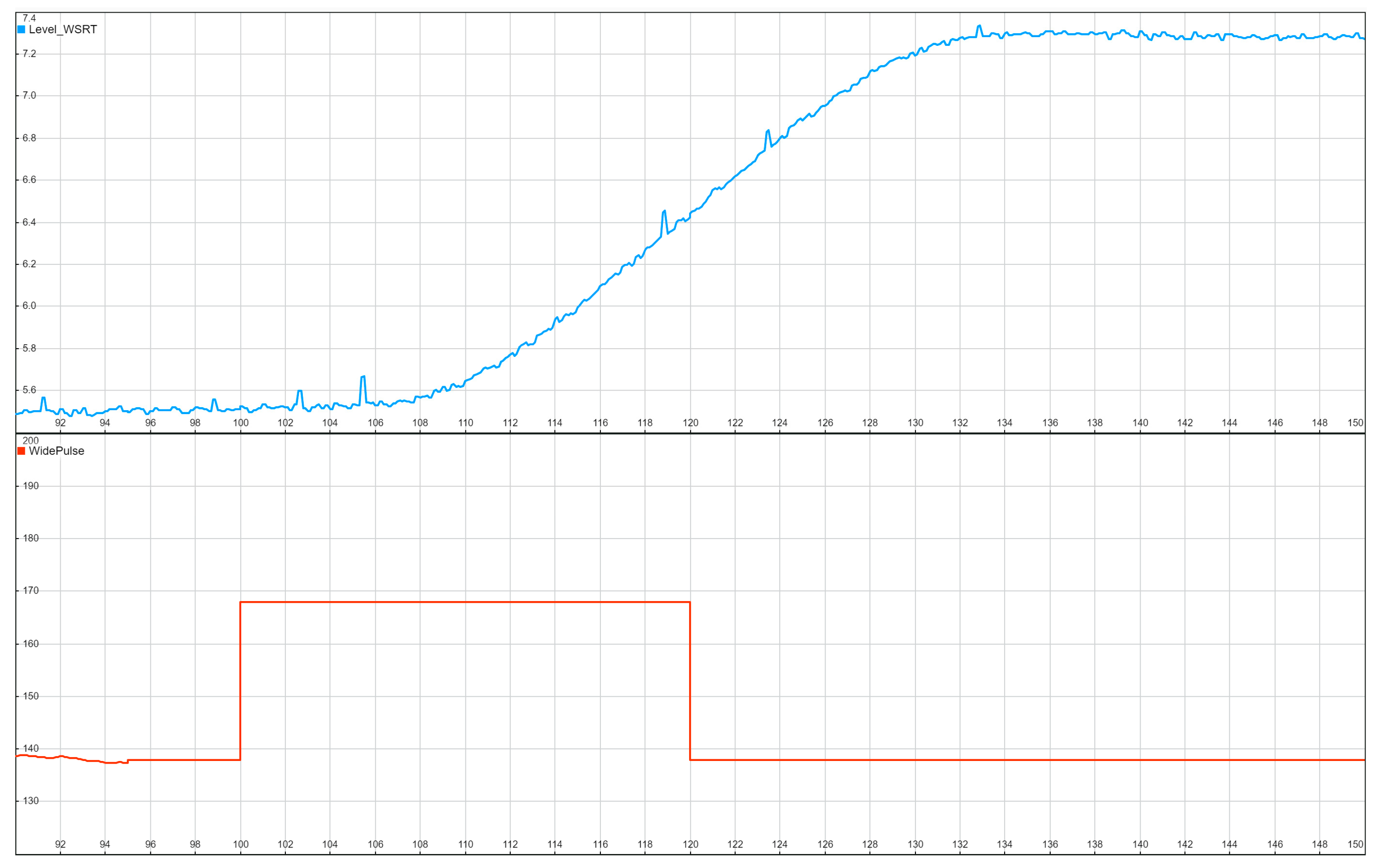
The obtained measurements and time response for the proposed WPRT method are shown in Figure 9. The system was switched to manual mode at t = 95 s, with the feedwater flow per pump set at u =138 kg/s. A pulse was set at $t_{uON}=100 \mathrm{s}$ with an amplitude $\mathsf{\Delta }u=30 \mathrm{kg}/\mathrm{s}$ and duration $t_{pulse}=20 \mathrm{s}$. The water level in the steam separator ranged from 5.5 m to 7.3 m, which was within acceptable limits for reliable operation. The automatic operation mode was set again at $t=150\mathrm{s}$. Based on this experiment, the IFOPDT model parameters were determined as suggested in the previous section, and then the PID controller parameters were determined. As it is necessary to achieve maximum performance in this subsystem, the parameter $\mu =0.54$ was selected, and the following PID controller parameters were obtained

$$K_p=36.7, T_i=35, T_d=3.5, T_{fd}=0.7$$

(10)

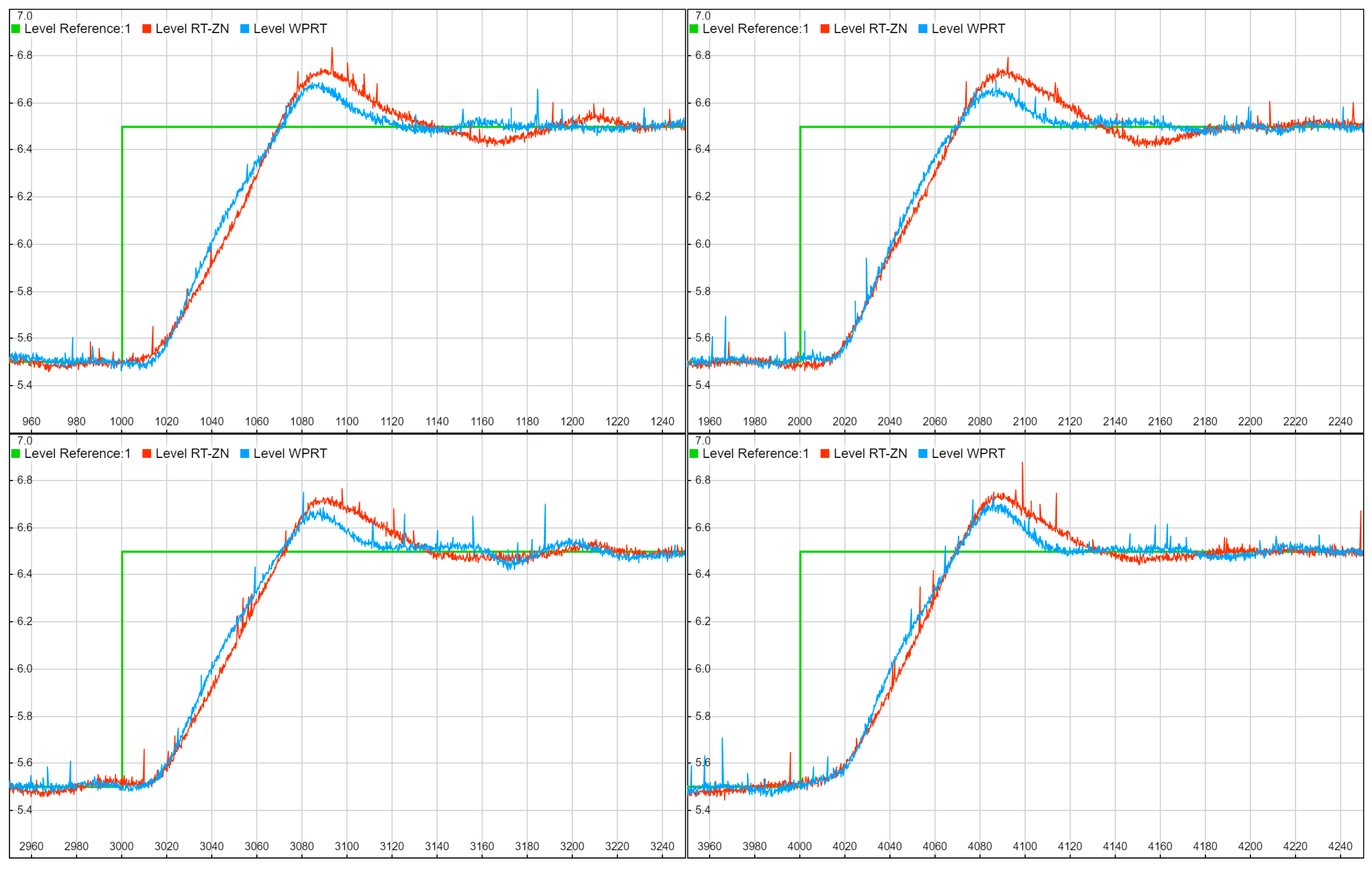
After PID controller tuning with two methods, RT-ZN and WPRT, the following comparative experiments were performed, at the same nominal power of the plant and in the quiet operation of the block, without major disturbances:

4

Reference change test: The water level setpoint in the separator was changed from 5.5 m to 6.5 m.

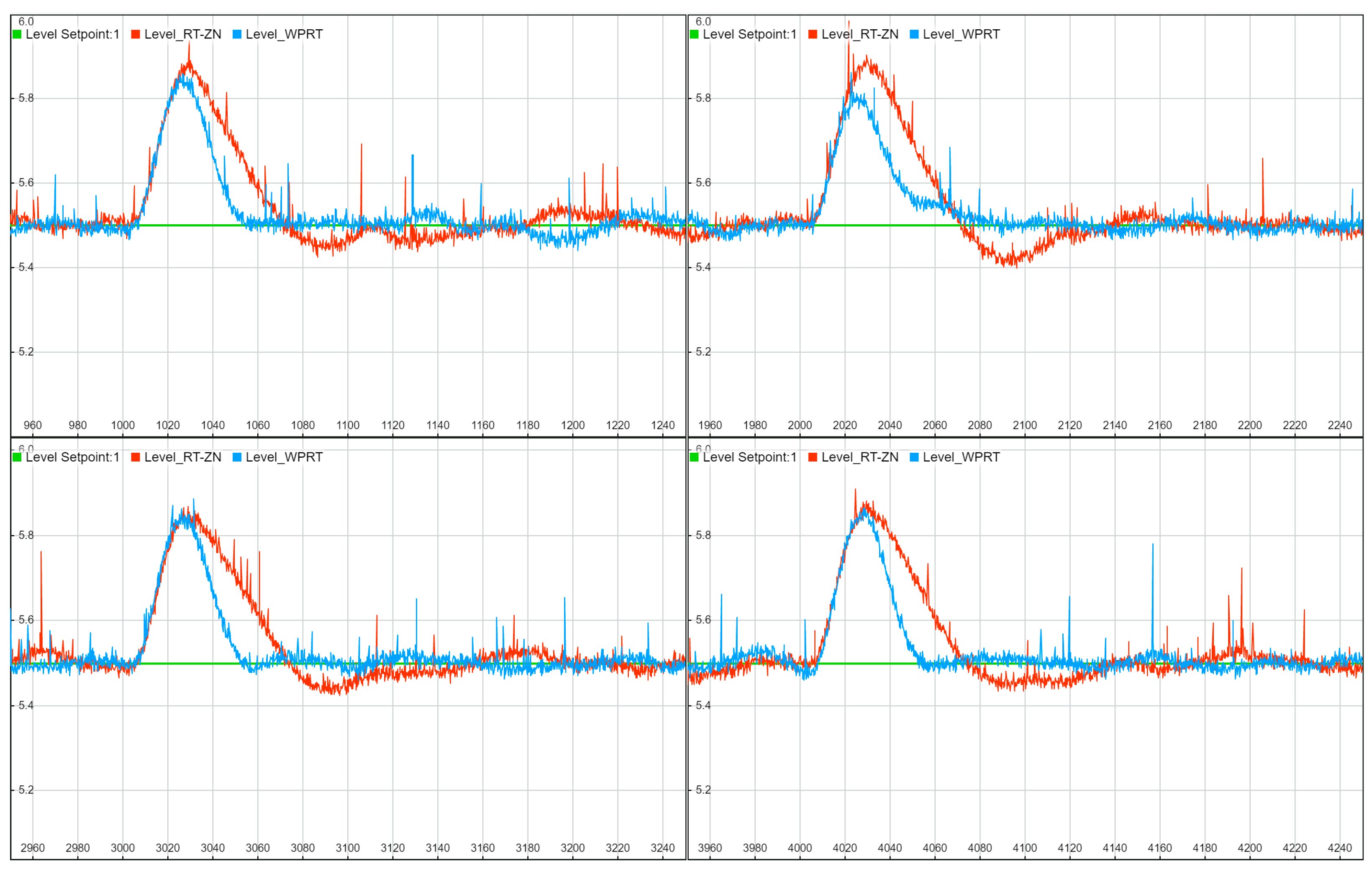
5

Process input disturbance test: The output of the controller, the flow rate of the feed water for the slave controller, was increased by 10 kg/s.

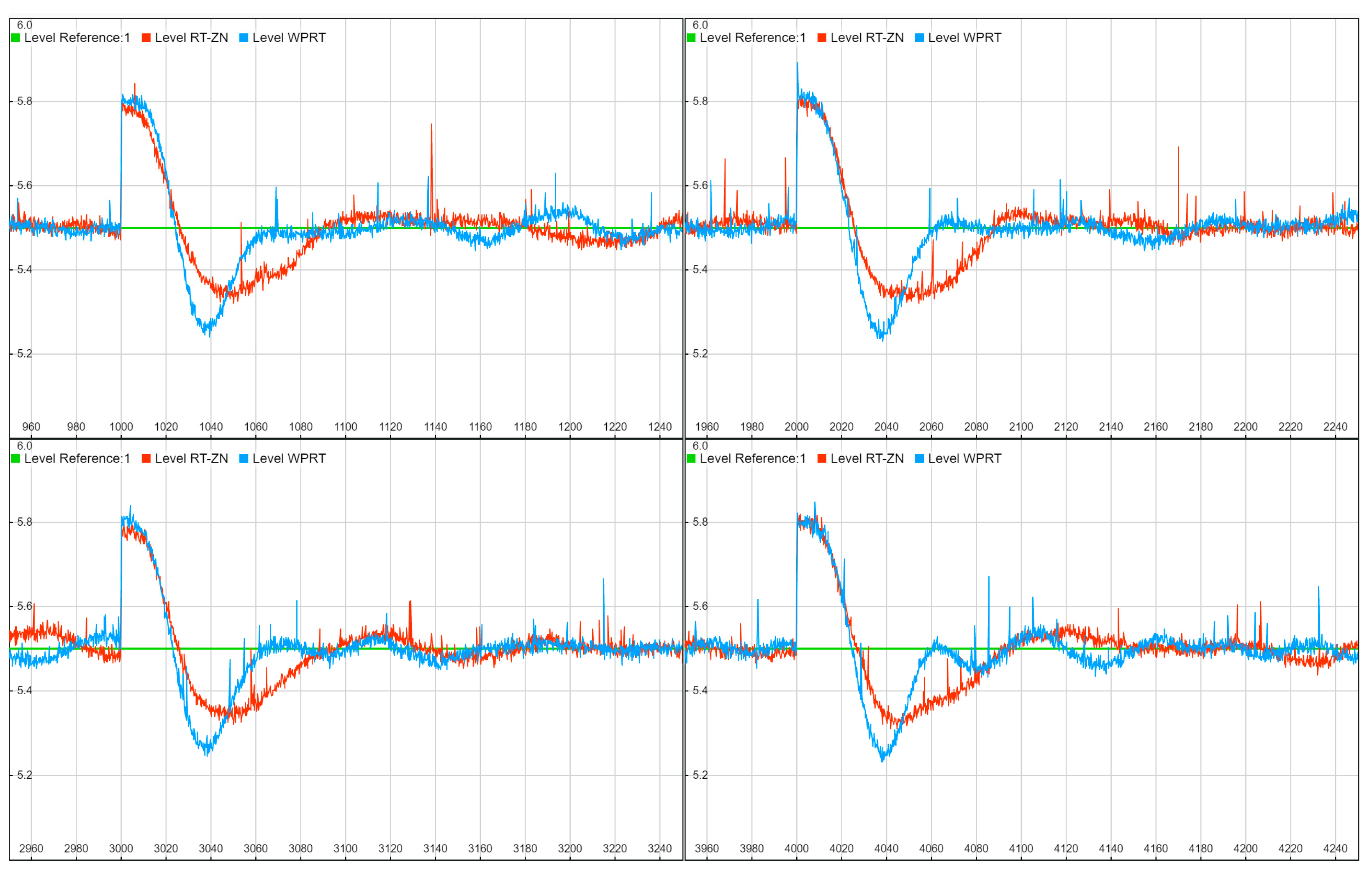
6

Process output disturbance test: At the output of the process, the level measurement itself was increased by 0.3 m.

7

Controller nominal operation test: In the nominal operation mode, the control deviation was recorded to compare the two settings of the controller.

All tests lasted 250 s and were repeated four times with both controller settings, with alternating repetitions, since there are always minor disturbances in the process caused by uneven coal quality, uneven combustion, and many other parameters. To assess the control quality, the integral absolute criterion was applied, $IAE=\int \left|e\left(t\right)\right|\mathrm{d}t$, which had the control deviation as an input $e\left(t\right)=r\left(t\right)-y\left(t\right)$. The control signals had to be realistic since there were slope limiters in the system that did not allow the control signal to rise or fall too much. It should be noted that all signals were recorded by the primary sampling time that the DCS system itself operates with, $T_s=0.2 \mathrm{s}$.

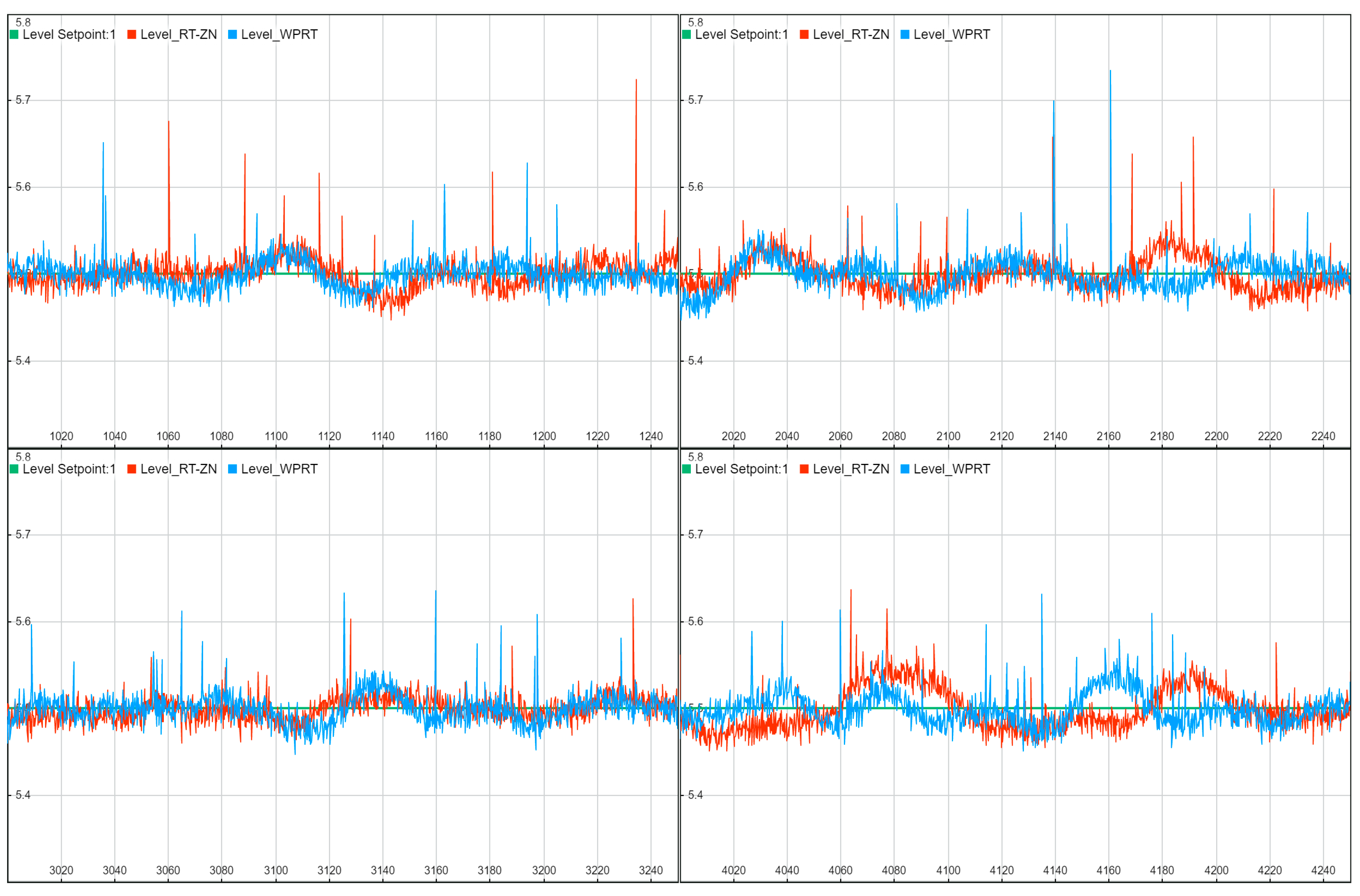
The following Figure 10, Figure 11, Figure 12 and Figure 13 illustrate time diagrams for four experiments for each controller. They can be used to compare the time responses and the control quality for the classic RT-ZN method, and the proposed WPRT method in actual application (real conditions) in an extremely complex process being controlled.

5. Discussion

After thoroughly conducting experiments in an existing plant facility, it is possible to perform a results-based analysis.

Table 1. Table of comparative results of integral absolute error (IAE) for four different experiments, each repeated four times.

Test Type	Setpoint Change IAE		Input Disturbance IAE		Output Disturbance IAE		Nominal Regime IAE
Test No	WPRT	RT-ZN	WPRT	RT-ZN	WPRT	RT-ZN	WPRT	RT-ZN
1	47.44	54.80	11.82	17.18	13.96	14.64	2.90	3.21
2	46.78	54.52	10.78	17.82	13.31	14.75	3.57	3.85
3	48.15	53.69	11.07	17.02	12.78	13.52	3.18	2.77
4	47.69	53.02	10.89	17.06	14.26	15.28	3.80	5.04
Average	47.52	54.01	11.14	17.27	13.58	14.55	3.36	3.72

shows in detail the values of the IAE criteria for each type and for each experiment repetition. The last row shows the mean values for each experiment for both methods.

The lower value of the IAE criteria for the proposed WPRT method is evident compared to the tuning based on the relay-tuning experiment (RT-ZN), which is common in practice.

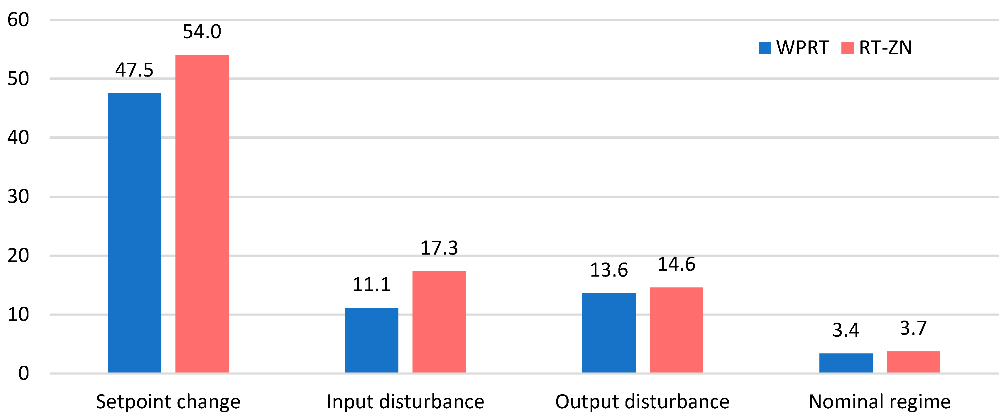
Figure 14 shows a comparative illustration of the IAE criteria mean values for individual experiments. Lower criteria values reflect a better behavior of the controller in operation, and the consistency of improvement for all proposed tests should be emphasized. Thus, the better performance of the proposed WPRT method is unequivocally demonstrated. This claim is supported by the results obtained during the theoretical analysis of the control quality of several controllers, as shown in Figure 8. Since there were no options for a large number of experiments to be conducted in practical conditions, the comparison was made only with the RT-ZN method, the method often used in practice, which showed promising results in the previous analysis. It should be noted that the control signals are not shown because they were limited by rate limiters located before the actuators (Voith’s hydraulic couplings). Therefore, they did not affect the analyzed results.

For future research, signal-processing methods and measurement filtering should be considered. As visible from the signals from the plant, there was an evident level of noise that affected the quality of parameter estimation (Figure 9), and the particularly problematic issue is that this noise did not have Gaussian distribution. Namely, bubbles often developed in the steam separator in water, traveling to the surface and being detected by the level sensor as peaks. It is necessary to carry out high-quality data pre-processing but in such a way as not to affect the dynamics of the signal, because it could affect the estimation of the IFOPDT model parameters. Recently, many deep learning-based methods [24,25,26,27] have been developed, so it is necessary to perform an analysis and try to apply them in industrial practice.

6. Conclusions

The paper presents a novel method for the PID controller parameter tuning for control processes with the integrator. This type of process is complicated and challenging to control because instability and poor performance are typical with controllers tuned using conventional tuning procedures. Within the proposed WPRT, clear instructions have been provided for conducting a quick, simple-to-understand, and easily controlled experiment to obtain the IFOPDT model parameters. After identifying the parameters of the model, tuning of the PID controller is performed, with one free tunable parameter available, which can be used to choose between better performance or robustness.

During the actual process of the water-level control in the steam separator at the thermal power plant, the controller tuning procedure is demonstrated. A comparative analysis with a classically tuned controller using a relay experiment is provided. The results of the plant operation show significantly better results than the method proposed herein.

The proposed WPRT method can be effectively applied to a wide range of industrial processes that include the integrator, usually level controllers, and positional servo systems. The proposed method proved to be better in all aspects of the application: from the simple experiment to the behavior of the controlled output value, but also due to the possibility of additional tuning by using a free parameter. The authors believe that this paper represents the missing segment in the range of various techniques for PID controller tuning, especially for designing and controlling industrial facilities, such as the water-supply system in thermal energy blocks.