
A Review of Reliability and Fault Analysis Methods for Heavy Equipment and Their Components Used in Mining


Abstract
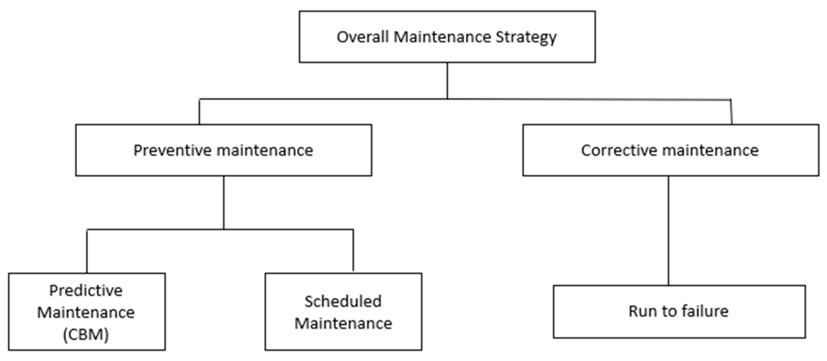
:1. Introduction
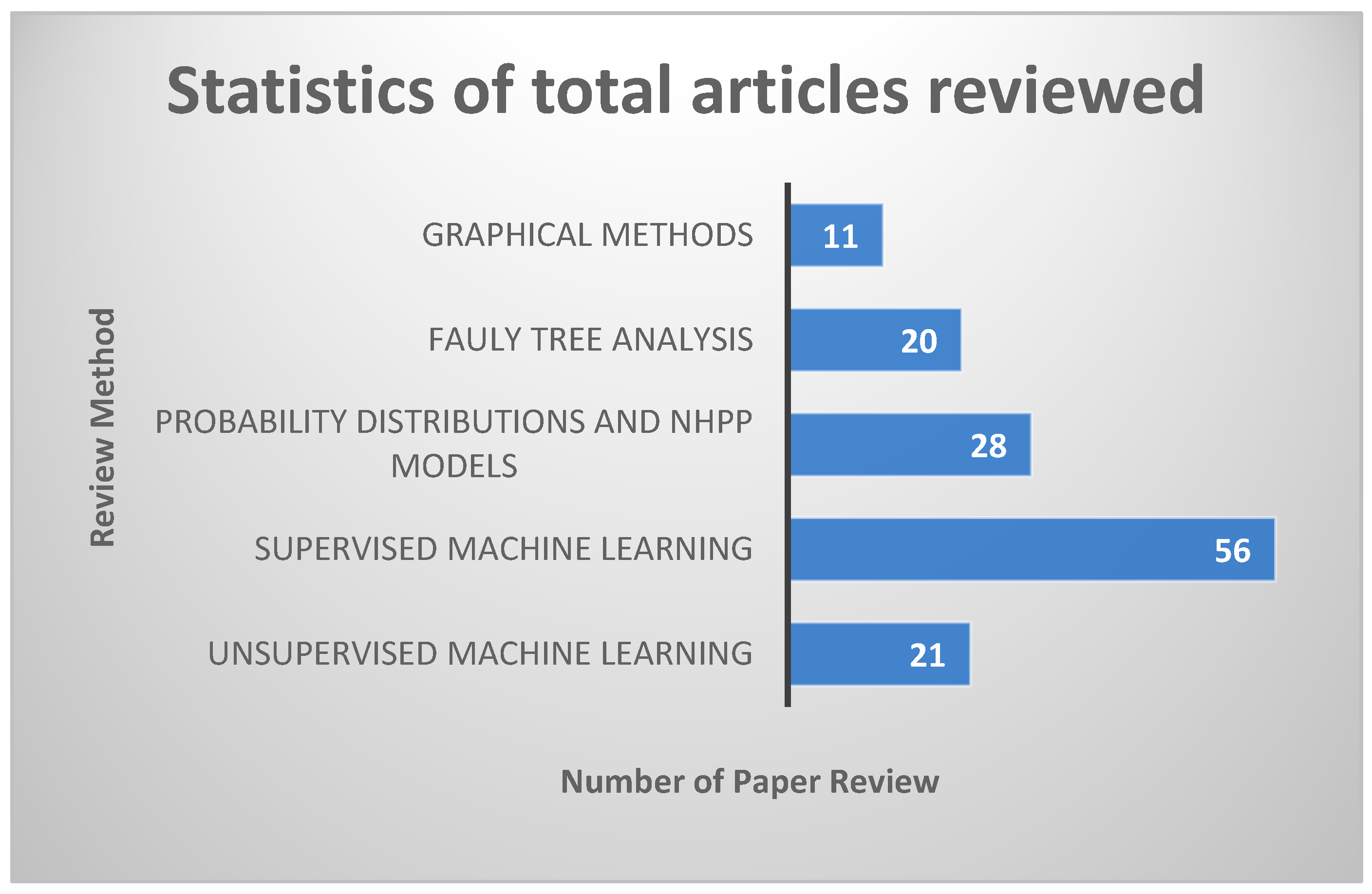
2. Methodology
3. Review on Application of Different Traditional Methods Used in Reliability and Fault Analysis
3.1. Graphical Methods
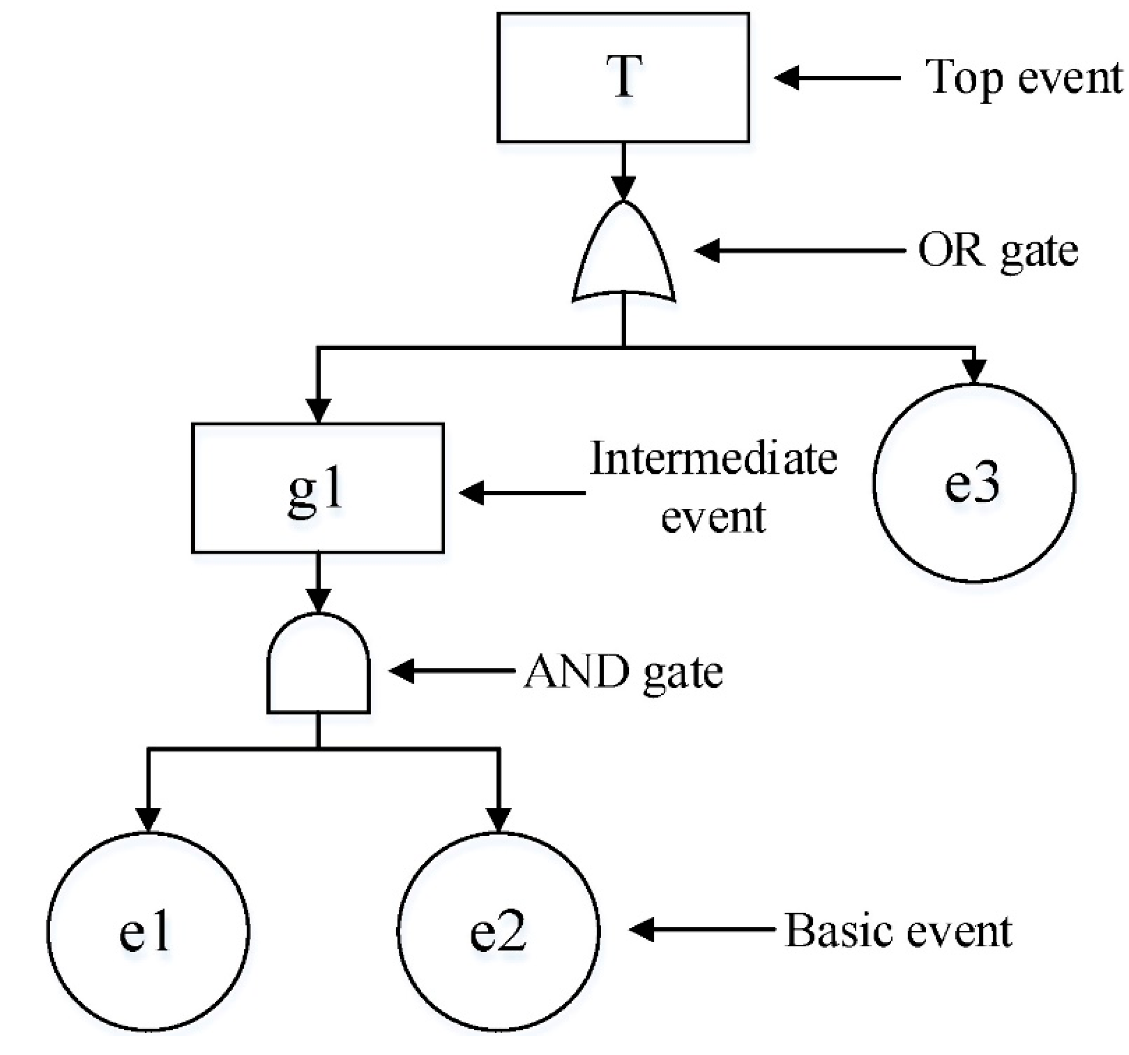
3.2. Fault Tree Analysis
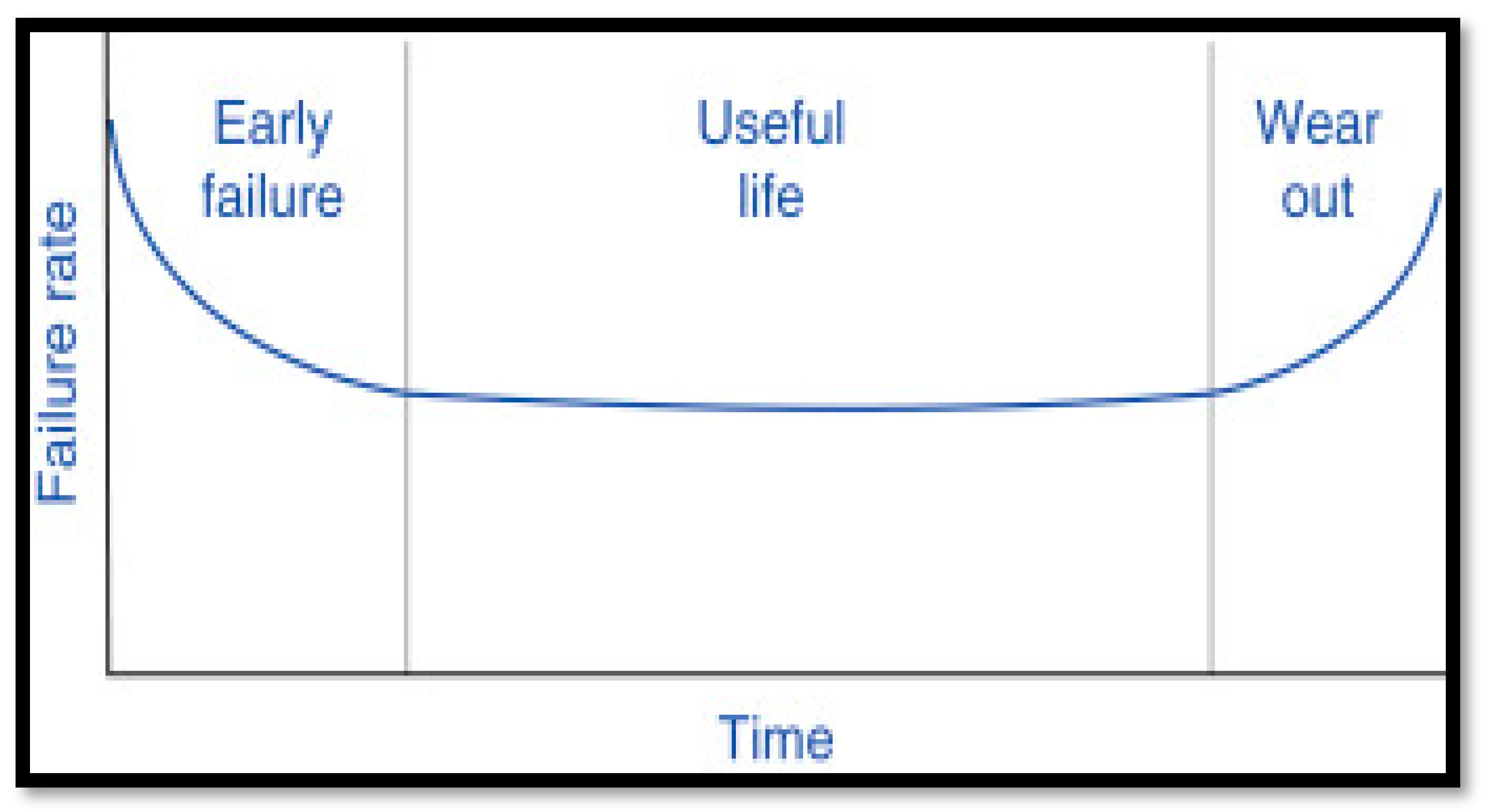
3.3. Probability Distributions and NHPP Models
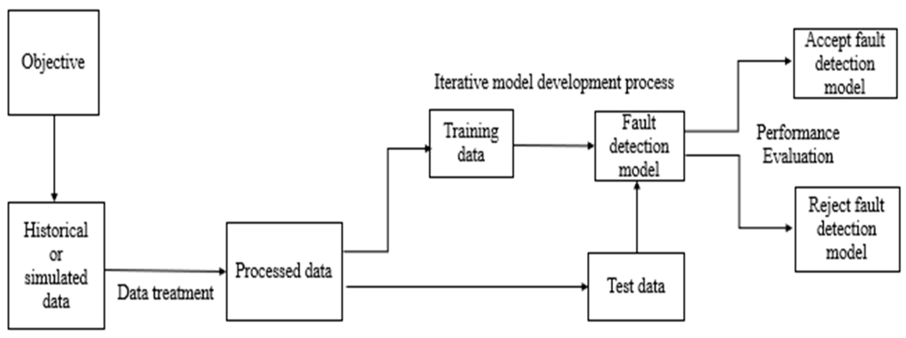
4. Machine Learning Applications in Failure Predictions and Reliability Estimations
- Supervised learning: The algorithm creates a function that maps inputs to outputs. Output variables are known. The classification problem is a common supervised learning challenge in which the learner must learn (or estimate the behaviors of) a function that maps a vector into one of many classes by studying multiple input-output samples of the function.
- Unsupervised learning: There is no target or outcome variable to predict/estimate in this method. It is used for clustering populations in different groups and when there is a lack of sufficiently labelled data [74].
- Semi-supervised learning: Combines both labelled and unlabeled examples to generate an appropriate function or classifier [75]
- Reinforcement learning: The machine is taught to make a certain decision using this algorithm. It works like this: the machine is placed in an environment where it would constantly train itself through trial and error. This system learns from its previous experiences and seeks to capture as much information as possible to make accurate decisions [74].
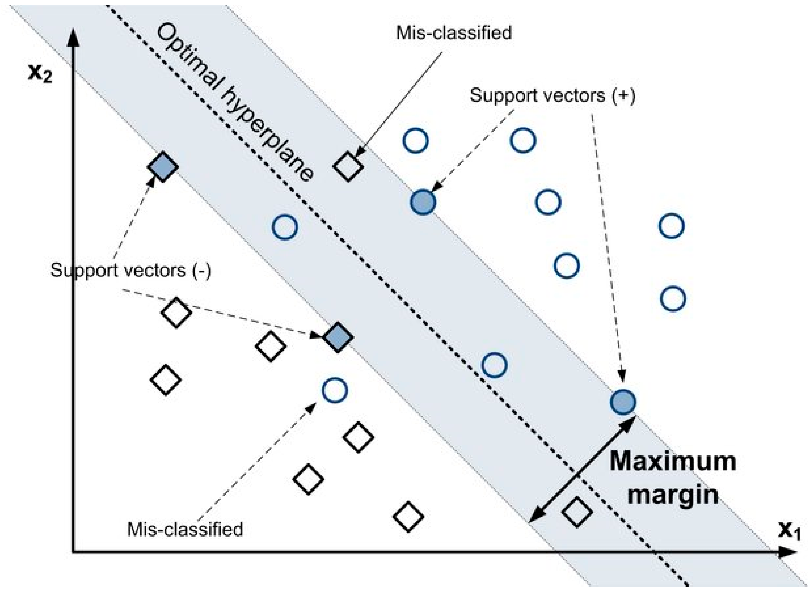
4.1. Support Vector Machine (SVM)
4.2. The k-Nearest Neighbors KNN
4.3. Naïve Bayes Classifier
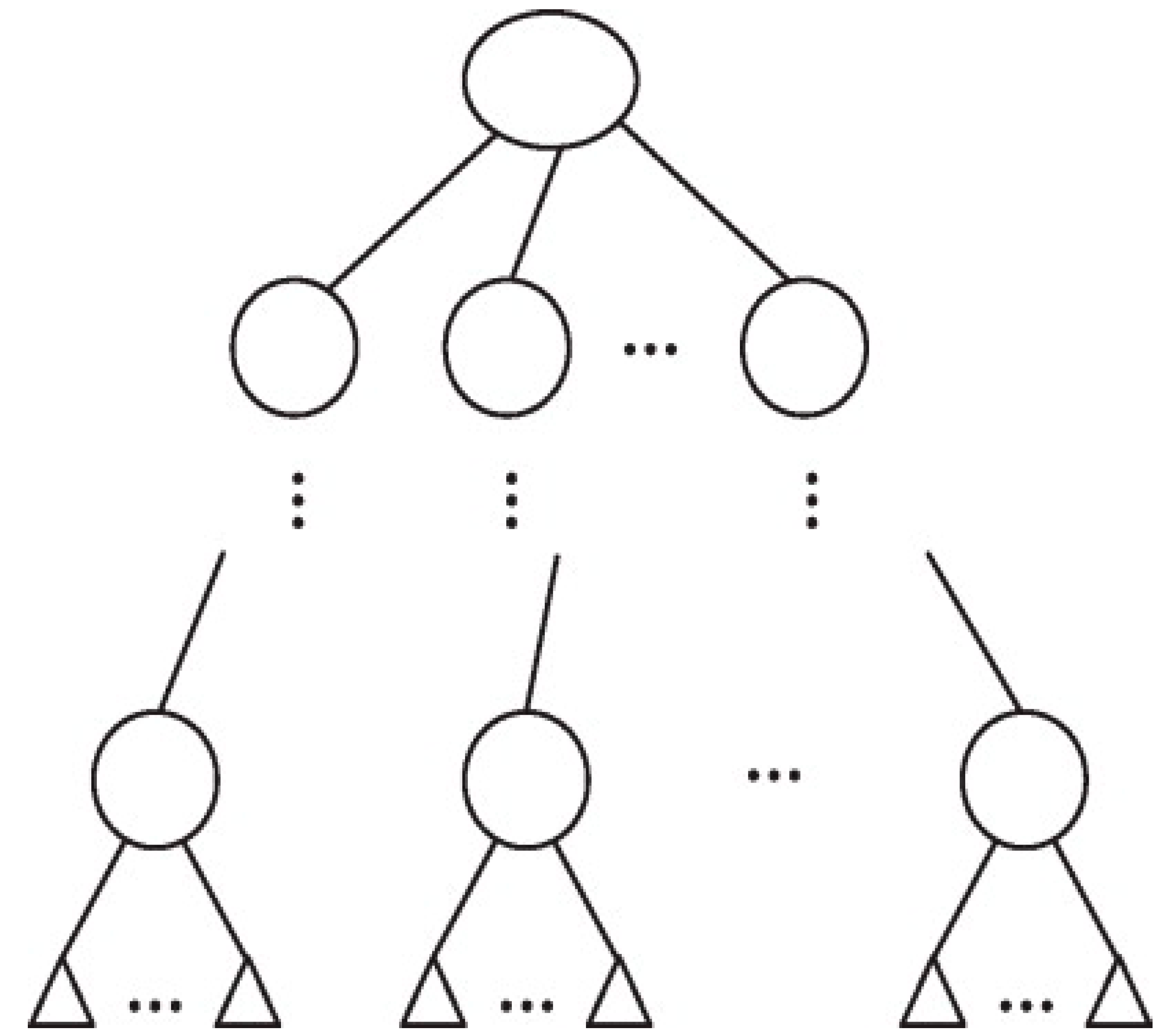
4.4. Decision Tree
4.5. Logistic Regression
4.6. K-Means Algorithm
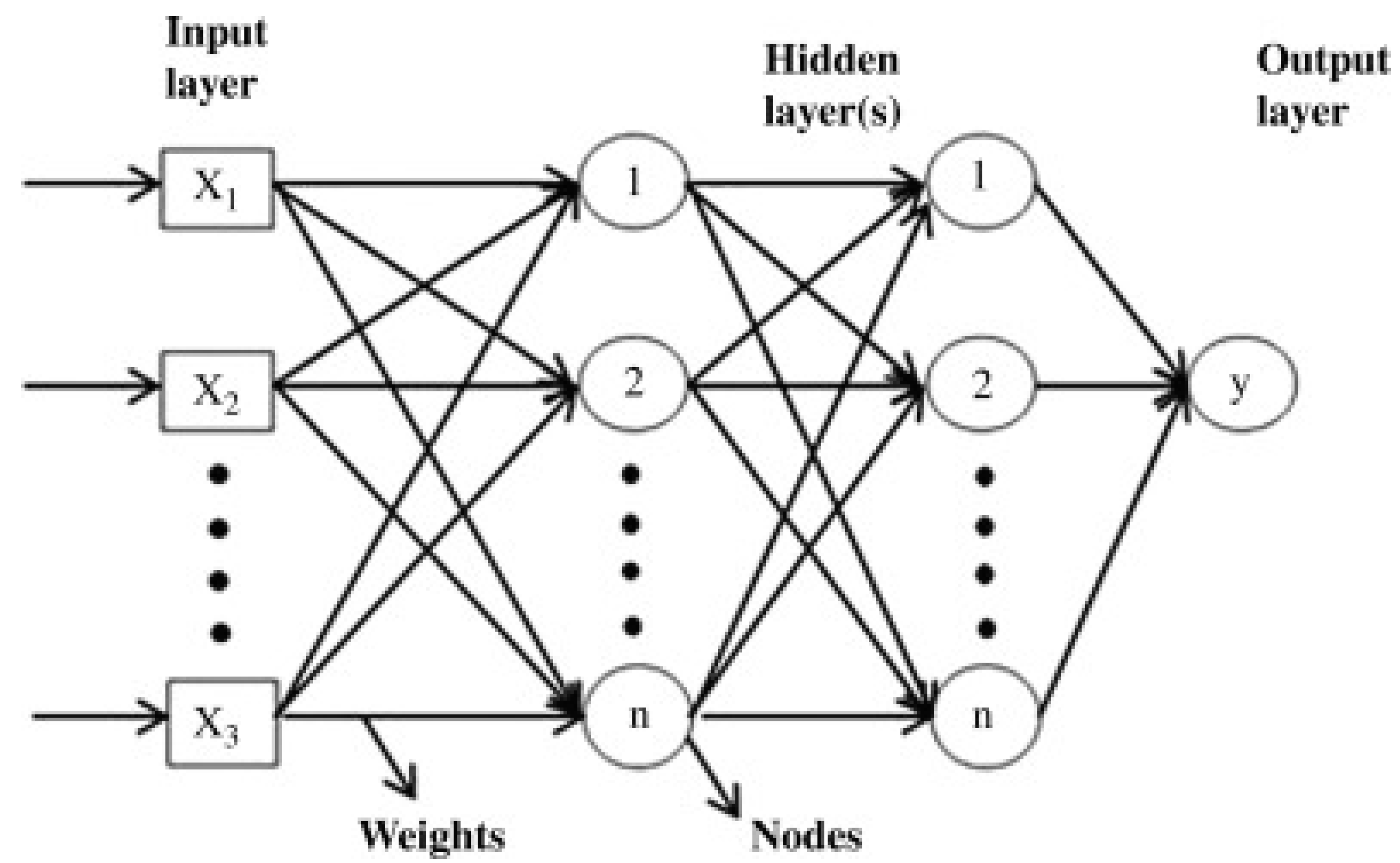
4.7. The Neural Network ANN
5. Discussions and Conclusions
Author Contributions
Funding
Institutional Review Board Statement
Informed Consent Statement
Conflicts of Interest
References
- Dhillon, B.S. Mining Equipment Reliability, Maintainability, and Safety; Springer: London, UK, 2008. [Google Scholar]
- Carlo, F.D. Reliability and Maintainability in Operations Management; Massimiliano, S., Ed.; InTech: London, UK, 2013. [Google Scholar]
- Mencik, J. Reliability of Systems. In Concise Reliability for Engineers; Mencik, J., Ed.; InTech: London, UK, 2016; p. 214. [Google Scholar]
- Kumar, U.; Klefsjo, B. Reliability analysis of hydraulic systems of LHD machines using the power law process model. Reliab. Eng. Syst. Saf. 1992, 35, 217–224. [Google Scholar] [CrossRef]
- Troy, D. The Importance of Efficient Mining Equipment. Available online: https://industrytoday.com/importance-efficient-mining-equipment/ (accessed on 12 February 2018).
- Amy, H. What Is Equipment Reliability and How Do You Improve It? Available online: https://nonstopreliability.com/equipment-reliability/ (accessed on 15 October 2020).
- Blischke, W.; Murthy, D. Case Studies in Reliability and Maintenance; Wiley: Hoboken, NJ, USA, 2003. [Google Scholar]
- Kobbacy, K.; Murthy, D. Complex Systems Maintenance Handbook; Springer: London, UK, 2008; pp. 417–436. [Google Scholar]
- Christiansen, B. Exploring Biggest Maintenance Challenges in the Mining Industry. Available online: https://www.mining.com/web/exploring-biggest-maintenance-challenges-mining-industry/#:~:text=Mining%20equipment%20maintenance%20is%20so,equipment%20maintenance%20and%20repair%20alone.&text=Deploying%20such%20technology%20in%20maintenance,can%20significant (accessed on 30 July 2018).
- Norris, G. The True Cost of Unplanned Equipment Downtime. Available online: https://www.forconstructionpros.com/equipment-management/article/21104195/the-true-cost-of-unplanned-equipment-downtime (accessed on 3 December 2019).
- Kumar, U. Reliability Analysis of Load-Haul-Dump Machines. Ph.D. Thesis, Lulea tekniska universitet, Lulea, Sweden, 1990. [Google Scholar]
- Provencher, M. A Guide to Predictive Maintenance for the Smart Mine. Available online: https://www.mining.com/a-guide-to-predictive-maintenance-for-the-smart-mine/ (accessed on 16 April 2020).
- Sellathamby, C.; Moore, B.; Slupsky, S. Increased Productivity by Condition-Based Maintenance Using Wireless Strain Measurement System. In Proceedings of the Canadian Institute of Mining (CIM) MEMO Conference, Sudbury, ON, Canada, 24–27 October 2010. [Google Scholar]
- Coetzee, J.L. Maintenance; Trafford Publishing: Bloomington, IN, USA, 2004. [Google Scholar]
- Correa, J.C.A.J.; Guzman, A.A. Mechanical Vibrations and Condition Monitoring; Academic Press: Cambridge, MA, USA, 2020. [Google Scholar]
- Kendon, P. How Well Do You Understand the Key Metrics for Reliability and Maintenance? Available online: https://www.prometheusgroup.com/posts/how-well-do-you-understand-the-key-metrics-for-reliability-and-maintenance (accessed on 24 September 2019).
- Alla, H.R.; Hall, R.; Apel, D. Performance evaluation of near real-time condition monitoring in haul trucks. Int. J. Min. Sci. Technol. 2020, 30, 909–915. [Google Scholar] [CrossRef]
- Ambrose, D.H. Research on Reliability of Mine Equipment: A Status Report; Department of the Interior, Bureau of Mines: Washington, DC, USA, 1985.
- Singh, B.P.; Tiari, S. Application of reliability and availability to underground mine transport. J. Mines Met. Fuels (India) 1984, 32, 23–30. [Google Scholar]
- Zakharchenko, A.I.; Leusenko, Y.A. A comprehensive approach to solution of the problem of improving the quality of mine equipment. Ugol’Ukr (Ukr. SSR) 1980, 7, 16–17. [Google Scholar]
- Viray, F.L. Coal Mine Productivity Assessment as Influenced by Equipment Reliability and Availability; ProQuest Dissertations Publishing: Ann Arbor, MI, USA, 1982; p. 338. [Google Scholar]
- Dietl, W. Optimization of the structure of surface mine equipment systems. Hebezeuge Foerdermittel 1985, 25, 357–361. [Google Scholar]
- Kumar, U.; Klefsjo, B.; Granholm, S. Reliability Investigation for a Fleet of Load Haul Dump Machines in a Swedish Mine. Reliab. Eng. Syst. Saf. 1989, 26, 341–361. [Google Scholar] [CrossRef]
- Klefsjo, B.; Kumar, U. Goodness-of-fit tests for the power-law process based on the TTT-plot. IEEE Trans. Reliab. 1992, 41, 593–598. [Google Scholar] [CrossRef]
- Soljacic, V.; Kosic, M. Reliability diagnostics of electronic equipment. Measurement 1990, 8, 141–144. [Google Scholar] [CrossRef]
- Stanek, E.; Venkata, S. Mine power system reliability. IEEE Trans. Ind. Appl. 1988, 24, 827–838. [Google Scholar] [CrossRef]
- Collins, E.W. Safety evaluation of coal mine power systems. In Proceedings of the Annual Reliability and Maintainability Symposium, Philadelphia, PA, USA, 27 January 1987; Sandia National Labs.: Albuquerque, NM, USA, 1987. [Google Scholar]
- Samanta, B.; Sarkar, B.; Mukherjee, S.K. Reliability assessment of hydraulic shovel system using fault trees. Min. Technol. Trans. Inst. Min. Metall. Sect. A 2002, 111, 129–135. [Google Scholar] [CrossRef]
- Barabady, J. Reliability and maintainability analysis of crushing plants in Jajarm bauxite mine of Iran. In Annual Symposium on Reliability and Maintainability (RAMS); IEEE: Alexandria, VA, USA, 2005. [Google Scholar]
- Samanta, B.; Sarkar, B.; Mukherjee, S.K. Mineral Resources Engineering; Imperial College Press: London, UK, 2001; pp. 219–231. [Google Scholar] [CrossRef]
- Coetzee, J.L. The role of NHPP models in the practical analysis of maintenance failure data. Reliab. Eng. Syst. Saf. 1997, 56, 161–168. [Google Scholar] [CrossRef]
- Roy, S.K.; Bhattacharyya, M.M.; Naikan, V.N. Maintainability and reliability analysis of a fleet of shovels. Min. Technol. Trans. Inst. Min. Metall. Sect. A 2001, 110, 163–171. [Google Scholar] [CrossRef]
- Vagenas, N.; Runciman, N.; Clément, S.R. A methodology for maintenance analysis of mining equipment. Int. J. Surf. Min. Reclam. Environ. 1997, 11, 33–40. [Google Scholar] [CrossRef]
- Vagenas, N.; Nuziale, T. Genetic Algorithm for reliability assessment of mining equipment. J. Qual. Maint. Eng. 2001, 7, 302–311. [Google Scholar] [CrossRef]
- Hall, R.A.; Daneshmend, L.K. Reliability Modelling of Surface Mining Equipment: Data Gathering and Analysis Methodologies. Int. J. Surf. Min. 2003, 17, 139–155. [Google Scholar] [CrossRef]
- Ascher, H.; Feingold, H. Repairable Systems Reliability: Modeling, Inference, Misconceptions and Their Causes; Marcel Dekker, Inc.: New York, NY, USA, 1984. [Google Scholar]
- Barlow, R.E. Analysis of Retrospective Failure Data Using Computer Graphics. In Proceedings of the Annual Reliability and Maintainability Symposium, Los Angeles, CA, USA, 17–19 January 1978. [Google Scholar]
- Crow, L.H. Reliability Analysis of Complex Repairable Systems. In Reliability and Biometry; Proschan, F., Serfling, R.J., Eds.; SIAM: Philadelphia, PA, USA, 1974. [Google Scholar]
- Ahmadi, S.; Hajihassani, M.; Moosazadeh, S.; Moomivand, H. An Overview of the Reliability Analysis Methods of Tunneling Equipment. CrossMark 2020, 14, 218–219. [Google Scholar] [CrossRef]
- Klefsjo, B. TTT-plotting—A tool for both theoretical and practical problems. J. Stat. Plan. Inference 1991, 29, 99–110. [Google Scholar] [CrossRef]
- Rao, K.R.; Prasad, P.V. Graphical methods for reliability of repairable equipment and maintenance planning. In Proceedings of the Annual Symposium on Reliability and Maintainability (RAMS), Philadelphia, PA, USA, 22–25 January 2001; pp. 123–128. [Google Scholar]
- Kumar, R.; Vardhan, A.; Kishorilal, D.B.; Kumar, A. Reliability analysis of a hydraulic shovel used in open pit coal mines. J. Mines Met. Fuels 2018, 66, 472–477. [Google Scholar]
- Sinha, R.S.; Mukhopadhyay, A.K. Reliability centered maintenance of cone crusher: A case study. Int. J. Syst. Assur. Eng. Manag. 2015, 6, 32–35. [Google Scholar] [CrossRef]
- Ruijters, E.; Stoelinga, M. Fault Tree Analysis: A survey of the state-of-the-art in modeling, analysis and tools. Comput. Sci. Rev. 2015, 15–16, 29–62. [Google Scholar] [CrossRef]
- Yong, B.; Qiang, B. Subsea Engineering Handbook; Gulf Professional Publishing: Oxford, UK, 2018. [Google Scholar]
- Singh, R. Pipeline Integrity Handbook; Gulf Professional Publishing: Oxford, UK, 2017. [Google Scholar]
- Gharahasanlou, A.N.; Mokhtarei, A.; Khodayarei, A.; Ataei, M. Fault tree analysis of failure cause of crushing plant and mixing bed hall at Khoy cement factory in Iran. Case Stud. Eng. Fail. Anal. 2014, 2, 33–38. [Google Scholar] [CrossRef] [PubMed]
- Kang, J.; Sun, L.; Soares, C.G. Fault Tree Analysis of floating offshore wind turbines. Renew. Energy 2019, 133, 1455–1467. [Google Scholar] [CrossRef]
- Tuncay, D.; Nuray, D. Reliability analysis of a dragline using fault tree analysis. Bilimsel Madencilik Derg. 2017, 56, 55–64. [Google Scholar] [CrossRef] [Green Version]
- Patil, R.B.; AMhamane, D.; Kothavale, P.B.; SKothavale, B. Fault Tree Analysis: A Case Study from Machine Tool Industry. In Proceedings of the An International Conference on Tribology, TRIBOINDIA-2018, Mumbai, India, 13–15 December 2018. [Google Scholar]
- Iyomi, E.P.; Ogunmilua, O.O.; Guimaraes, I.M. Managing the Integrity of Mine Cage Conveyance. Int. J. Eng. Res. Technol. (IJERT) 2021, 10, 743–747. [Google Scholar] [CrossRef]
- Relkar, A.S. Risk Analysis of Equipment Failure through Failure Mode and Effect Analysis and Fault Tree Analysis. J. Fail. Anal. Prev. 2021, 21, 793–805. [Google Scholar] [CrossRef]
- Li, S.; Yang, Z.; Tian, H.; Chen, C.; Zhu, Y.; Deng, F.; Lu, S. Failure Analysis for Hydraulic System of Heavy-Duty Machine. Appl. Sci. 2021, 11, 1249. [Google Scholar] [CrossRef]
- Jiang, G.-J.; Li, Z.-Y.; Qiao, G.; Chen, H.-X.; Li, H.-B.; Sun, H.-H. Reliability Analysis of Dynamic Fault Tree Based on BinaryDecision Diagrams for Explosive Vehicle. Math. Probl. Eng. 2021, 2021, 5559475. [Google Scholar] [CrossRef]
- Kabir, S. An overview of fault tree analysis and its application in model based dependability analysis. Expert Syst. Appl. 2017, 77, 114–135. [Google Scholar] [CrossRef]
- Yin, T.; Liu, Q.; Tang, X.; Zhao, Y.; Yang, J.; Wu, M. Fault Diagnosis of Roadheader Based on Dynamic Fault Tree. In Proceedings of the 3rd International Conference on Engineering Technology and Application, Singapore, 20–21 January 2017; p. 2016. [Google Scholar]
- Wang, W.H.; Zhang, D.K.; Cheng, G.; Shen, L.H. The Dynamic Fault Tree Analysis of Not-Cutting Failure for MG550/1220 Electrical Haulage Shearer. Appl. Mech. Mater. 2011, 130–134, 646–649. [Google Scholar] [CrossRef]
- Geitner, F.K.; Bloch, H.P. Practical Machinery Management for Process Plants; Gulf Professional Publishing: Oxford, UK, 2006; Volume 5. [Google Scholar]
- Coolen, F. Parametric probability distributions in reliability. In Quantitative Risk Analysis and Assessment; Melnick, E.L., Everitt, B.S., Eds.; Wiley: West Sussex, UK, 2008. [Google Scholar]
- Zuo, X.; Yu, X.R.; Yue, Y.L.; Yin, F.; Zhu, C.L. Reliability Study of Parameter Uncertainty Based on Time-Varying Failure Rates with an Application to Subsea Oil and Gas Production Emergency Shutdown Systems. Processes 2021, 9, 2214. [Google Scholar]
- Kumar, N.S.; Choudhary, R.P.; Murthy, C. Reliability based analysis of probability density function and failure rate of the shovel-dumper system in a surface coal mine. Modeling Earth Syst. Environ. 2020, 7, 1727–1738. [Google Scholar] [CrossRef]
- Balaraju, J.; Raj, M.G.; Murthy, C. Estimation of reliability-based maintenance time intervals of Load-Haul Dumper in an underground coal mine. J. Min. Environ. 2018, 9, 761–771. [Google Scholar]
- Barabady, J.; Kumar, U. Reliability analysis of mining equipment: A case study of a crushing plant at Jajarm Bauxite Mine in Iran. Reliab. Eng. Syst. Saf. 2008, 93, 647–653. [Google Scholar] [CrossRef]
- Taherı, M.; Bazzazı, A.A. Reliability Analysis of Loader Equipment: A Case Study of a Galcheshmeh. J. Undergr. Resour. 2016, 37–46. Available online: https://dergipark.org.tr/en/pub/mtb/issue/32053/354893 (accessed on 3 March 2022).
- Bala, R.J.; Govinda, R.; Murthy, C. Reliability analysis and failure rate evaluation of load haul dump machines using Weibull. Math. Model. Eng. Probl. 2018, 5, 116–122. [Google Scholar] [CrossRef]
- Waghmode, L.Y.; Patil, R.B. Reliability analysis and life cycle cost optimization: A case study from Indian industry. Int. J. Qual. Reliab. Manag. 2016, 33, 414–429. [Google Scholar] [CrossRef]
- Vashistha, S.; Agrawal, A.K.; Siddiqui, M.A.; Chattopadhyaya, S. Reliability and Maintainability Analysis of LHD Loader at Saoner Mines, Nagpur, India. IOP Conf. Ser. Mater. Sci. Eng. 2019, 691, 012013. [Google Scholar] [CrossRef]
- Rahimdel, M.J.; Ataei, M.; Khalokakaei, R.; Hoseinie, S.H. Maintenance plan for a fleet of rotary drill rigs. Arch. Min. Sci. 2014, 59, 441–453. [Google Scholar]
- Hoseinie, S.H.; Ataei, M.; Khalokakaie, R.; Ghodrati, B.; Kumar, U. Reliability analysis of the cable system of drum shearer using the power law process model. Int. J. Min. Reclam. Environ. 2012, 26, 309–323. [Google Scholar] [CrossRef]
- Mouli, C.; Chamarthi, S.; Chandra, G.; Kumar, V. Reliability Modeling and Performance Analysis of Dumper Systems in Mining by KME Method. Int. J. Curr. Eng. Technol. 2014, 255–258. [Google Scholar] [CrossRef]
- Roche-Carrier, N.L.; Ngoma, G.D.; Kocaefe, Y.; Erchiqui, F. Reliability analysis of underground rock bolters using the renewal process, the non-homogeneous Poisson process and the Bayesian approach. Int. J. Qual. Reliab. Manag. 2019, 37, 223–242. [Google Scholar] [CrossRef]
- Din, I.U.; Guizani, M.; Rodrigues, J.J.; Hassan, S.; Korotaev, V.V. Machine learning in the Internet of Things: Designed techniques for smart cities. Future Gener. Comput. Syst. 2019, 100, 826–843. [Google Scholar] [CrossRef]
- Fahad, S.K.A.; Ala, M.M. Clustering, A modified K-Means Algorithm for Big Data. IJCSET 2016, 6, 129–132. [Google Scholar]
- Abdi, A. Three Types of Machine Learning Algorithms. 2016. Available online: https://www.researchgate.net/publication/310674228_Three_types_of_Machine_Learning_Algorithms (accessed on 3 March 2022).
- Ayodele, T. New Advances in Machine Learning; InTech: London, UK, 2010. [Google Scholar]
- Jordan, J. Evaluating a Machine Learning Model. Available online: https://www.jeremyjordan.me/evaluating-a-machine-learning-model/ (accessed on 21 July 2017).
- Ray, S. Understanding Support Vector Machine(SVM) Algorithm from Examples. Available online: https://www.analyticsvidhya.com/blog/2017/09/understaing-support-vector-machine-example-code/ (accessed on 13 September 2017).
- Zisserman, A. The SVM Classifier. Available online: https://www.robots.ox.ac.uk/~az/lectures/ml/lect2.pdf (accessed on 5 March 2022).
- Gordon, G. Support Vector Machines and Kernel Methods. Available online: https://www.cs.cmu.edu/~ggordon/SVMs/new-svms-and-kernels.pdf (accessed on 15 June 2004).
- Jakkula, V. Tutorial on Support Vector Machine (SVM); Report; Washington State University: Pullman, WA, USA, 2011. [Google Scholar]
- Duc, H.N.; Kamwa, I.; Dessaint, L.-A.; Cao-Duc, H. A Novel Approach for Early Detection of Impending Voltage Collapse Events Based on the Support Vector Machine. Int. Trans. Electr. Energy Syst. 2017, 27, e2375. [Google Scholar]
- Hwang, S.; Jeong, J. SVM-RBM based Predictive Maintenance Scheme for IoT-enabled Smart Factory. In Proceedings of the Thirteenth International Conference on Digital Information Management, ICDIM, Berlin, Germany, 24–26 September 2018. [Google Scholar]
- Dindarloo, S.R. Support vector machine regression analysis of LHD failures. Int. J. Min. Reclam. Environ. 2014, 30, 64–69. [Google Scholar] [CrossRef]
- Dindarloo, S.R.; Siami-Irdemoosa, E. Data mining in mining engineering: Results of classification and clustering of shovels failures data. Int. J. Min. Reclam. Environ. 2016, 31, 105–118. [Google Scholar] [CrossRef]
- Chang, Y.-W.; Wang, Y.-C.; Liu, T.; Wang, Z.-J. Fault diagnosis of a mine hoist using PCA and SVM techniques. J. China Univ. Min. Technol. 2008, 18, 327–331. [Google Scholar] [CrossRef]
- Chatterjee, S.; Dash, A.; Bandopadhyay, S. Ensemble Support Vector Machine Algorithm for Reliability Estimation of a Mining Machine. Qual. Reliab. Eng. Int. 2014, 31, 1503–1516. [Google Scholar] [CrossRef]
- Timusk, M.A.; Lipsett, M.G.; McBain, J.; Mechefske, C.K. Automated Operating Mode Classification for Online Monitoring Systems. J. Vib. Acoust. 2009, 131, 041003. [Google Scholar] [CrossRef]
- Cheng, C.-F.; Rashidi, A.; Davenport, M.A.; Anderson, D.V. Activity analysis of construction equipment using audio signals and support vector machines. Autom. Constr. 2017, 81, 240–253. [Google Scholar] [CrossRef]
- Harrison, O. Machine Learning Basics with the K-Nearest Neighbors Algorithm. Available online: https://towardsdatascience.com/machine-learning-basics-with-the-k-nearest-neighbors-algorithm-6a6e71d01761 (accessed on 10 September 2018).
- Imandoust, S.B.; Bolandraftar, M. Application of K-Nearest Neighbor (KNN) Approach for Predicting Economic Events: Theoretical Background. Int. J. Eng. Res. Appl. 2013, 3, 605–610. [Google Scholar]
- Jabbar, M.A.; Deekshatulu, B.; Chandra, P. Classification of Heart Disease Using K- Nearest Neighbor and Genetic Algorithm. Procedia Technol. 2013, 10, 85–94. [Google Scholar] [CrossRef]
- Zhang, Z. Introduction to machine learning: K-nearest neighbors. Ann. Transl. Med. 2016, 4, 218. [Google Scholar] [CrossRef] [PubMed]
- Vahed, A.T.; Ghodrati, B.; Hosseinie, S.H. Enhanced K-Nearest Neighbors Method Application in Case of Draglines Reliability Analysis. In Proceedings of the 27th International Symposium on Mine Planning and Equipment Selection, Santiago, Chile, 20–22 November 2018. [Google Scholar]
- Moosavian, A.; Ahmadi, H.; Khazaee, A.T. Comparison of two classifiers; K-nearest neighbor and artificial neural network, for fault diagnosis on a main engine journal-bearing. Shock. Vib. 2013, 20, 263–272. [Google Scholar] [CrossRef]
- Sharma, A.; Jigyasu, R.; Mathew, L.; Chatterji, S. Bearing Fault Diagnosis Using Weighted K-Nearest Neighbor. In Proceedings of the 2nd International Conference on Trends in Electronics and Informatics (ICOEI 2018), Tirunelveli, India, 11–12 May 2018. [Google Scholar]
- Pandya, D.; Upadhyay, S.; Harsha, S. Fault diagnosis of rolling element bearing with intrinsic mode function of acoustic emission data using APF-KNN. Expert Syst. Appl. 2013, 40, 4137–4145. [Google Scholar] [CrossRef]
- Wang, H.; Yu, Z.; Guo, L. Real-time Online Fault Diagnosis of Rolling Bearings Based on KNN Algorithm. J. Phys. Conf. Ser. 2020, 1486, 032019. [Google Scholar] [CrossRef]
- Zhang, N.; Wu, L.; Wang, Z.; Guan, Y. Bearing Remaining Useful Life Prediction Based on Naive Bayes and Weibull Distributions. Entropy 2018, 20, 944. [Google Scholar] [CrossRef]
- Saritas, M.M.; Yasar, A. Performance Analysis of ANN and Naive Bayes Classification Algorithm for Data Classification. Int. J. Ofintelligent Syst. Appl. Eng. 2019, 7, 88–91. [Google Scholar] [CrossRef]
- Gandhi, R. Naive Bayes Classifier. Available online: https://towardsdatascience.com/naive-bayes-classifier-81d512f50a7c (accessed on 5 May 2018).
- Prabhakaran, S. How Naive Bayes Algorithm Works? (with Example and Full Code). Available online: https://www.machinelearningplus.com/predictive-modeling/how-naive-bayes-algorithm-works-with-example-and-full-code/ (accessed on 4 November 2018).
- Zhang, N.; Wu, L.; Yang, J.; Guan, Y. Naive Bayes Bearing Fault Diagnosis Based on Enhanced Independence of Data. Sensors 2018, 18, 463. [Google Scholar] [CrossRef]
- Moghaddass, R.; Zuo, M.J. Fault Diagnosis for Multi-State Equipment with Multiple Failure. In Proceedings of the 2012 Proceedings Annual Reliability and Maintainability Symposium, IEEE, Reno, NV, USA, 23–26 January 2012. [Google Scholar]
- Yi, X.J.; Chen, Y.F.; Hou, P. Fault diagnosis of rolling element bearing using Naïve Bayes classifier. Vibroengineering Procedia 2017, 14, 64–69. [Google Scholar]
- Lu, Y. Decision tree methods: Applications for classification and prediction. Shanghai Arch. Psychiatry 2015, 27, 130. [Google Scholar]
- Rokach, L.; Maimon, O. Data Mining With Decision Trees, 2nd ed.; World Scientific Publishing Co. Pte. Ltd.: Singapore, 2015. [Google Scholar]
- Du, C.-J.; Sun, D.-W. (Eds.) Object Classification Methods. In Computer Vision Technology for Food Quality Evaluation; Elsevier Inc.: Amsterdam, The Netherlands; Academic Press: Cambridge, MA, USA, 2008; pp. 57–80. [Google Scholar]
- Kohli, M. Predicting Equipment Failure On SAP ERP Application Using Machine Learning Algorithms. Int. J. Eng. Technol. 2021, 7, 306. [Google Scholar] [CrossRef]
- Karabadji, N.E.; Seridi, H.; Khelf, I.; Laouar, L. Decision Tree Selection in an Industrial Machine Fault Diagnostics. In Proceedings of the International Conference on Model and Data Engineering, Poitiers, France, 3–5 October 2012; Springer: Berlin/Heidelberg, Germany, 2012; pp. 129–140. [Google Scholar]
- Sugumaran, V.; Muralidharan, V.; Ramachandran, K. Feature selection using Decision Tree and classification through Proximal Support Vector Machine for fault diagnostics of roller bearing. Mech. Syst. Signal Process. 2007, 21, 930–942. [Google Scholar] [CrossRef]
- Gong, Y.-S.; Li, Y. Motor Fault Diagnosis Based on Decision Tree-Bayesian Network Model. In Advances in Electronic Commerce, Web Application and Communication; Jin, D., Lin, S., Eds.; Springer: Warsaw, Poland, 2012; pp. 165–170. [Google Scholar]
- Kleinbaum, D.G.; Klein, M. Logistic Regression, 2nd ed.; Springer: New York, NY, USA, 2002. [Google Scholar]
- Hildreth, J.; Dewitt, S. Logistic Regression for Early Warning of Economic Failure. In Proceedings of the 52nd ASC Annual International Conference Proceedings, Provo, UT, USA, 13–16 April 2016. [Google Scholar]
- Bhattacharjee, P.; Dey, V.; Mandal, U.K. Risk assessment by failure mode and effects analysis (FMEA) using an interval number based logistic regression model. Saf. Sci. 2020, 132, 104967. [Google Scholar] [CrossRef]
- Ku, J.-H. A Study on Prediction Model of Equipment Failure Through Analysis of Big Data Based on RHadoop. Wirel. Pers. Commun. 2018, 98, 3163–3176. [Google Scholar] [CrossRef]
- Battifarano, M.; DeSmet, D.; Madabhushi, A.; Nabar, P. Predicting Future Machine Failure from Machine State Using Logistic Regression. Available online: https://www.researchgate.net/publication/324584543_Predicting_Future_Machine_Failure_from_Machine_State_Using_Logistic_Regression (accessed on 2 April 2022).
- Li, H.; Wang, Y.; Zhao, P.; Zhang, X.; Zhou, P. Cutting tool operational reliability prediction based on acoustic emission and logistic regression model. J. Intell. Manuf. 2015, 26, 923–931. [Google Scholar] [CrossRef]
- Na, S.; Xumin, L.; Yong, G. Research on k-means Clustering Algorithm: An Improved k-means Clustering Algorithm. In Proceedings of the 2010 Third International Symposium on Intelligent Information Technology and Security Informatics, Jinggangshan, China, 2–4 April 2010; pp. 63–67. [Google Scholar]
- Abdelhadi, A. Heuristic Approach to schedule preventive maintenance operations using K-Means methodology. Int. J. Mech. Eng. Technol. 2017, 8, 300–307. [Google Scholar]
- Riantama, R.N.; Prasanto, A.D.; Kurniati, N.; Anggrahini, D. Examining Equipment Condition Monitoring for Predictive Maintenance, A case of typical Process Industry. In Proceedings of the 5th NA International Conference on Industrial Engineering and Operations Management, Detroit, MI, USA, 10–14 August 2020. [Google Scholar]
- Park, Y.S.; Lek, S. Ecological Model Types. In Developments in Environmental Modelling; Jørgensen, S.E., Ed.; Elsevier Ltd.: Amsterdam, The Netherlands, 2016; Volume 28, pp. 1–26. [Google Scholar]
- Walczak, S.; Cerpa, N. Artificial Neural Networks. In Encyclopedia of Physical Science and Technology, 3rd ed.; Meyers, R.A., Ed.; Academic Press: Cambridge, MA, USA, 2001; pp. 609–629. [Google Scholar]
- Zhu, X.; Hou, D.; Zhou, P.; Han, Z.; Yuan, Y.; Zhou, W.; Yin, Q. Rotor fault diagnosis using a convolutional neural network with symmetrized dot pattern images. Measurement 2019, 138, 526–535. [Google Scholar] [CrossRef]
- Alguindigue, I.E.; Loskiewicz-Buczak, A.; Uhrig, R. Monitoring and diagnosis of rolling element bearings using artificial neural networks. IEEE Trans. Ind. Electron. 1993, 40, 209–217. [Google Scholar] [CrossRef]
- Sairamya, N.J.; Susmitha, L.; George, S.T.; Subathra, M.S.P. Hybrid Approach for Classification of Electroencephalographic Signals Using Time–Frequency Images with Wavelets and Texture Features. In Intelligent Data Analysis for Biomedical Applications; Academic Press: Cambridge, MA, USA, 2019; pp. 253–273. [Google Scholar]
- Jia, F.; Lei, Y.; Lin, J.; Zhou, X.; Lu, N. Deep neural networks: A promising tool for fault characteristic mining and intelligent diagnosis of rotating machinery with massive data. Mech. Syst. Signal Process. 2016, 72–73, 303–315. [Google Scholar] [CrossRef]
- Jonathan, P.; Peck, J.B. On-line condition monitoring of rotating equipment using neural networks. ISA Trans. 1994, 33, 159–164. [Google Scholar]
- Liu, R.; Yang, B.; Zio, E.; Chen, X. Artificial intelligence for fault diagnosis of rotating machinery: A review. Mech. Syst. Signal Process. 2018, 108, 33–47. [Google Scholar] [CrossRef]
- Bin, G.; Bin, G.; Gao, J.; Li, X.J.; Dhillon, B. Early fault diagnosis of rotating machinery based on wavelet packets—Empirical mode decomposition feature extraction and neural network. Mech. Syst. Signal Process. 2012, 27, 696–711. [Google Scholar] [CrossRef]
- Li, L.; Mechefske, C.K.; Li, W. Electric motor faults diagnosis using artificial neural networks. Insight Non-Destr. Test. Cond. Monit. 2004, 46, 616–621. [Google Scholar]
- Sahu, A.R.; Palei, S.K. Fault prediction of drag system using artificial neural network for prevention of dragline failure. Eng. Fail. Anal. 2020, 113, 104542. [Google Scholar] [CrossRef]
- Sanz, J.; Perera, R.; Huerta, C. Gear dynamics monitoring using discrete wavelet transformation and multi-layer perceptron neural networks. Appl. Soft Comput. 2012, 12, 2867–2878. [Google Scholar] [CrossRef] [Green Version]


| Method | Data Types | Applications | Method Distinction |
|---|---|---|---|
| Graphical methods |
|
| Works with both complete and incomplete data |
| FTA |
|
| Can work with descriptive and numerical data |
| Probability distributions and NHPP models |
|
| Data can be easily and most accurately explained |
| SVM |
|
| Can work well with small datasets |
| KNN |
|
| Can work when sub-classes and similarities in data are unknown |
| Naïve Bayes |
|
| Works on probability of previous instances |
| Decision Tree |
|
| Information gain and pruning properties |
| Logistic Regression |
|
| Estimate the importance of each feature in binary decision models |
| K-Means |
|
| Can work with the output variable unknown (unsupervised algorithm) |
| ANN |
|
| Deep learning |
Publisher’s Note: MDPI stays neutral with regard to jurisdictional claims in published maps and institutional affiliations. |
© 2022 by the authors. Licensee MDPI, Basel, Switzerland. This article is an open access article distributed under the terms and conditions of the Creative Commons Attribution (CC BY) license (https://creativecommons.org/licenses/by/4.0/).
Share and Cite
Odeyar, P.; Apel, D.B.; Hall, R.; Zon, B.; Skrzypkowski, K. A Review of Reliability and Fault Analysis Methods for Heavy Equipment and Their Components Used in Mining. Energies 2022, 15, 6263. https://doi.org/10.3390/en15176263
Odeyar P, Apel DB, Hall R, Zon B, Skrzypkowski K. A Review of Reliability and Fault Analysis Methods for Heavy Equipment and Their Components Used in Mining. Energies. 2022; 15(17):6263. https://doi.org/10.3390/en15176263
Chicago/Turabian StyleOdeyar, Prerita, Derek B. Apel, Robert Hall, Brett Zon, and Krzysztof Skrzypkowski. 2022. "A Review of Reliability and Fault Analysis Methods for Heavy Equipment and Their Components Used in Mining" Energies 15, no. 17: 6263. https://doi.org/10.3390/en15176263
APA StyleOdeyar, P., Apel, D. B., Hall, R., Zon, B., & Skrzypkowski, K. (2022). A Review of Reliability and Fault Analysis Methods for Heavy Equipment and Their Components Used in Mining. Energies, 15(17), 6263. https://doi.org/10.3390/en15176263