
Design of a Load Frequency Controller Based on an Optimal Neural Network

 ,
,  ,
,  and
and
Abstract
:1. Introduction
2. Related Works
3. Modelling of Load Frequency System
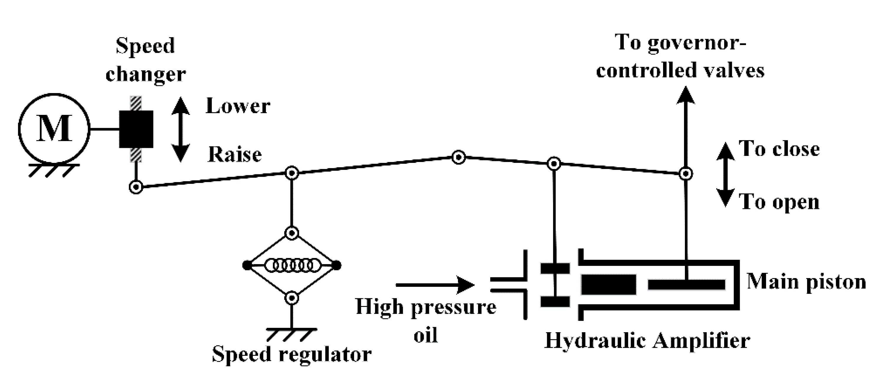
3.1. Modelling of a Single-Area PSN
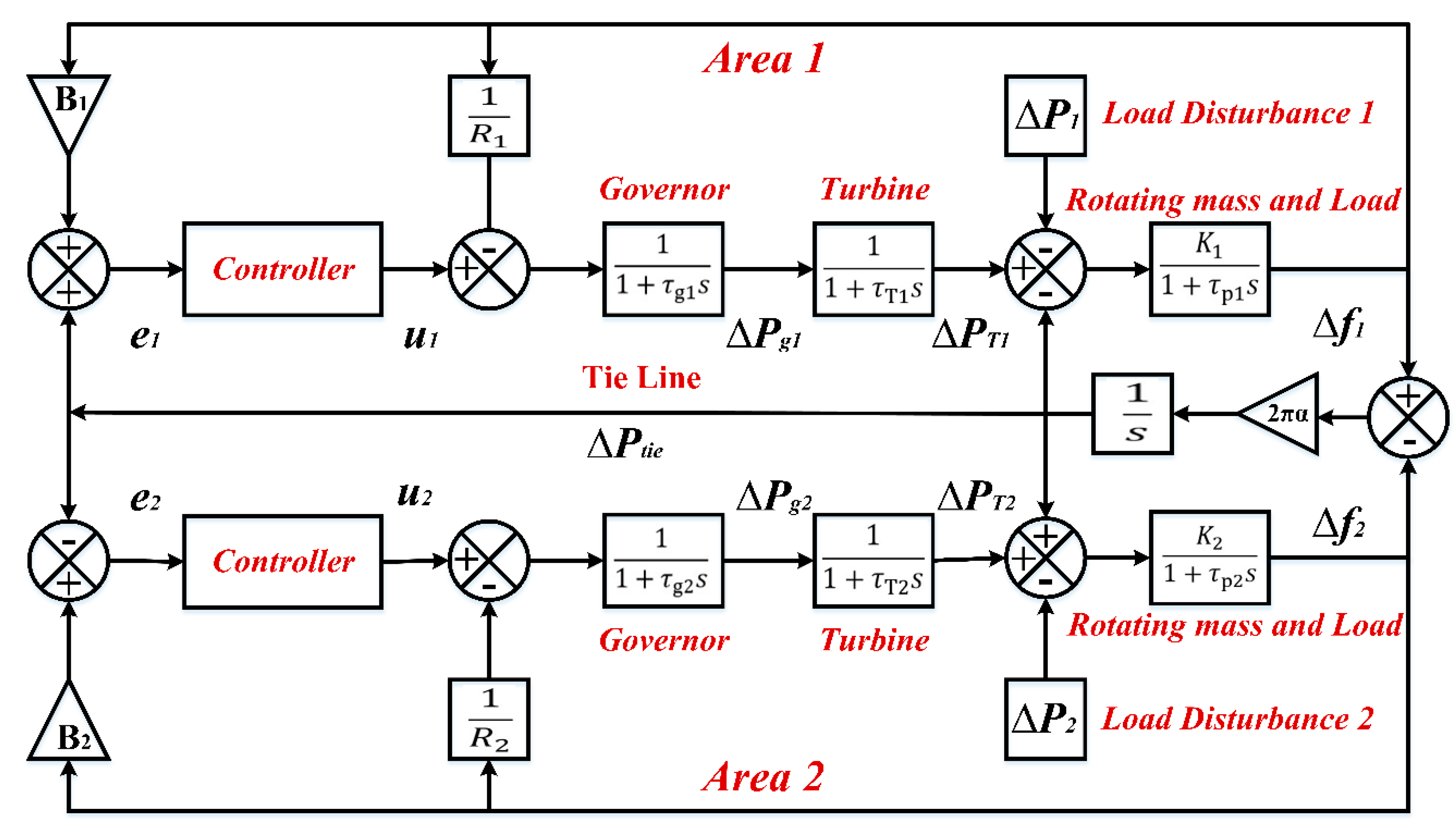
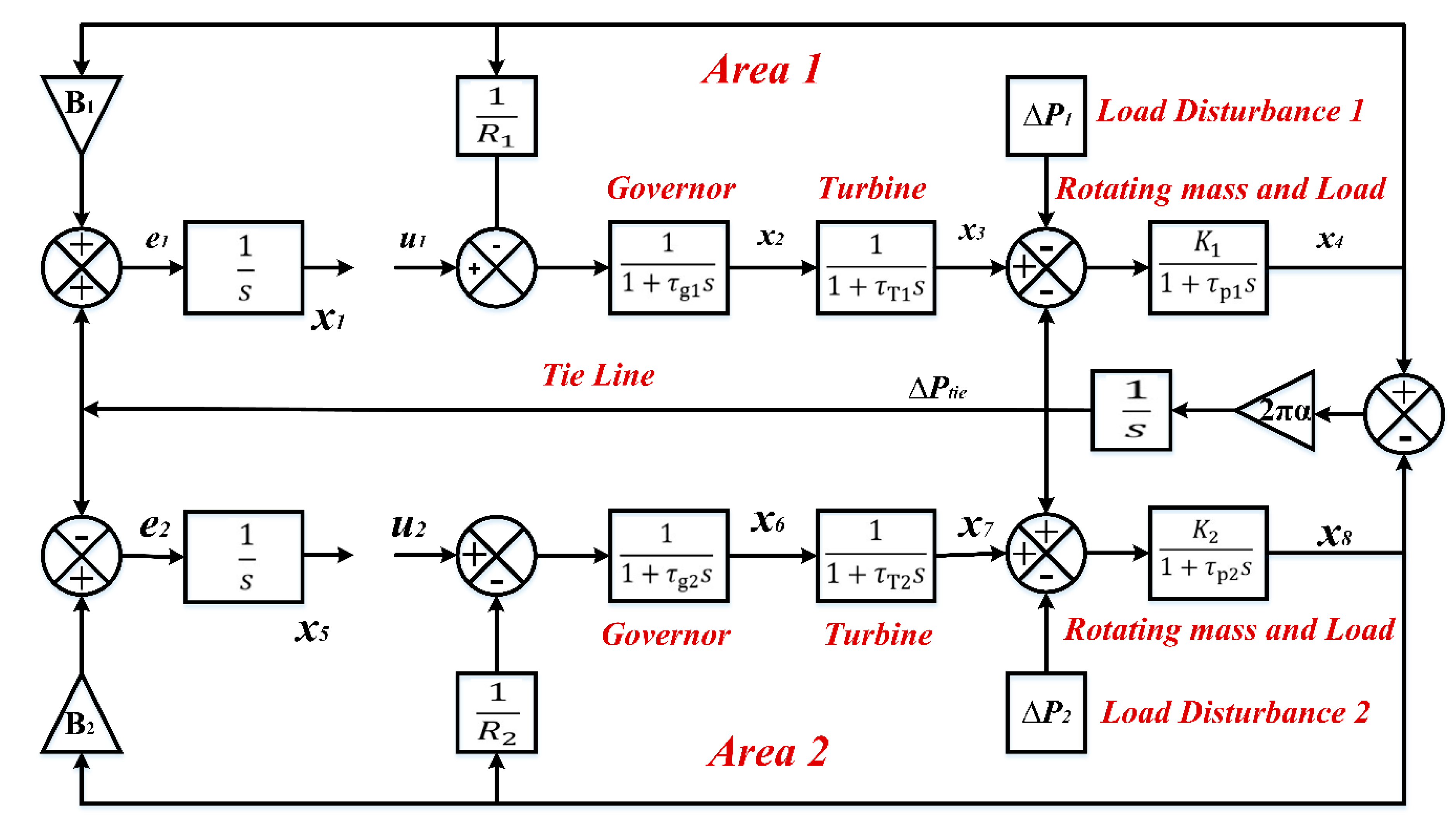
3.2. Modelling of Two-Area PSN
4. Materials and Method
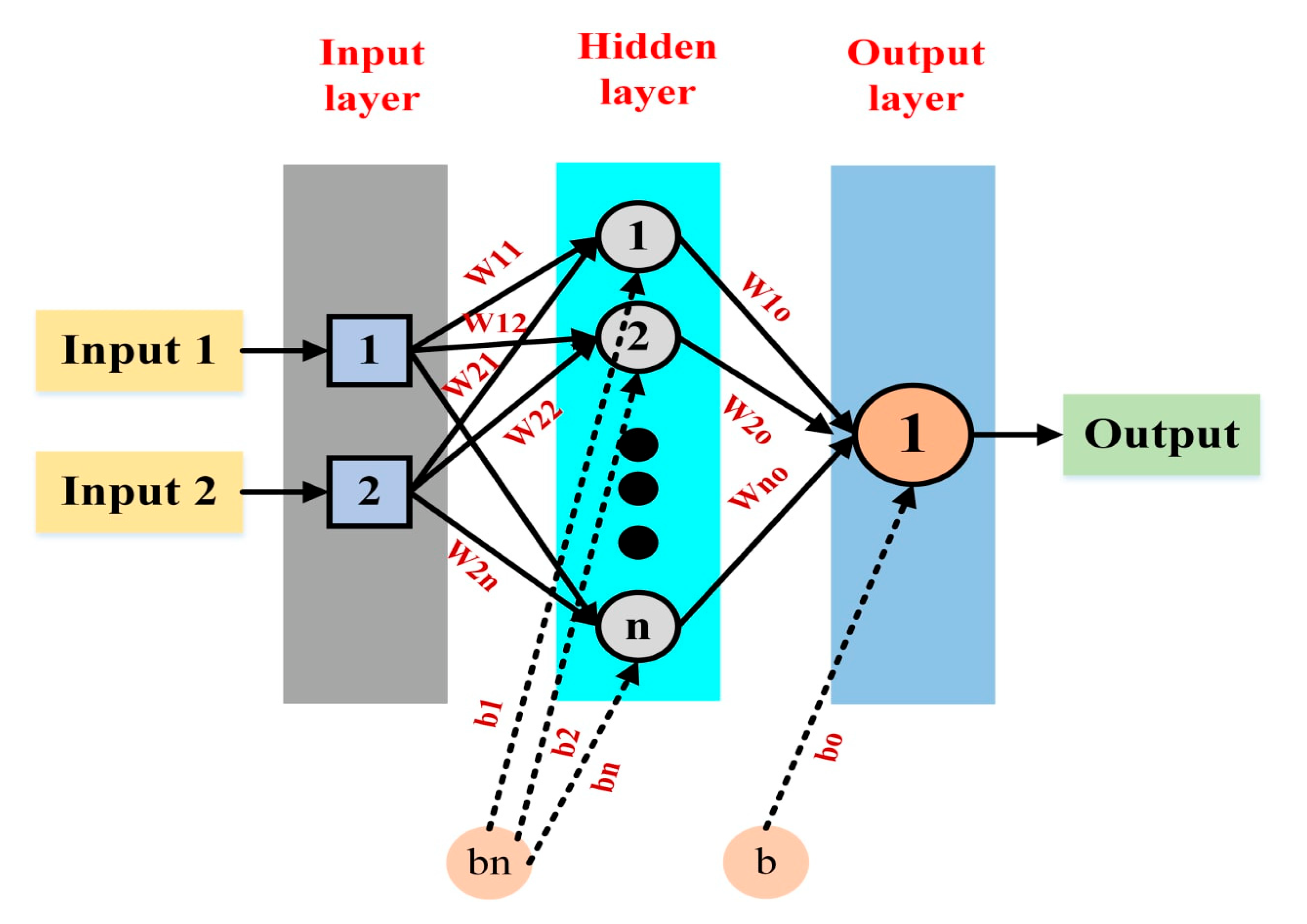
4.1. Artificial Neural Network
4.2. PSO Algorithm
- Step 1:
- It starts to search the random actual value which is chosen based on the stage of a possible case.
- Step 2:
- The former and following best values for (Pbi) and (Pli) are compared in the same state.
- Step 3:
- The best and global best solution (Gbi) are adapted and recorded to address the global value by mathematical Equations (40) and (41):where, Xi is the current position of each step, Vi is the speed search, i is the optimal value, k is the iterations, w is the inertia weighting, c1 is the cognitive coefficient, c2 is the social coefficient and r1 and r2 are the random velocity values.
- Step 4:
- The best fitness value is determined and saved.
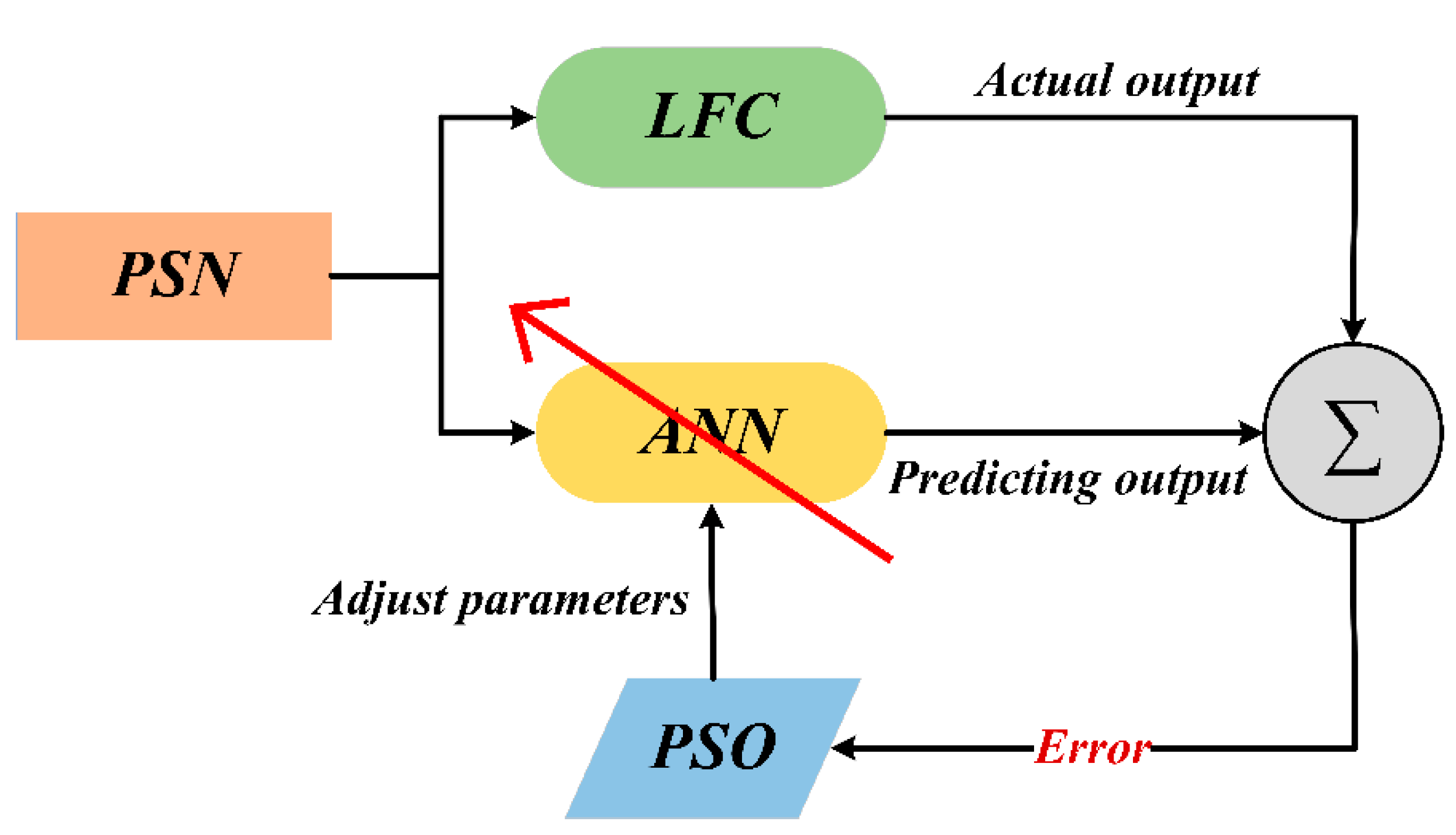
4.3. Optimal Neural Network
5. Results and Discussion
6. Conclusions
Author Contributions
Funding
Institutional Review Board Statement
Informed Consent Statement
Data Availability Statement
Acknowledgments
Conflicts of Interest
References
- Feng, W.; Xie, Y.; Luo, F.; Zhang, X.; Duan, W. Enhanced stability criteria of network-based load frequency control of power systems with time-varying delays. Energies 2021, 14, 5820. [Google Scholar] [CrossRef]
- Chen, B.Y.; Shangguan, X.C.; Jin, L.; Li, D.Y. An improved stability criterion for load frequency control of power systems with time-varying delays. Energies 2020, 13, 2101. [Google Scholar] [CrossRef]
- Ma, M.; Liu, X.; Zhang, C. LFC for multi-area interconnected power system concerning wind turbines based on DMPC. IET Gener. Transm. Distrib. 2017, 11, 2689–2696. [Google Scholar] [CrossRef]
- Yang, M.; Wang, C.; Hu, Y.; Liu, Z.; Yan, C.; He, S. Load frequency control of photovoltaic generation-integrated multi-area interconnected power systems based on double equivalent-input-disturbance controllers. Energies 2020, 13, 6103. [Google Scholar] [CrossRef]
- Ranjan, M.; Shankar, R. A literature survey on load frequency control considering renewable energy integration in power system: Recent trends and future prospects. J. Energy Storage 2022, 45, 103717. [Google Scholar] [CrossRef]
- Tan, W.; Zhang, H.; Yu, M. Decentralized load frequency control in deregulated environments. Int. J. Electr. Power Energy Syst. 2012, 41, 16–26. [Google Scholar] [CrossRef]
- Pappachen, A.; Fathima, A.P. Critical research areas on load frequency control issues in a deregulated power system: A state-of-the-art-of-review. Renew. Sustain. Energy Rev. 2017, 72, 163–177. [Google Scholar] [CrossRef]
- Alhelou, H.H.; Hamedani-Golshan, M.E.; Zamani, R.; Heydarian-Forushani, E.; Siano, P. Challenges and opportunities of load frequency control in conventional, modern and future smart power systems: A comprehensive review. Energies 2018, 11, 2497. [Google Scholar] [CrossRef]
- Kazemi, M.H.; Karrari, M.; Menhaj, M.B. Decentralized robust adaptive-output feedback controller for power system load frequency control. Electr. Eng. 2002, 84, 75–83. [Google Scholar] [CrossRef]
- Arzani, M.; Abazari, A.; Oshnoei, A.; Ghafouri, M.; Muyeen, S.M. Optimal distribution coefficients of energy resources in frequency stability of hybrid microgrids connected to the power system. Electronics 2021, 10, 1591. [Google Scholar] [CrossRef]
- Wan, X.; Wu, J. Distributed Hierarchical Control for Islanded Microgrids Based on Adjustable Power Consensus. Electronics 2022, 11, 324. [Google Scholar] [CrossRef]
- Ullah, K.; Basit, A.; Ullah, Z.; Aslam, S.; Herodotou, H. Automatic generation control strategies in conventional and modern power systems: A comprehensive overview. Energies 2021, 14, 2376. [Google Scholar] [CrossRef]
- Khooban, M.H.; Niknam, T.; Blaabjerg, F.; Davari, P.; Dragicevic, T. A robust adaptive load frequency control for micro-grids. ISA Trans. 2016, 65, 220–229. [Google Scholar] [CrossRef]
- Chen, G.; Li, Z.; Zhang, Z.; Li, S. An Improved ACO Algorithm Optimized Fuzzy PID Controller for Load Frequency Control in Multi Area Interconnected Power Systems. IEEE Access 2020, 8, 6429–6447. [Google Scholar] [CrossRef]
- Singh, V.P.; Kishor, N.; Samuel, P. Load Frequency Control with Communication Topology Changes in Smart Grid. IEEE Trans. Ind. Inform. 2016, 12, 1943–1952. [Google Scholar] [CrossRef]
- Shayeghi, H.; Shayanfar, H.A.; Jalili, A. Load frequency control strategies: A state-of-the-art survey for the researcher. Energy Convers. Manag. 2009, 50, 344–353. [Google Scholar] [CrossRef]
- Grigsby, L.L. (Ed.) Power System Stability and Control, 3rd ed.; Taylor & Francis: Abingdon, UK, 2017. [Google Scholar] [CrossRef]
- Zhong, Q.; Yang, J.; Shi, K.; Zhong, S.; Li, Z.; Sotelo, M.A. Event-Triggered H_ Load Frequency Control for Multi-Area Nonlinear Power Systems Based on Non-Fragile Proportional Integral Control Strategy. IEEE Trans. Intell. Transp. Syst. 2021, 23, 12191–12201. [Google Scholar] [CrossRef]
- Al-Majidi, S.D.; Abbod, M.F.; Al-Raweshidy, H.S. Maximum Power Point Tracking Technique based on a Neural-Fuzzy Approach for Stand-alone Photovoltaic System. In Proceedings of the 2020 55th International Universities Power Engineering Conference (UPEC), Turin, Italy, 1–4 September 2020. [Google Scholar] [CrossRef]
- Al-Majidi, S.D.; Abbod, M.F.; Al-Raweshidy, H.S. Design of an Efficient Maximum Power Point Tracker Based on ANFIS Using an Experimental Photovoltaic System Data. Electronics 2019, 8, 858. [Google Scholar] [CrossRef] [Green Version]
- Sa-ngawong, N.; Ngamroo, I. Intelligent photovoltaic farms for robust frequency stabilization in multi-area interconnected power system based on PSO-based optimal Sugeno fuzzy logic control. Renew. Energy 2015, 74, 555–567. [Google Scholar] [CrossRef]
- Al-Nussairi, M.K.; Al-Majidi, S.D.; Hussein, A.R.; Bayindir, R. Design of a Load Frequency Control based on a Fuzzy logic for Single Area Networks. In Proceedings of the 2021 10th International Conference on Renewable Energy Research and Application (ICRERA), Istanbul, Turkey, 26–29 September 2021; pp. 216–220. [Google Scholar] [CrossRef]
- Stephen, S. Load Frequency Control of Hybrid Hydro Systems using tuned PID Controller and Fuzzy Logic Controller. Int. J. Eng. Res. Technol. 2016, 5, 384–391. [Google Scholar] [CrossRef]
- Farooq, Z.; Rahman, A.; Lone, S.A. Load frequency control of multi-source electrical power system integrated with solar-thermal and electric vehicle. Int. Trans. Electr. Energy Syst. 2021, 31, 1–20. [Google Scholar] [CrossRef]
- Al-Majidi, S.D.; Abbod, M.F.; Al-Raweshidy, H.S. A particle swarm optimisation-trained feedforward neural network for predicting the maximum power point of a photovoltaic array. Eng. Appl. Artif. Intell. 2020, 92, 103688. [Google Scholar] [CrossRef]
- Wu, Y.; Feng, J. Development and Application of Artificial Neural Network. Wirel. Pers. Commun. 2018, 102, 1645–1656. [Google Scholar] [CrossRef]
- Verma, R.P.S.; Sathan, S. Intelligent automatic generation control of two-area hydrothermal power system using ANN and fuzzy logic. In Proceedings of the 2013 International Conference on Communication Systems and Network Technologies, Gwalior, India, 6–8 April 2013; pp. 552–556. [Google Scholar] [CrossRef]
- Demiroren, A.; Sengor, N.S.; Zeynelgil, H.L. Automatic generation control by using ANN technique. Electr. Power Components Syst. 2001, 29, 883–896. [Google Scholar] [CrossRef]
- Safari, A.; Babaei, F.; Farrokhifar, M. A load frequency control using a PSO-based ANN for micro-grids in the presence of electric vehicles. Int. J. Ambient Energy 2021, 42, 688–700. [Google Scholar] [CrossRef]
- Ramireddy, K.; Mudgal, Y.; Kumar, Y.V. Control of Frequency Deviation in Two-Area Interconnected Power System Using Artificial Neural Network-Based PI Controller. Soft Comput. Probl. Solving 2020, 1057, 539–553. [Google Scholar] [CrossRef]
- Kumari, K.; Shankar, G.; Kumari, S.; Gupta, S. Load frequency control using ANN-PID controller. In Proceedings of the 2011 1st International Conference on Electrical Energy Systems, ICPEICES 2016, Delhi, India, 4–6 July 2017; pp. 1–6. [Google Scholar] [CrossRef]
- Shayeghi, H.; Shayanfar, H.A. Application of ANN technique based on μ-synthesis to load frequency control of interconnected power system. Int. J. Electr. Power Energy Syst. 2006, 28, 503–511. [Google Scholar] [CrossRef]
- Chaturvedi, D.K.; Satsangi, P.S.; Kalra, P.K. Load frequency control: A generalized neural network approach. Int. J. Electr. Power Energy Syst. 1999, 21, 405–415. [Google Scholar] [CrossRef]
- Oysal, Y. A comparative study of adaptive load frequency controller designs in a power system with dynamic neural network models. Energy Convers. Manag. 2005, 46, 2656–2668. [Google Scholar] [CrossRef]
- Qian, D.; Tong, S.; Liu, H.; Liu, X. Load frequency control by neural-network-based integral sliding mode for nonlinear power systems with wind turbines. Neurocomputing 2016, 173, 875–885. [Google Scholar] [CrossRef]
- Malik, S.K.D.L.P. Analysis of Automatic Generation Control Two Area Network using ANN and Genetic Algorithm. Int. J. Sci. Res. 2013, 2, 274–278. Available online: https://www.ijsr.net/archive/v2i3/IJSRON2013535.pdf (accessed on 1 June 2022).
- Mosaad, M.I.; Salem, F. LFC based adaptive PID controller using ANN and ANFIS techniques. J. Electr. Syst. Inf. Technol. 2014, 1, 212–222. [Google Scholar] [CrossRef]
- Prasad, S.; Ansari, M.R. Frequency regulation using neural network observer based controller in power system. Control Eng. Pract. 2020, 102, 104571. [Google Scholar] [CrossRef]
- Chien, T.H.; Huang, Y.C.; Hsu, Y.Y. Neural network-based supplementary frequency controller for a DFIG wind farm. Energies 2020, 13, 5320. [Google Scholar] [CrossRef]
- Shakibjoo, A.D.; Moradzadeh, M.; Moussavi, S.Z.; Mohammadzadeh, A.; Vandevelde, L. Load frequency control for multi-area power systems: A new type-2 fuzzy approach based on Levenberg–Marquardt algorithm. ISA Trans. 2022, 121, 40–52. [Google Scholar] [CrossRef]
- Al-dunainawi, Y.; Abbod, M.F.; Jizany, A. A new MIMO ANFIS-PSO based NARMA-L2 controller for nonlinear dynamic systems. Eng. Appl. Artif. Intell. 2017, 62, 265–275. [Google Scholar] [CrossRef] [Green Version]
- Abdolrasol, M.G.M. Hussain, S.M.S.; Ustun, T.S.; Sarker, M.R.; Hannan, M.A.; Mohamed, R.; Ali, J.A.; Mekhilef, S.; Milad, A. Artificial neural networks based optimization techniques: A review. Electronics 2021, 10, 2689. [Google Scholar] [CrossRef]
- Rosa, J.P.S.; Guerra, D.J.D.; Horta, N.C.G.; Martins, R.M.F.; Lourenço, N.C.C. Overview of Artificial Neural Networks. In Using Artificial Neural Networks for Analog Integrated Circuit Design Automation; Springer: Cham, Switzerland, 2020. [Google Scholar] [CrossRef]
- Jain, A.K.; Mao, J.; Mohiuddin, K.M. Artificial neural networks: A tutorial. Computer 1996, 29, 31–44. [Google Scholar] [CrossRef]
- Basheer, I.A.; Hajmeer, M. Artificial neural networks: Fundamentals, computing, design, and application. J. Microbiol. Methods 2000, 43, 3–31. [Google Scholar] [CrossRef]
- Akkaya, R. DSP implementation of a PV system with GA-MLP-NN based MPPT controller supplying BLDC motor drive. Energy Convers. Manag. 2007, 48, 210–218. [Google Scholar] [CrossRef]
- Afs, A. A genetic algorithm optimized ANN-based MPPT algorithm for a stand-alone PV system with induction motor drive. Sol. Energy 2012, 86, 2366–2375. [Google Scholar] [CrossRef]
- Zhang, L.Ã.; Bai, Y.F. Genetic algorithm-trained radial basis function neural networks for modelling photovoltaic panels. Eng. Appl. Artif. Intell. 2005, 18, 833–844. [Google Scholar] [CrossRef]
- Hamdi, H.; Regaya, C.B.; Zaafouri, A. Real-time study of a photovoltaic system with boost converter using the PSO-RBF neural network algorithms in a MyRio controller. Sol. Energy 2019, 183, 1–16. [Google Scholar] [CrossRef]
- Marinakis, Y.; Marinaki, M.; Dounias, G. A hybrid particle swarm optimization algorithm for the vehicle routing problem. Eng. Appl. Artif. Intell. 2010, 23, 463–472. [Google Scholar] [CrossRef]
- Vasumathi, B.; Moorthi, S. Engineering Applications of Artificial Intelligence Implementation of hybrid ANN–PSO algorithm on FPGA for harmonic estimation. Eng. Appl. Artif. Intell. 2012, 25, 476–483. [Google Scholar] [CrossRef]


| Authors | Year | Connected Area | Supplied Unit | Optimised Technique |
|---|---|---|---|---|
| Chaturvedi et al. [33] | 1999 | Single and two-area | Steam turbine | Generalised neural network |
| Oysal et al. [34] | 2005 | Two-area | Steam turbine | Wavelet function |
| Shayeghi et al. [32] | 2006 | Two-area | Steam turbine | µ-synthesis |
| Demiroren et al. [28] | 2010 | Two-area | Steam turbine | Back-propagation ANN |
| Verma et al. [27] | 2013 | Two-area | Hydrothermal turbine | Standard ANN |
| Lathwal et al. [36] | 2013 | Two-area | Steam turbine | Genetic algorithm |
| Mosaad et al. [37] | 2014 | Multi-area | Steam turbine | ANFIS, ANN and GA |
| Qian et al. [35] | 2016 | Two-area | Steam turbine and wind turbine | Slide-mode |
| Kumari et al. [31] | 2017 | Two-area | Steam turbine | PID-ANN |
| Safari et al. [29] | 2019 | Two-area | diesel generation and wind turbine | Hybrid PSO-ANN |
| Prasad et al. [38] | 2020 | Two-area | Thermal turbine | Sliding mode |
| Chien et al. [39] | 2020 | Single-area | Steam and wind turbine | ANN |
| Ramireddy et al. [30] | 2021 | Multi-area | Thermal turbine | PI-ANN |
| Shakibjoo et al. [40] | 2022 | Multi-area | Thermal turbine | Multilayer ANN based on Levenberg–Marquardt algorithm |
| Parameters | Definition |
|---|---|
| Δf | The Frequency Deviation |
| ΔPtie | Tie Line Power Deviation |
| R | The Regulations of Governor |
| G | Controller Gain |
| u1and u2 | Control Inputs in Areas 1 and 2. |
| ΔPg1 and ΔPg2 | Output power Deviations at Governor |
| ΔPt1 and ΔPt2 | Output Deviations at Turbine |
| ΔP1 = D1 | Load Disturbances in Area 1 |
| ΔP2 = D2 | Load Disturbances in Area 2. |
| K1 and K2 | Constants of the PSN in Areas 1 and 2. |
| and | Time Constants of the PSN in Areas 1 and 2. |
| B1 and B2 | Tie Line Frequency Bias at Areas 1 and 2. |
| A | Synchronizing Coefficient for Tie Line |
| and | Time Constants of Governor for Areas 1 and 2. |
| and | Turbine Time Constants for Areas 1 and 2 |
| Types | Parameters |
|---|---|
| Input layer nodes of ANN | 2 |
| Output layer nodes of ANN | 1 |
| Hidden layer nodes of ANN | 23 |
| Neurons number of ANN | 93 |
| Swarm size of PSO | 50 |
| Inertia weighting of PSO | 0.75 |
| Cognitive coefficient of PSO | 1.15 |
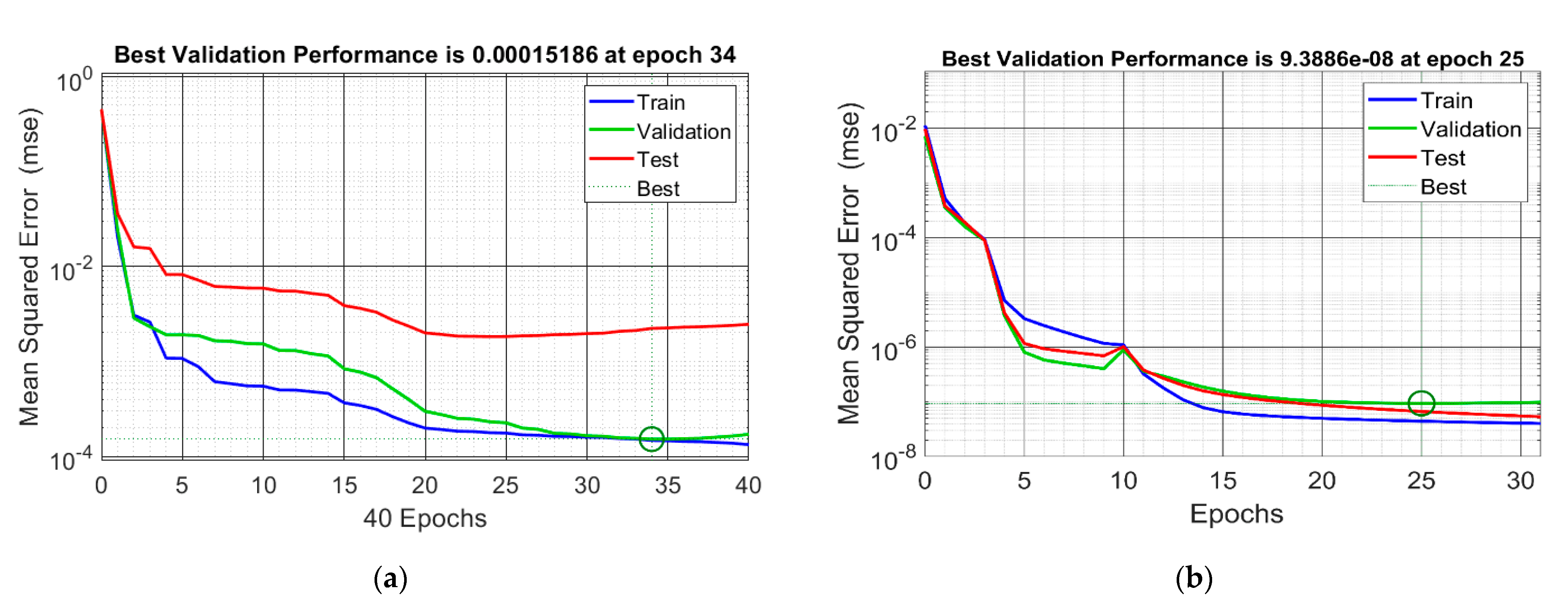
| Model | Number of Epochs | MSE |
|---|---|---|
| Optimised training | 25 | 9.3886 × 10⁻⁸ |
| Standard training | 34 | 1.518 × 10⁻⁴ |
| Training No. | ANN Topology | Number of Neurons | MSE (Average ± STD) |
|---|---|---|---|
| 1 | 2 × 10 × 1 | 41 | 0.0001518 ± 1.5 × 10⁻² |
| 2 | 2 × 20 × 1 | 81 | 0.000881 ± 1.6 × 10⁻² |
| 3 | 2 × 30 × 1 | 121 | 0.000618 ± 1.2 × 10⁻² |
| 4 | 2 × 25 × 1 | 101 | 0.000169 ± 2.5 × 10⁻² |
| 5 | 2 × 23 × 1 | 93 | 9.3886 × 10⁻⁸ ± 1.03 × 10⁻⁴ |
| Parameters | Values | ||
|---|---|---|---|
| Single-Area | Area 1 | Area 2 | |
| Base power (MVA) | 250 | 1000 | 1000 |
| The output power of the generation unit (MW) | 250 | 250 | 400 |
| The standard frequency of the system (Hz) | 60 | 60 | 60 |
| The speed regulation of the governor (pu) | 0.066 | 0.05 | 0.0625 |
| The time constant of the governor (s) | 0.2 | 0.2 s | 0.3 s |
| The time constant of the turbine (s) | 0.5 | 0.5 s | 0.6 s |
| The inertia constant of generator (s) | 5 | 5 | 4 |
| The frequency of sensitive load coefficient D | 0.6 | 0.6 | 0.9 |
| Frequency base factor B | 1 | 20 | 16.92 |
| Area 2 | Area 1 | Time | ||||
|---|---|---|---|---|---|---|
| PID | ANN | OANN | PID | ANN | OANN | |
| 0.001061 | 0.001024 | 0.000132 | 0.00145 | 0.000521 | 0.000127 | 50 |
| −0.00212 | −0.00077 | −0.00056 | −0.00388 | −0.00035 | −0.00015 | 51 |
| 0.000966 | 0.001487 | 0.000486 | 9.27 × 10⁻⁵ | 0.000103 | 7.90E−05 | 52 |
| 0.000141 | 0.000826 | −8.57 × 10⁻⁵ | 0.000856 | 0.000333 | 0.000298 | 53 |
| −0.00199 | −0.00167 | −0.00154 | 4.85 × 10⁻⁵ | 0.000108 | 2.71 × 10⁻⁵ | 54 |
| 0.000754 | 0.000679 | 0.000532 | 0.000347 | 0.000139 | 4.75 × 10⁻⁵ | 55 |
| 5.45E−05 | −0.00044 | 3.66 × 10⁻⁵ | −0.00012 | −8.58 × 10⁻⁵ | −1.00 × 10⁻⁵ | 56 |
| −0.00128 | −0.00033 | −0.00042 | 0.000112 | 0.000101 | 9.28 × 10⁻⁵ | 57 |
| −0.00068 | −0.00134 | −0.00129 | −2.57 × 10⁻⁵ | 6.92 × 10⁻⁵ | 1.01 × 10⁻⁵ | 58 |
| −0.00819 | −0.00174 | −0.00149 | −9.38 × 10⁻⁴ | −0.00015 | −0.00013 | 59 |
| 0.001967 | 0.001988 | 0.001617 | −0.00019 | −0.0002 | −0.00015 | 60 |
| −0.00066 | −0.00051 | −0.00038 | −3.61 × 10⁻⁵ | −9.54 × 10⁻⁵ | −2.94 × 10⁻⁶ | 61 |
| 0.002452 | 0.002664 | 0.002146 | 5.09 × 10⁻⁵ | 5.00 × 10⁻⁵ | 8.87 × 10⁻⁶ | 62 |
| −0.00908 | −0.00491 | −0.00415 | 1.21 × 10⁻⁵ | 5.95 × 10⁻⁵ | 9.07 × 10⁻⁶ | 63 |
| 0.009239 | 0.001811 | 0.000152 | −0.00022 | −9.25 × 10⁻⁵ | −1.43 × 10⁻⁵ | 64 |
| −0.00114 | −0.00089 | −0.00014 | −0.00013 | 2.85 × 10⁻⁵ | −1.73 × 10⁻⁵ | 65 |
| −0.0092 | −0.00124 | −0.00085 | −0.00018 | −0.00019 | −9.52 × 10⁻⁵ | 66 |
| −0.00068 | 0.000161 | −0.00014 | 5.84 × 10⁻⁵ | 4.98 × 10⁻⁵ | 4.84 × 10⁻⁵ | 67 |
| 0.000527 | −0.00068 | −0.00036 | −0.0001 | −0.00013 | −6.32 × 10⁻⁵ | 68 |
| 0.003385 | 0.002645 | 0.002278 | 0.000158 | 0.000143 | 8.62 × 10⁻⁵ | 69 |
| −0.00667 | −0.00252 | −0.00214 | 0.000322 | 0.000226 | 0.000219 | 70 |
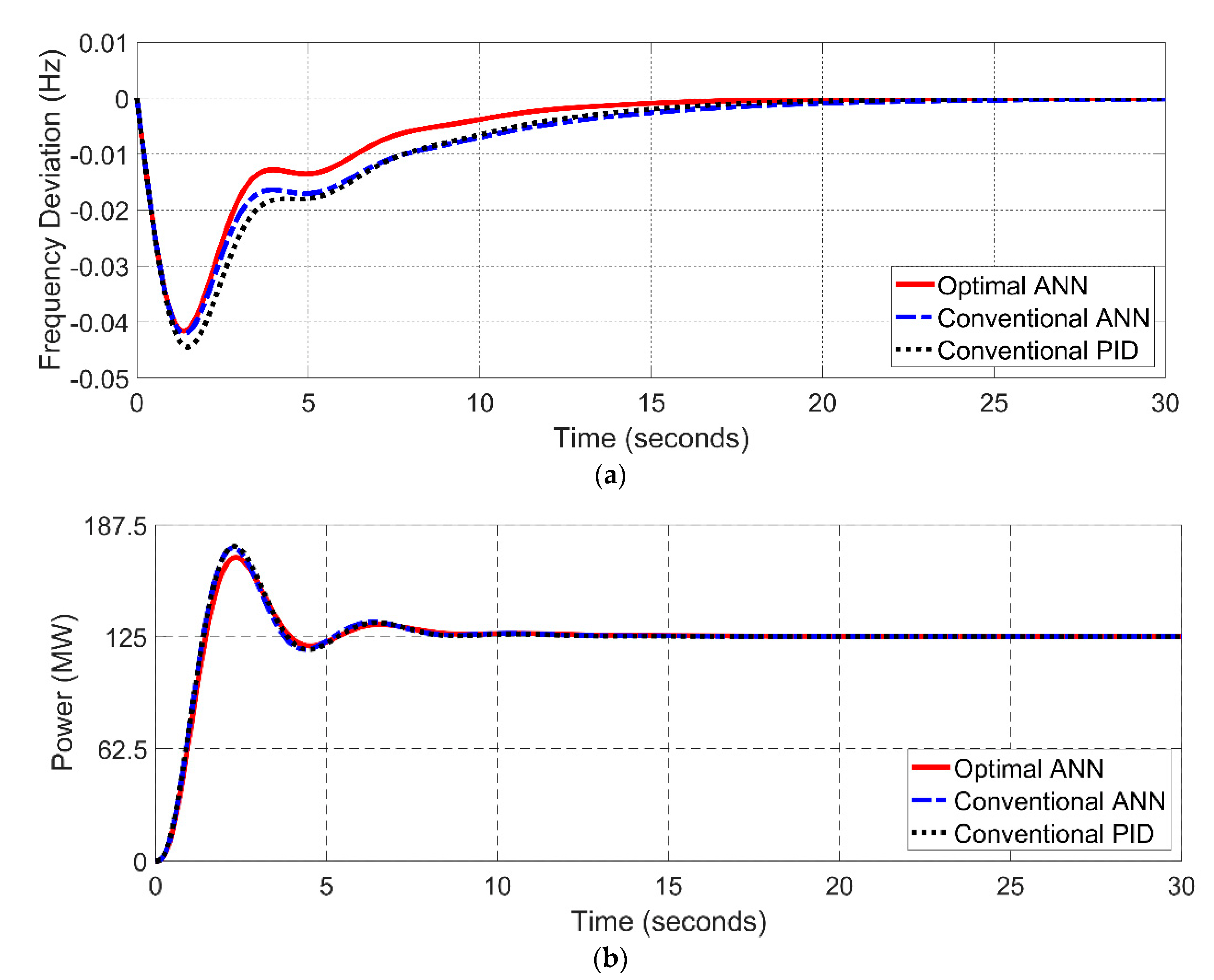
| Method | ITAE |
|---|---|
| Optimal ANN | 3.45 s |
| Conventional ANN | 7.89 s |
| Conventional PID | 10.12 s |
Publisher’s Note: MDPI stays neutral with regard to jurisdictional claims in published maps and institutional affiliations. |
© 2022 by the authors. Licensee MDPI, Basel, Switzerland. This article is an open access article distributed under the terms and conditions of the Creative Commons Attribution (CC BY) license (https://creativecommons.org/licenses/by/4.0/).
Share and Cite
Al-Majidi, S.D.; Kh. AL-Nussairi, M.; Mohammed, A.J.; Dakhil, A.M.; Abbod, M.F.; Al-Raweshidy, H.S. Design of a Load Frequency Controller Based on an Optimal Neural Network. Energies 2022, 15, 6223. https://doi.org/10.3390/en15176223
Al-Majidi SD, Kh. AL-Nussairi M, Mohammed AJ, Dakhil AM, Abbod MF, Al-Raweshidy HS. Design of a Load Frequency Controller Based on an Optimal Neural Network. Energies. 2022; 15(17):6223. https://doi.org/10.3390/en15176223
Chicago/Turabian StyleAl-Majidi, Sadeq D., Mohammed Kh. AL-Nussairi, Ali Jasim Mohammed, Adel Manaa Dakhil, Maysam F. Abbod, and Hamed S. Al-Raweshidy. 2022. "Design of a Load Frequency Controller Based on an Optimal Neural Network" Energies 15, no. 17: 6223. https://doi.org/10.3390/en15176223
APA StyleAl-Majidi, S. D., Kh. AL-Nussairi, M., Mohammed, A. J., Dakhil, A. M., Abbod, M. F., & Al-Raweshidy, H. S. (2022). Design of a Load Frequency Controller Based on an Optimal Neural Network. Energies, 15(17), 6223. https://doi.org/10.3390/en15176223