Abstract
The leakage of the tribological contact in axial piston pumps significantly impacts the pump efficiency. Leakage observations can be used to optimize the pump design and monitor the behavior of the tribological contact. However, due to assembly limitations, it is not always feasible to observe the leakage of each tribological contact individually with a flow rate sensor. This work developed a data-driven virtual flow rate sensor for monitoring the leakage of cradle bearings in axial piston pumps under different operating conditions and recess pressures. The performance of neural network, support vector regression, and Gaussian regression methods for developing the virtual flow rate sensor was systematically investigated. In addition, the effect of the number of datasets and label distribution on the performance of the virtual flow sensor were systematically studied. The findings are verified using a data-driven virtual flow rate sensor to observe the leakage. In addition, they show that the distribution of labels significantly impacts the model’s performance when using support vector regression and Gaussian regression. Neural network is relatively robust to the distribution of labeled data. Moreover, the datasets also influence model performance but are not as significant as the label distribution.
1. Introduction
Variable displacement axial piston pumps are widely used in hydraulic work machinery due to their compact structure, high power density, short fluid path, and easily adjustable stroke volume [1,2,3]. This type of pump has multiple tribological contact pairs where the gaps are filled with a fluid film. The lubricating film balances the forces on the contact surfaces and directly affects the performance of the tribological contact pairs. The lubricating film causes leakage losses and reduces the volumetric efficiency of the axial piston pump. At the same time, the friction between the contact pairs is greatly reduced, thus increasing the mechanical efficiency of the pump. Research on these tribological contact pairs in axial piston pumps has been actively conducted in recent years. Xu et al. [4] investigated the distribution of the hydro-mechanical losses in an axial piston pump over a wide range of operations. The results show that the volumetric losses are mainly from the leakage at the tribological contact pairs. Haug and Geimer [5] proposed a new approach to actively control the oil film pressure between the tribological contact pairs to achieve higher efficiency. They verified the feasibility of this new concept at the tribological contact pairs between the swashplate and cradle bearings, cylinder barrel and distributor plate, and slipper pad and swashplate. Moreover, they indicated that the method optimizes the swashplate swivel dynamics and reduces the losses at the tribological contact pairs between the swashplate and cradle bearings. Geffroy et al. [6,7] performed a geometric optimization of the tribological contact pair between the distributor plate and the cylinder barrel. The tilt angle and contact pressure between these two parts were reduced with this optimization, which positively affected the efficiency of the optimization. Liu and Geimer [8] further investigated the method proposed by Haug and Geimer [5] for hydrostatic lubrication of tribological contact pairs. They proposed a new optimization and control method for the lubrication at tribological contact pair swashplate and cradle bearing. A 90% loss at this tribological contact pair could be reduced with this method according to the simulation result. In their research, leakage value is the central part of the optimization process’s objective function and influences the optimal result significantly.
From the literature above, it can be concluded that the leakage at the tribological contact pairs is one of the performance indexes of the optimization methods and needs to be measured. In addition, the control performance of active lubrication at the tribological contact pairs can be observed and evaluated in real-time when the leakage is available. However, observation of leakage at the tribological contact pairs of series products with physical flow rate sensors is impractical due to the high cost and the considerable additional requirement for assembly space. The leakage between tribological pairs has been widely investigated using first principle modeling and can be used for internal leakage estimation. Manring [9] provided a simplified mathematical model for leakage out of the piston chamber using a classical orifice equation based on the Bernoulli equation. The discharge flow was assumed as laminar, and the relation between pressure drop and flow was assumed as linear. Ivantysynova et al. [10] introduced a novel method integrating the Reynolds equation and energy equation to simulate gap flow considering elastohydrodynamic effects. The study was utilized for the piston-cylinder contact pair. According to Li et al. [11], the nonlinear mathematical model using the Reynolds equation and energy equation could predict oil film thickness and pressure between the piston pair with high accuracy, which ensures an accurate estimation of leakage flow. The influence of different parameters such as swash plate angle, the displacement chamber pressure, and the temperature was also considered. Bergada et al. [12] utilized a novel analytical approach to produce speedy and accurate results about leakage on the barrel plate, leakage on the slipper-swash plate, leakage between piston and barrel, and leakage at spherical piston–slipper bearing. Leakage can be estimated with explainable physical phenomena through simulations based on the fundamental of fluid mechanics. However, assumptions or simplifications in the simulation lead to model uncertainty, and the dilemma of model accuracy and model computational cost cannot be solved. The data-driven method is an effective alternative solution for leakage estimation that excludes first-principles modeling. Nevertheless, very few studies used the data-driven method for the internal leakage estimation of axial piston pumps. Özmen et al. [13] provided the research about the prediction of leakage at the swashplate-slipper contact pair in an axial piston pump using deep neural networks and provided a promising result with an R score of 0.9952 for the mean value.
In other application areas, the flow rate estimation with data-driven methods has been well investigated previously, which is commonly called virtual flow sensor. Data-driven virtual flow sensors have the advantages of cost-effectiveness and fewer operational and maintenance expenses. Thus, they are ideal alternatives or augments to physical sensors. In the last decade, data-driven virtual flow rate sensors have been well examined, especially for applications in oil well production [14]. The increasing available field data, the development of data-driven algorithms, and the increasing computational power of training and application systems guarantee the feasibility of implementing data-driven flow sensors in industrial applications. A recent study used a neural network with one hidden layer to develop a virtual flow sensor for multi-phase flow rates [15]. In this study, field data from oil and gas production wells were utilized. In terms of data preprocessing, min-max normalization was implemented, and outlier data were processed using a Turkish boxplot and Z-score. After training with a neural network containing optimized hyperparameters, the virtual sensor model showed promising performance. The average absolute percentage error during the test was only about 4%. In addition to these, several other studies have been carried out to investigate the feed-forward neural network-based virtual sensor for flow rate [16,17,18,19,20,21,22,23]. In these studies different activation functions such as the sigmoid function, radial basic function, etc., as well as network structures were investigated. All of them were able to provide excellent prediction performance in the system’s steady state. In addition to the simple feed-forward neural networks (NN), long short-term memory (LSTM) algorithm [17,24,25] and neural networks combined with novel ensemble learning [26] have also been investigated. LSTM outperforms feed-forward neural networks in system transient operation. Moreover, it is robust to noise. The neural network combined with novel ensemble learning showed a substantial improvement of about 4% in the average estimation error of oil flow rate compared to standard ensemble methods such as bagging and stacking. Apart from neural networks, support vector regression (SVR) [27,28] and Gaussian regression (GR) [29] have also been investigated for the development of virtual flow rate sensors. Results showed that SVR had a better performance than NN, and GR had a significant advantage for a system with limited operational data.
The abovementioned studies proved a data-driven flow rate sensor’s promising performance. In the first, they indicated the feasibility of a data-driven flow rate sensor. Secondly, the investigation of model performance among different machine learning algorithms and hyperparameters was well established. Furthermore, the optimization of regression algorithms was also studied to improve the virtual flow rate sensor performance. However, neither the influence of the dataset amount nor the label distribution was considered in the previous research.
To fill the research gap, we developed a data-driven virtual flow rate sensor for estimating leakage at the cradle bearing in an axial piston pump to reduce the cost of using physical flow sensors and avoid the additional assembly space in the current study. In addition, we systematically investigated the potential role of the data size and label distribution on the performance of the virtual flow rate sensor. The results show that the best virtual flow rate sensor model has auspicious performance and obtains as 0.99 on the test dataset. In addition, an in-depth study of the effect of label distribution on model performance shows that NN is robust to label distribution. In contrast, the SVR and GP model shows a vital requirement for the label distribution to achieve good performance. Last but not least, all models provide significant performance despite the limited dataset. The contributions of this work are summarized in the following points:
- 1.
- This study extends the application of data-driven flow sensors to a new research area and optimizes the standard development process for data-driven flow sensors.
- 2.
- An additional data preprocessing step for developing data-driven flow sensors is proposed to deal with the skewed distribution of labeled data. Two different data transformation methods are considered for each of the three commonly-used supervised learning algorithms to analyze the impact of labeled data distribution on model accuracy.
- 3.
- The effect of data size is systematically investigated to design real-world data generation experiments effectively. In the current study, three different data sizes were considered. Three commonly-used supervised learning algorithms for data-driven flow sensor development are investigated for each dataset.
2. Materials and Methods
This research followed the standard pipeline of machine learning regression problems, i.e., feature selection, input data preprocessing, model training, model validation, and model testing. In addition to this, we generated datasets of different sizes and scaled the label data with different methods to achieve this study’s research objectives. The details of each step are introduced in the following subsections.
2.1. Experimental Data Generation
A variable displacement pump with axial piston rotary group, of swashplate design and 45 cm displacement volume, was considered in the current study. The data are generated from the simulation [8], where the leakage at the cradle bearing at different recess pressures and operating points was calculated. The simulation data can fully achieve the scientific purpose of determining the best regression model and analyzing the impact of data size and label distribution. Meanwhile, the expensive process of collecting experimental data is avoided. Furthermore, we will collect experimental data purposefully on a test bench and perform further validation in future work according to the results of this study.
2.1.1. Feature Selection
Before we dive into the leakage model at the cradle bearing, the structure of an axial piston pump is present in Figure 1a. The pistons (1) move in a cylinder (2) and are supported on the swashplate (5) with the help of sliding shoes (6). By driving the cylinder block, which is firmly connected to the drive shaft (4), the pump’s operation of the piston executes the necessary piston stroke and displaces fluid. Behind the distributor plate (3), the control kidneys are arranged on the cylinder. The inlet (E) and the outlet (A) of the hydraulic fluid are specified by the control kidneys [30]. The displacement volume of axial piston pump is changed by adjusting the swashplate angle . Sliding shoes (6) transport the force from the fluid in the cylinder to part (5), which is related to the pressure at pump inlet and the pressure at pump outlet, the displacement and the pump rotation speed . is especially high and needs to be compensated. As shown in Figure 1b, with the hydrostatic lubrication, the pressure in the recess pocket is operated with the volume flow at supply pressure , so that the is compensated. Supply pressure is from the relative high pressure side of the pump itself. represents the pressure at the recess area and stands for the leakage flow at the bearing into the pump house.
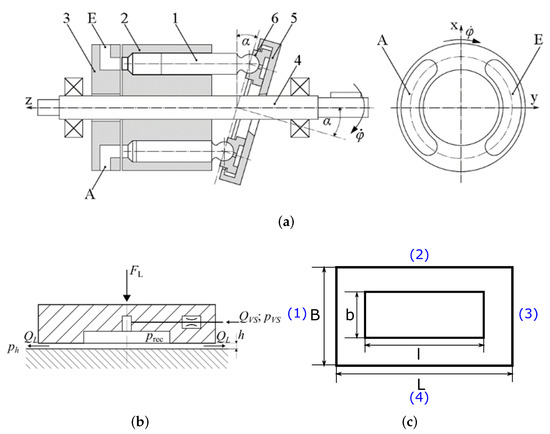
Figure 1.
Illustration of the leakage at cradle bearing in an Axial piston pump. (a) Structure of an axial piston pump in swash plate design with distributor plate [30]. 1: piston, 2: cyliner, 3: distributor plate, 4: axis, 5: swashplate, 6: sliding shoes, E: inlet, A: outlet, : Swashplate displacement : rotation velocity. (b) Pressure distribution at cradle bearing with hydrostatic lubrication. (c) A example of cradle bearing leakage model at swashplate.
The features of the regression model in this study were chosen based on an understanding of the leakage model. The tribological contact between the swashplate and cradle bearing is considered as a rectangular gap [30] and mathematically described as Equation (1), where represents the pressure difference between the pumping house and recess pressure, and stand for the width and length of the gap, respectively. Furthermore, h represents the gap where the leakage flows, and describes the fluid’s dynamic viscosity.
In order to give a clearer illustration, the leakage model of the cradle bearing is shown in Figure 1c, where the length of the cradle bearing is L, and the width is B, while the length of the recess is l and the width is b. For the leakage calculation from edge (1) and (3), , while for the leakage calculation from edge (2) and (4), . The total leakage of the cradle bearing is the sum of the leakage of edges (1) to (4). This equation shows that the leakage at the bearing is related to the pressure in the recess, the bearing’s geometry, the fluid’s dynamic viscosity, and the clearance between the swashplate and the bearing. Furthermore, at a steady state, the clearance is related to the pump’s operating point and the pressure in the recess. This study’s focus is to estimate the cradle bearing leakage at different pump operating points and recess pressures, so the temperature is kept constant in the experiment. Therefore, unlike other studies on virtual flow rate sensors [15,31], e.g., the impact of temperature was not considered in this study. In addition, since only one product was investigated in this study, the impact of geometry was not considered either. Therefore, pump operating points, including rotation speed, swashplate position, pump inlet- and outlet pressure, and recess pressure on both pump inlet- and outlet sides, were selected to construct a virtual flow rate sensor for measuring cradle bearing leakage.
2.1.2. Data Generating Using Latin Hypercube Sampling
Latin Hypercube Sampling (LHS) is a K-dimensional extension of Stratified Sampling, and Latin Square Sampling [32]. It is widely used to generate random high dimensional points for statistical experimental design and is often a better alternative to Monte Carlo sampling (MCS). MCS can also generate random points, but compared to MCS, LHS can obtain data points with the same representativeness and precision by sampling fewer points. For example, Iman [33] showed that the data variance of MCS with 1000 points is the same as that of LHS with 10 points, which shows a cost saving of a factor of 100 when using LHS instead of MCS.
The main idea of LHS is stratification [32,33], where data points are equally stratified according to the number of desired points. In general, the Stratified Sampling divides the cumulative distribution function of the random one dimensional variable vertically into N non-overlapping parts [0, 1/N), [1/N, 2/N), …, and [(N-1)/N,1]. For example, in Figure 2a, five sampling points are required to be generated, then the cumulative distribution function(CDF) is divided into five equal intervals [0, 1/5), [1/5, 2/5), …, and [4/5, 1]. Afterward, one sample point will be randomly selected in each interval [33]. The Latin Square Sampling handles the two-dimensional variable and and is shown in Figure 2b. Each variable is processed with the Stratified Sampling separately. Then, the sampled value in the same stratification is combined into a pair, and one random point will be selected. Following the same procedure, LHS deals with K-dimensional variable , ,…, .
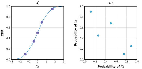
Figure 2.
A example of Stratified Sampling and Latin Square Sampling [34]. (a) Stratified Sampling. (b) The Latin Square Sampling.
In the current study, six-dimensional inputs were considered in the experiment, including pump outlet pressure, pump inlet pressure, pump speed, swashplate position, and recess pressure at the pump’s inlet side and outlet side. As described in Table 1, we consider pump outlet pressure between 10 bar and 315 bar, pump inlet pressure between 0.8 bar and 60 bar, pump speed between 1000 rpm and 3000 rpm, swashplate position between 0 % and 100 %, and recess pressure at the pump’s inlet side and outlet side varying between 0 % to 100 % and 0 % to 80 % of the pump outlet pressure. We used the maximin criterion from MATLAB to generate samples of the variable in Table 1. The minimum distance between the generated points was maximized during the iterations. After the defined iterations, a Latin hypercube sample matrix is returned.

Table 1.
Experiment of Design: the Range of searched Parameters.
For the research purpose, we generated datasets of three sizes through LHS with target dataset sizes of 1780, 555, and 330. After obtaining the datasets, the datasets with recess pressure less than 1 bar and pump outlet pressure less than inlet pressure were removed based on physical constraints. Thus, we ended up with three datasets with 1609, 501, and 300 points. We will train all three datasets equally to compare the effect of the dataset size on the model performance and select the best dataset size afterward.
2.2. Data Preprocessing
The preprocessing of model features significantly impacts the model’s performance because different features are often in different ranges [35]. For each feature to contribute equally to the model, the ranges of these features should be normalized. If there is an enormous difference between features, the features with the lower value will contribute little to the model. Furthermore, the computational efficiency of the model training is also improved after the features are normalized. In addition, the distribution of label values in this study is obviously skewed. In order to find out the effect of data label distribution on the model’s performance, a comparison between labels with transformation and without transformation (NT) was performed. Two commonly-used scaling methods were considered, i.e., log transform (LT), and square root transform (SRT).
2.2.1. Fearture Normalization
The features used for model training are normalized using Z-score [36] with Equation (2),
where x is the original training data point, u is the mean of the training data, and s is the standard deviation of the training data. The mean and standard deviation are stored in the scalar function and used later for new inputs into the regression model.
2.2.2. Label Scaling
All label data were handled with SRT and LT for the training in different experiments. Figure 3 with nine subplots shows the relative histogram of label data about cradle-bearing leakage. For the subplots in Figure 3a–i, the index 1 and 2 represent the pump outlet side and the inlet side, respectively. The subplots in each row show the results of the different label transformations, and the column represents different data sizes. It is noticed that the cradle-bearing leakage performs differently at the inlet and outlet pressure sides. The label data without transformation for all data sizes for both sides lack symmetry. However, the skewness without transformation for the pump inlet side is more pronounced. Moreover, while the SRT in subplots with index 1 transforms the data to the best symmetry, the LT in subplots with index 2 shows the best transformation result. As a result, except utilizing SRT and LT on the label data for both pressure sides, the SRT on the data for the outlet pressure side and the LT on the inlet pressure side were carried out additionally.
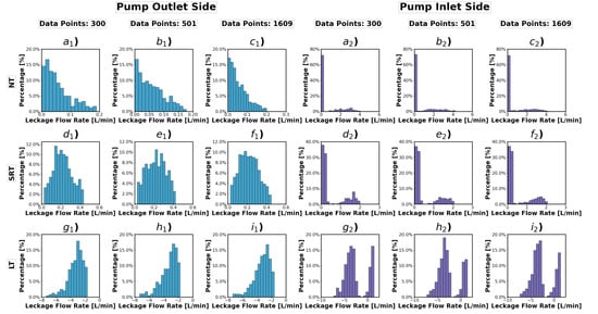
Figure 3.
Relative histogram of label data with different data sizes and label transformation method. () Model: 300 data points about leakage at pump outlet side without transformation. () Model: 501 data points about leakage at pump outlet side without transformation. () Model: 1609 data points about leakage at pump outlet side without transformation. () Model: 300 data points about leakage at pump outlet side using SRT. () Model: 501 data points about leakage at pump outlet sideusing SRT. () Model: 1609 data points about leakage at pump outlet side using SRT. () Model: 300 data points about leakage at pump outlet side using LT. () Model: 501 data points about leakage at pump outlet sideusing LT. () Model: 1609 data points about leakage at pump outlet side using LT. () Model: 300 data points about leakage at pump inlet side without transformation. () Model: 501 data points about leakage at pump inlet side without transformation. () Model: 1609 data points about leakage at pump inlet side without transformation. () Model: 300 data points about leakage at pump inlet side using SRT. () Model: 501 data points about leakage at pump inlet sideusing SRT. () Model: 1609 data points about leakage at pump inlet side using SRT. () Model: 300 data points about leakage at pump inlet side using LT. () Model: 501 data points about leakage at pump inlet side using LT. () Model: 1609 data points about leakage at pump inlet side using LT.
2.3. Regression Model Design
In this study, regression models for data-driven flow sensors are developed using the following methods: neural network (NN), support vector regression (SVR), and Gaussian regression (GR). For each training, the best hyperparameters were obtained based on the grid search performed by the score for the final evaluation. The machine learning algorithms in the sklearn library [37] were used in the program.
2.3.1. Neural Network
Neural Network has been actively used in research projects in the last decades, from supervised and unsupervised learning to reinforcement learning. Various neural networks have been developed and well studied, such as recurrent neural networks, convolutional neural networks, Long short-term memory, and feed-forward neural networks. As a three-layer neural network can arbitrarily approximate any continuous and discrete multivariate functions [38,39], it was considered in the current research. A four-layer Feed Forward Neural Network was also utilized to build a more complex function for the multi-output regression.
In Figure 4, a fully connected three-layer neural network is shown on the left. The leftmost layer is the input layer, which receives the feature signals. The value from the input layer is passed forward, multiplied with the weights of the hidden layer, and then transformed with a nonlinear activation function before being passed to the output layer. The activation function of the hidden layer in this study was chosen as the rectified linear activation function (ReLU) function, described by Equation (3). ReLU has become the default activation function for many different neural networks since models using it are easier to train and often achieve better performance.
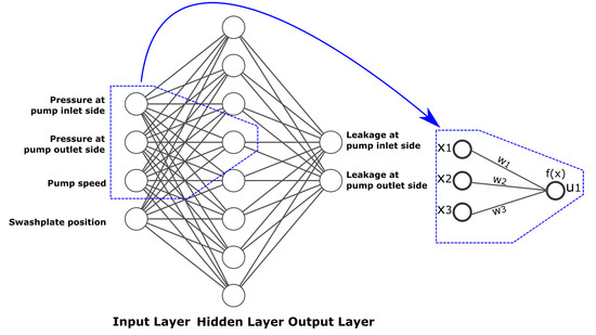
Figure 4.
A three layer feed forward neural network with description of artificial neurons.
The output layer deals with the hidden layer signal and weights but follows no activation function. The detailed illustration of artificial neurons is shown on the right side in Figure 4. In addition, the mathematical description of the neuron is shown as Equation (4), where represents the neuron output, is the neuron input, and is the weight.
During the training process, different solvers for weight optimization, learning rate , batch size , regularization term , and the size of hidden layer are studied.
2.3.2. Support Vector Regression
Support Vector learning is one of the standard machine learning methods [40,41,42]. The basic idea of SVR is to find a function , which estimates the target value according to the feature x. The SVR model guarantees an estimation error smaller than , and ignores the error if it is smaller than . At the same time the function should be as fast as possible [43]. is denoted as Equation (5)
where represents the space of the input features. The goal of the optimization is shown as Equation (6) [43]
where the slack variables are introduced to tolerate the correct margin boundary and make the optimization problem feasible, and the constant changes the trade-off between the flatness of and the tolerance . The soft margin loss setting for a linear SVM and the function of are visualized in Figure 5.
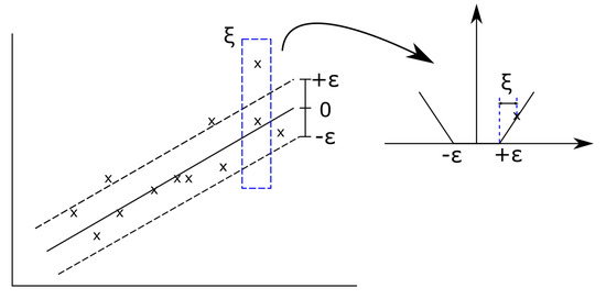
Figure 5.
The soft margin loss setting for a linear SVM [44].
In the current research, the SVR algorithm with kernel function is implemented. The dataset is transferred into another space with the kernel function, enabling a linear learning algorithm to learn a nonlinear function. The present training process with SVR includes studying kernel function , regularization parameter C, kernel coefficient , the width of error tube , and the degree of the polynomial kernel function . The details of the algorithms are well introduced in [42].
2.3.3. Gaussian Regression
To solve the Gaussian regression problem the Gaussian processes [45] are implemented. As per Equation (7), the available dataset and the new data point are assumed to fit a Gaussian distribution with mean of 0.
where K is the suitable covariance function, also called the kernel function. According to the conditional distribution property of the multidimensional Gaussian distribution,
According the properties of the Gaussian distribution is maximum when . Thus, the regression problem is solved by finding the suitable kernel function and the mean function. In the current research, to solve the Gaussian regression problem, different kernel functions, the value added to the diagonal of the kernel matrix , and the number of restarts of the optimizer for finding the kernel’s parameters n are studied.
2.4. Performance Indicator
In this study, the coefficient of determination [46] described by Equation (9) is used as a performance metric, which indicates the best estimator during the grid search for hyperparameters and shows the final testing and evaluation results of the model.
The value of varies from negative values to 1. The best value for is 1, which means the performance is better as the value gets closer to 1. If the value is negative, the performance of the model is very poor. In addition, 0 means that the prediction of the labels has no relationship with the input feature values.
2.5. Experiment Setup
Table 2 lists the 12 experimental setups. Experiments 1 to 4 applied NN and performed different transformation strategies for the label data: no transformation for both outputs, SRT for both outputs, LT for both outputs, and SRT at the pump outlet side and LT at the pump inlet side. Experiments 5 to 8 and 9 to 12 were trained for SVT and GP, respectively. The transformation for the label data was the same as for experiments 1 to 4. In addition, to select the best hyperparameters, the grid search method was utilized during each experiment. The search range of the hyperparameters is described in the rightmost column. Since this experimental setup is valid for three different datasets, there are 36 experiments in the current study.
Table 2.
Experiments of regression model training process.
3. Results
In Table 3, the results of 36 experiments using different data sizes, label scaling strategies, and regression algorithms are presented. The experimental results contain the training process score and the scores of the test data. Since the model contains two output signals, represents the average of the scores of the two outputs. The training score in this result refers to the average scores on the validation dataset during the 10-fold cross-validation. The test score represents the final evaluation of the test dataset after training. Moreover, each set of experiment results is the best outcome over the hyperparameter optimization process.
Table 3.
Model Performance.
Table 3 shows that NN has the highest test scores of 0.97, 0.95, and 0.99 for each dataset, and all scores are above 0.88 for all datasets and labeling strategies. In addition, NN delivers nearly perfect model performance in the maximal dataset, scoring above 0.98 for all label scaling strategies. In contrast, both SVR and GP exhibit high sensitivity to label scaling methods. Their scores drift as high as 0.4 on the maximal dataset. The LT + LT or SRT + LT transformations strongly impact the model performance, making the model the worst performer in each dataset. For example, the GP model for the maximal dataset drops from 0.95 to 0.55 after implementing the LT + LT label scaling method, and SVR drops from 0.90 to 0.54 after implementing the SRT + LT label scaling method. Moreover, the score of the experiment with label scaling decreases compared to the score without label scaling. Furthermore, although these drops were present in both training and test scores, the drop in test scores was more pronounced than in training scores.
To visualize the impact of different factors on model performance with the information provided by Table 3, Figure 6 is illustrated. The location of the dots indicates the utilized regression model and the method of label data processing, where the x-axis provides the method of label processing, and the y-axis provides information on the regression model. The color of the dots indicates the level of the test score, with closer to purple indicating a higher score and closer to yellow indicating a lower score. The three subplots in Figure 6a–c show the experimental results for data sizes 300, 501 and 1609. It can be seen from the plots that NN has the best model performance because dark circles in all datasets and with different label scaling methods represent the results consistently. In contrast, SVR and GR show relatively lighter colors when applying LT + LT or SRT + LT label scaling.
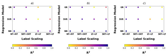
Figure 6.
Visualization of to Model and label. (a) Model: 300 data points. (b) Model: 501 data points. (c) Model: 1609 data points.
In addition, we demonstrate the performance of the NN, SVR, and GP on the test dataset in Figure 7, Figure 8 and Figure 9, respectively. There are 24 subplots in each figure, and the x-axis of each subplot represents the predicted values of the test data, while the y-axis represents the labeled values of the test data. The solid blue line is the function y = x, which indicates the ideal situation where the predicted values match the labeled values, while the “*” indicates the test results. For the 24 subplots a–l, the indexes 1 and 2 represent the pump outlet side and the inlet side, respectively. In addition, the plots in each row show the results of the different labeling of the dataset. Moreover, the column indicates the different data sizes utilized for each subplot.
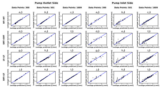
Figure 7.
Neural Network Test Results Visualization. () Model: 300 data points without transformation on both sides of the pump. () Model: 501 data points without transformation on both sides of the pump. () Model: 1609 data points without transformation on both sides of the pump. () Model: 300 data points using SRT on both sides of the pump. () Model: 501 data point susing SRT on both sides of the pump. () Model: 1609 data points using SRT on both sides of the pump. () Model: 300 data points using LT on both sides of the pump. () Model: 501 data point susing LT on both sides of the pump. () Model: 1609 data points using LT on both sides of the pump. () Model: 300 data points using SRT on data of pump’s outlet side and LT on data of pump’s inlet side. () Model: 501 data points using SRT on data of pump’s outlet side and LT on data of pump’s inlet side. () Model: 1609 data points using SRT on data of pump’s outlet side and LT on data of pump’s inlet side.
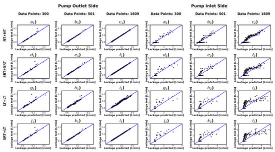
Figure 8.
Support Vector Regression Test Results Visualization. () Model: 300 data points without transformation on both sides of the pump. () Model: 501 data points without transformation on both sides of the pump. () Model: 1609 data points without transformation on both sides of the pump. () Model: 300 data points using SRT on both sides of the pump. () Model: 501 data point susing SRT on both sides of the pump. () Model: 1609 data points using SRT on both sides of the pump. () Model: 300 data points using LT on both sides of the pump. () Model: 501 data point susing LT on both sides of the pump. () Model: 1609 data points using LT on both sides of the pump. () Model: 300 data points using SRT on data of pump’s outlet side and LT on data of pump’s inlet side. () Model: 501 data points using SRT on data of pump’s outlet side and LT on data of pump’s inlet side. () Model: 1609 data points using SRT on data of pump’s outlet side and LT on data of pump’s inlet side.
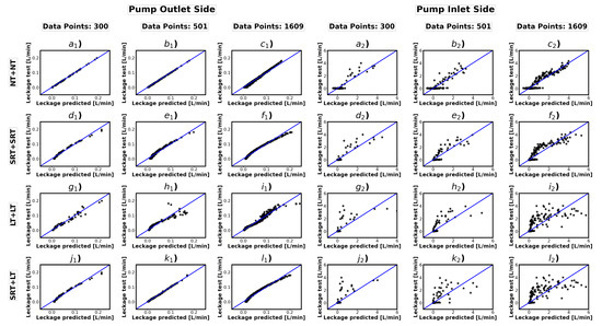
Figure 9.
Gaussian Process Regression Test Results Visualization. () Model: 300 data points without transformation on both sides of the pump. () Model: 501 data points without transformation on both sides of the pump. () Model: 1609 data points without transformation on both sides of the pump. () Model: 300 data points using SRT on both sides of the pump. () Model: 501 data point susing SRT on both sides of the pump. () Model: 1609 data points using SRT on both sides of the pump. () Model: 300 data points using LT on both sides of the pump. () Model: 501 data point susing LT on both sides of the pump. () Model: 1609 data points using LT on both sides of the pump. () Model: 300 data points using SRT on data of pump’s outlet side and LT on data of pump’s inlet side. () Model: 501 data points using SRT on data of pump’s outlet side and LT on data of pump’s inlet side. () Model: 1609 data points using SRT on data of pump’s outlet side and LT on data of pump’s inlet side.
From the three graphs in a row, we can better observe the effect of data size on model performance. The point * is closer to the ideal blue line with more data. For 1609 data points, the predicted and labeled values of NN and SVR overlap very well. Furthermore, we can observe that the method of label scaling affects the model’s performance strongly. For the NN and SVR, the impact is more evident at the pump inlet side, while for the GP it is well noticed in all cases. In addition, the model performs better for the pump outlet side, where the prediction points better agree with the ideal matter. In contrast, the prediction points show more significant variance and error for the pump inlet side.
4. Discussion
On the one hand, the current study aims to broaden the application area of data-driven flow sensors and, on the other hand, to complete the research gap on the influence of label distribution and data volume on the development of data-driven flow sensors. For the research purposes above, the following three research questions were answered:
- 1.
- Does the data-driven flow rate sensor model in the current research achieve the equivalent or better performance than the earlier study about the data-driven flow rate sensor?
- 2.
- How does the label distribution affect the performance of the data-driven flow rate sensor?
- 3.
- How does the data amount influence the performance of the data-driven flow rate sensor?
Three different regression algorithms were examined with hyperparameter optimization. The results show that the multi-output data-driven flow rate sensor performs satisfactorily in observing cradle-bearing leakage in axial piston pumps. The best model trained with the NN algorithm achieves an of 0.99, which means that the predicted values match the labeled values very well and beat the performance shown in the earlier studies [15,47]. This result proves the feasibility of a data-driven flow rate sensor in a new application area. In addition, the study results show that the distribution of labels has a strong influence on the model performance when using the GP and SVR algorithms. In contrast, the performance of the NN algorithm is independent of the label distribution. The study also shows a correlation between data volume and model performance, with data size having the most significant impact on model performance for the SVR and NN algorithms.
By answering the research questions, this study provides the following academic contributions as well as implications:
- 1.
- It extends the application area of data-driven flow sensors and is an optimized guideline for developing virtual sensors in methodology.
- 2.
- The impact of data size on the accuracy of developing data-driven flow sensors is systematically investigated. Three different data groups guarantee the model’s accuracy when labeled data are not transformed. Therefore small data can meet the model’s needs when predicting flow rate with a data-driven approach. The application areas of data-driven flow sensors are diverse, and AI models’ performance and data requirements vary significantly from application to application. Consequently, this research cannot provide general guidance for different applications, but the implications of the results of this study play a significant role in guiding us on how to design real-world data generation experiments effectively. In industrial applications, where lack of data volume or expensive data acquisition process is common, it is essential to analyze the problem with simulated data for scenarios before real-world data collection.
- 3.
- We propose an additional data preprocessing step for developing data-driven flow sensors to handle the skewed distribution of labeled data. The results suggest that, especially when using SVR or GP as a training model, the distribution of the labeled data should be analyzed and processed before training the model to obtain better performance.
The methodology and findings gained from the current research are meaningful. However, the direct transaction of the virtual sensor to the actual product may be limited by the data inaccuracy of the simulation. Further research is needed to verify the accuracy of the predictions using experimental data from the test rig. Since the data generation process is very time-consuming and expensive, we will refer to the results with simulated data to effectively collect data for the investigated axial piston pump.
Author Contributions
Conceptualization, M.L.; methodology, M.L. and G.K.; software, M.L. and G.K.; validation, M.L.; writing—original draft preparation, M.L. and G.K.; writing—review and editing, M.L., K.B. and M.G.; visualization, M.L. and G.K.; supervision, M.G. and K.B.; project administration, K.B. All authors have read and agreed to the published version of the manuscript.
Funding
This research received no funding.
Institutional Review Board Statement
Not applicable.
Informed Consent Statement
Not applicable.
Data Availability Statement
Not applicable.
Conflicts of Interest
The authors declare no conflict of interest.
References
- Geimer, M. Mobile Working Machines; SAE International: Warrendale, PA, USA, 2020. [Google Scholar] [CrossRef]
- Gärtner, M. Verlustanalyse am Kolben-Buchse-Kontakt von Axialkolbenpumpen in Schrägscheibenbauweise. Ph.D. Thesis, RWTH Aachen University, Düren, Germany, 2020. [Google Scholar]
- Mohn, G.; Nafz, T. Swash Plate Pumps—The Key to the Future. In Proceedings of the 10th International Fluid Power Conference (10. IFK), Dresden, Germany, 8–10 March 2016; Technical University Dresden: Dresden, Germany, 2016; pp. 139–149. [Google Scholar]
- Xu, B.; Hu, M.; Zhang, J.H.; Mao, Z.B. Distribution Characteristics and Impact on Pump’s Efficiency of Hydro-mechanical Losses of Axial Piston Pump over Wide Operating Ranges. J. Cent. South Univ. 2017, 24, 609–624. [Google Scholar] [CrossRef]
- Haug, S.; Geimer, M. Optimization of Axial Piston Units Based on Demand-driven Relief of Tribological Contacts. In Proceedings of the 10th International Fluid Power Conference (10. IFK), Dresden, Germany, 8–10 March 2016; Technical University Dresden: Dresden, Germany, 2016; pp. 295–306. [Google Scholar]
- Geffroy, S.; Bauer, N.; Mielke, T.; Wegner, S.; Gels, S.; Murrenhoff, H.; Schmitz, K. Optimization of the Tribological Contact of Valve Plate and Cylinder Block within Axial Piston Machines. In Proceedings of the 12th International Fluid Power Conference (12. IFK), Dresden, Germany, 9–11 March 2020; Technical University Dresden: Dresden, Germany, 2020; pp. 389–398. [Google Scholar]
- Geffroy, S.; Wegner, S.; Gels, S.; Schmitz, K. Experimental Investigation of New Design Concepts for the Tribological Contact between the Valve Plate and the Cylinder Block in Axial Piston Machines. In Proceedings of the 17th Scandinavian International Conference on Fluid Power, Linkoping, Sweden, 1–2 June 2021; pp. 104–116. [Google Scholar] [CrossRef]
- Liu, M.; Geimer, M. Estimation and Evaluation of Energy Optimization Potential with Machine Learning Method for Active Hydrostatic Lubrication Control at Cradle Bearing in Axial Piston Pump. In Proceedings of the 13th International Fluid Power Conference (IFK), Aachen, Germany, 13–15 June 2022; RWTH Aachen University: Aachen, Germany, 2022; pp. 539–550. [Google Scholar]
- Manring, N.D. The Discharge Flow Ripple of an Axial-Piston Swash-Plate Type Hydrostatic Pump. J. Dyn. Syst. Meas. Control. 1998, 122, 263–268. [Google Scholar] [CrossRef]
- Ivantysynova, M.; Huang, C. Investigation of the flow in displacement machines considering elastohydrodynamic effect. In Proceedings of the the Fifth JFPS International Symposium on Fluid Power, Nara, Japan, 12–15 November 2002; Volume 1, pp. 219–229. [Google Scholar]
- Li, F.; Wang, D.; Lv, Q.; Haidak, G.; Zheng, S. Prediction on the lubrication and leakage performance of the piston–cylinder interface for axial piston pumps. Proc. Inst. Mech. Eng. Part C J. Mech. Eng. Sci. 2019, 233, 5887–5896. [Google Scholar] [CrossRef]
- Bergada, J.; Kumar, S.; Davies, D.; Watton, J. A complete analysis of axial piston pump leakage and output flow ripples. Appl. Math. Model. 2012, 36, 1731–1751. [Google Scholar] [CrossRef]
- Özmen, Ö.; Sinanoğlu, C.; Caliskan, A.; Badem, H. Prediction of leakage from an axial piston pump slipper with circular dimples using deep neural networks. Chin. J. Mech. Eng. 2020, 33, 28. [Google Scholar] [CrossRef]
- Bikmukhametov, T.; Jäschke, J. First Principles and Machine Learning Virtual Flow Metering: A Literature Review. J. Pet. Sci. Eng. 2020, 184, 106487. [Google Scholar] [CrossRef]
- Al-Qutami, T.A.; Ibrahim, R.; Ismail, I.; Ishak, M.A. Development of Soft Sensor to Estimate Multiphase Flow Rates Using Neural Networks and Early Stopping. Int. J. Smart Sens. Intell. Syst. 2017, 10, 199–222. [Google Scholar] [CrossRef]
- Al-Qutami, T.A.; Ibrahim, R.; Ismail, I. Hybrid Neural Network and Regression Tree Ensemble Pruned by Simulated Annealing for Virtual Flow Metering Application. In Proceedings of the 2017 IEEE International Conference on Signal and Image Processing Applications (ICSIPA), Kuching, Malaysia, 12–14 September 2017; pp. 304–309. [Google Scholar] [CrossRef]
- Shoeibi Omrani, P.; Dobrovolschi, I.; Belfroid, S.; Kronberger, P.; Munoz, E. Improving the Accuracy of Virtual Flow Metering and Back-Allocation through Machine Learning. In Proceedings of the Abu Dhabi International Petroleum Exhibition and Conference, Abu Dhabi, United Arab Emirates, 12–15 November 2018. [Google Scholar] [CrossRef]
- Fortuna, L.; Graziani, S.; Rizzo, A.; Xibilia, M.G. Soft Sensors for Monitoring and Control of Industrial Processes; Springer: London, UK, 2007; Volume 22. [Google Scholar]
- Ahmadi, M.A.; Ebadi, M.; Shokrollahi, A.; Majidi, S.M.J. Evolving Artificial Neural Network and Imperialist Competitive Algorithm for Prediction Oil Flow Rate of the Reservoir. Appl. Soft Comput. 2013, 13, 1085–1098. [Google Scholar] [CrossRef]
- Patil, P.; Sharma, S.C.; Paliwal, V.; Kumar, A. ANN Modelling of Cu Type Pmega Vibration Based Mass Flow Sensor. Procedia Technol. 2014, 14, 260–265. [Google Scholar] [CrossRef][Green Version]
- Patil, P.P.; Sharma, S.C.; Jain, S. Prediction Modeling of Coriolis Type Mass Flow: Sensor Using Neural Network. Instruments Exp. Tech. 2011, 54, 435–439. [Google Scholar] [CrossRef]
- Ghanbarzadeh, S.; Hanafizadeh, P.; Saidi, M.H.; Boozarjomehry, R.B. Intelligent Regime Recognition in Upward Vertical Gas-Liquid Two Phase Flow Using Neural Network Techniques. In Proceedings of the ASME 2010 3rd Joint US-European Fluids Engineering Summer Meeting: Volume 2, Fora, Fluids Engineering Division Summer Meeting, Montreal, QC, Canada, 1–5 August 2010; pp. 293–302. [Google Scholar] [CrossRef]
- AL-Qutami, T.A.; Ibrahim, R.; Ismail, I.; Ishak, M.A. Radial Basis Function Network to Predict Gas Flow Rate in Multiphase Flow. In Proceedings of the the 9th International Conference on Machine Learning and Computing, Singapore, 24–26 February 2017; Association for Computing Machinery: New York, NY, USA, 2017; pp. 141–146. [Google Scholar] [CrossRef]
- Loh, K.; Omrani, P.S.; van der Linden, R. Deep Learning and Data Assimilation for Real-Time Production Prediction in Natural Gas Wells. arXiv 2018, arXiv:1802.05141. [Google Scholar]
- Andrianov, N. A Machine Learning Approach for Virtual Flow Metering and Forecasting. IFAC-PapersOnLine 2018, 51, 191–196. [Google Scholar] [CrossRef]
- AL-Qutami, T.A.; Ibrahim, R.; Ismail, I.; Ishak, M.A. Virtual Multiphase Flow Metering Using Diverse Neural Network Ensemble and Adaptive Simulated Annealing. Exp. Syst. Appl. 2018, 93, 72–85. [Google Scholar] [CrossRef]
- Zheng, G.B.; Jin, N.D.; Jia, X.H.; Lv, P.J.; Liu, X.B. Gas–Liquid Two Phase Flow Measurement Method Based on Combination Instrument of Turbine Flowmeter and Conductance Sensor. Int. J. Multiph. Flow 2008, 34, 1031–1047. [Google Scholar] [CrossRef]
- Wang, L.; Liu, J.; Yan, Y.; Wang, X.; Wang, T. Gas-Liquid Two-Phase Flow Measurement Using Coriolis Flowmeters Incorporating Artificial Neural Network, Support Vector Machine, and Genetic Programming Algorithms. IEEE Trans. Instrum. Meas. 2017, 66, 852–868. [Google Scholar] [CrossRef]
- Chati, Y.S.; Balakrishnan, H. A Gaussian Process Regression Approach to Model Aircraft Engine Fuel Flow Rate. In Proceedings of the 2017 ACM/IEEE 8th International Conference on Cyber-Physical Systems (ICCPS), Pittsburgh, PA, USA, 18–21 April 2017; pp. 131–140. [Google Scholar]
- Ivantysyn, J.; Ivantysynova, M. Hydrostatic Pumps and Motors: Principles, Design, Performance, Modelling, Analysis, Control and Testing, 1st ed.; Akad. Books Internat: New Delhi, India, 2001. [Google Scholar]
- Saad, Z.; Osman, M.K.; Omar, S.; Mashor, M. Modeling and Forecasting of Injected Fuel Flow Using Neural Network. In Proceedings of the 2011 IEEE 7th International Colloquium on Signal Processing and its Applications, Penang, Malaysia, 4–6 March 2011; pp. 243–247. [Google Scholar] [CrossRef]
- Mckay, M.D.; Beckman, R.J.; Conover, W.J. A Comparison of Three Methods for Selecting Values of Input Variables in the Analysis of Output From a Computer Code. Technometrics 2000, 42, 55–61. [Google Scholar] [CrossRef]
- Iman, R.L. Latin Hypercube Sampling. In Encyclopedia of Quantitative Risk Analysis and Assessment; Melnick, E.L., Everitt, B.S., Eds.; John Wiley & Sons, Ltd.: Chichester, UK, 2008. [Google Scholar] [CrossRef]
- Li, X. Numerical Methods for Engineering Design and Optimization; Lecture Notes; CRC Press: Boca Raton, FL, USA, 2014. [Google Scholar]
- Kotsiantis, S.B.; Kanellopoulos, D.; Pintelas, P.E. Data preprocessing for supervised leaning. Int. J. Comput. Sci. 2006, 1, 111–117. [Google Scholar]
- Brase, C.H.; Brase, C.P. Understanding Basic Statistics, 4th ed.; Houghton Mifflin: Boston, MA, USA, 2007. [Google Scholar]
- Pedregosa, F.; Varoquaux, G.; Gramfort, A.; Michel, V.; Thirion, B.; Grisel, O.; Blondel, M.; Prettenhofer, P.; Weiss, R.; Dubourg, V.; et al. Scikit-learn: Machine Learning in Python. J. Mach. Learn. Res. 2011, 12, 2825–2830. [Google Scholar]
- Hecht-Nielsen, R. Kolmogorov’s Mapping Neural Network Existence Theorem. In Proceedings of the the International Conference on Neural Networks, San Diego, CA, USA, 21–24 June 1987; IEEE Press: New York, NY, USA, 1987; Volume 3, pp. 11–14. [Google Scholar]
- Ismailov, V. A three layer neural network can represent any multivariate function. arXiv 2020, arXiv:2012.03016. [Google Scholar]
- Cherkassky, V.; Mulier, F. Learning from Data: Concepts, Theory, and Methods; IEEE Press: Piscataway, NJ, USA; Wiley: Hoboken, NJ, USA, 2007. [Google Scholar]
- Hearst, M.; Dumais, S.; Osuna, E.; Platt, J.; Scholkopf, B. Support vector machines. IEEE Intell. Syst. Their Appl. 1998, 13, 18–28. [Google Scholar] [CrossRef]
- Smola, A.J.; Schölkopf, B. A tutorial on support vector regression. Stat. Comput. 2004, 14, 199–222. [Google Scholar] [CrossRef]
- Cortes, C.; Vapnik, V. Support-vector networks. Mach. Learn. 1995, 20, 273–297. [Google Scholar] [CrossRef]
- Schölkopf, B. Learning with Kernels: Support Vector Machines, Regularization, Optimization, and Beyond; Adaptive Computation and Machine Learning; MIT Press: Cambridge, MA, USA, 2002. [Google Scholar] [CrossRef]
- Rasmussen, C.E.; Williams, C.K.I. Gaussian Processes for Machine Learning, 3rd ed.; Adaptive Computation and Machine Learning; MIT Press: Cambridge, MA, USA, 2008. [Google Scholar]
- Lewis-Beck, C.; Lewis-Beck, M.S. Applied Regression: An Introduction, 2nd ed.; Sage University Papers, Quantitative Applications in the Social Sciences; Sage: Thousand Oaks, CA, USA; London, UK; New Delhi, India, 2016; Volume 22. [Google Scholar]
- Berneti, S.M.; Shahbazian, M. An imperialist competitive algorithm artificial neural network method to predict oil flow rate of the wells. Int. J. Comput. Appl. 2011, 26, 47–50. [Google Scholar]
Publisher’s Note: MDPI stays neutral with regard to jurisdictional claims in published maps and institutional affiliations. |
© 2022 by the authors. Licensee MDPI, Basel, Switzerland. This article is an open access article distributed under the terms and conditions of the Creative Commons Attribution (CC BY) license (https://creativecommons.org/licenses/by/4.0/).