Article

Microgrid Harmonic Mitigation Strategy Based on the Optimal Allocation of Active Power and Harmonic Mitigation Capacities of Multi-Functional Grid-Connected Inverters

Key Lab of Power Electronics for Energy Conservation and Motor Drive of Hebei Province, Yanshan University, Qinhuangdao 066004, China
*
Author to whom correspondence should be addressed.
Energies 2022, 15(17), 6109; https://doi.org/10.3390/en15176109
Submission received: 29 July 2022 / Revised: 21 August 2022 / Accepted: 22 August 2022 / Published: 23 August 2022
(This article belongs to the Topic Power Quality)

Abstract

:
Harmonic pollution sources in microgrids have the characteristics of high penetration and decentralization, as well as forming a full network. Local harmonic mitigation is a traditional harmonic mitigation method, which has the disadvantages of complexity and costly operation. Based on the idea of the decentralized autonomy of power quality, this paper establishes a comprehensive optimization model of the active power and harmonic mitigation capacities of grid-connected inverters based on two-layer optimization and realizes harmonic mitigation. Firstly, based on the harmonic sensitivity analysis, the calculation method of harmonic mitigation capacity is given. Secondly, a two-layer model of harmonic mitigation optimization is established. The upper-layer optimization model takes the minimum operation cost of the microgrid as the objective and the active power reduction in the multi-functional grid-connected inverter (MFGCI) as the optimization variable. The lower-layer optimization model offers the best harmonic mitigation effect as the objective and the harmonic current compensation as the optimization variable. According to the relationship between the total remaining capacity of MFGCI and the capacity required for harmonic mitigation, there are three different objective functions in the lower-layer optimization model. Then, the model solving steps are provided. Finally, an example shows that the proposed optimization model can achieve harmonic mitigation at different times. Compared with the case without active power optimization, the operation cost of the whole system can be reduced by up to 14.6%, while ensuring the harmonic mitigation effect. The proposed method has the advantages of a harmonic mitigation effect and economical system operation.

1. Introduction

With the development and use of a large number of new energy devices, the random and massive access of non-linear loads, and the normalization of network power electronics, the harmonic pollution of microgrids is becoming a pressing issue [1,2]. On the one hand, with continuous expansion in the size of the microgrid, the distribution range of and level of pollution from harmonic sources are gradually increasing. The ability of microgrids to absorb power quality pollution is weak, and the powerful electronic equipment in the network is susceptible to power quality and has high requirements for waveforms, amplitude and frequency. This makes the power quality problem of microgrids even more pressing [3,4]. In [5], a medium-sized industrial microgrid is calculated shows that the levels of total harmonic distortion have exceeded the limit value imposed in the standard. On the other hand, due to the decentralized and wide-area characteristics of microgrid harmonic sources [6], the traditional method of centralized mitigation has the problems of a high installation cost of equipment, single function, and low utilization of equipment capacity, making it more difficult to meet the increasingly complex mitigation needs of network distribution and unsuitable for new energy microgrids with a decentralized distribution of multiple harmonic sources. Therefore, there is an urgent need to seek a power-quality mitigation method for local mitigation of harmonic pollution sources.
It is demonstrated that a multi-functional grid-connected inverter (MFGCI) can mitigate power-quality pollution on a local scale. The MFGCI has the same topology as the active power filter (APF) and only requires appropriate software upgrades to enable the integration of renewable energy, while considering the improvement of microgrid power quality [7]. With its multitasking function, MFGCI not only improves the cost performance of grid-connected inverters, but also reduces investment costs by avoiding the installation of additional power-quality improvement devices in the microgrid.
In previous research on MFGCI structures, a sliding mode controller and a positive fundamental component estimator were used to calculate current and voltage to realize the simultaneous outputs of the active power and reactive power of MFGCI [8]. In [9], the design, development and implementation process of the MFGCI laboratory prototype with APF function is described. In [10], a new type of MFGCI was studied. The MFGCI is composed of a three-phase DC/AC converter with three ports and a DC/DC converter at the front stage, and a 5kVA laboratory prototype was designed, which cannot only output active power but also compensate for harmonic current and reactive power. In [11], MFGCI is proposed with the function of compensating harmonic current, reactive power and the three-phase imbalance on the basis of considering the power quality of microgrids and the effectiveness of grid-connected inverters.
To more effectively control reactive power and voltage, a type of shutdown series-switched MFGCI (SSS-MFGCI) was proposed in [12], which achieved the four-quadrant operation of SSS-MFGCI through a bidirectional switch commutation method. In [13], a MFGCI control scheme was designed that can suppress both steady and dynamic disturbances; the control scheme includes an inner-loop controller and an improved reference for the current generation algorithm. From the references [8,9,10,11,12,13], we can draw a clear conclusion that MFGCI achieves harmonic compensation or harmonic mitigation.
In research on operation control strategy, the authors of [14] used SSS-MFGCI, which was first proposed in [12], and set different operation modes according to various grid disturbances to realize the control of voltage swell, voltage sag and voltage imbalance. In [15], SSS-MFGCI was applied to V2G based on [14]. In [16], an improved MFGCI power governance compensation algorithm based on the conservative power theory was proposed, and the small signal stability of MFGCI was analyzed using the impedance modeling method. In [17], MFGCI is modelled based on impedance reconstruction model, realizes the purpose of MFGCI providing virtual inertia and eliminating harmonic resonance. In [18], a multi-objective control strategy was designed, which enables the MFGCI to simultaneously output harmonic compensation current and reactive power through closed-loop active power control technology, compensating the harmonic and reactive power of the system. In [19], a virtual impedance droop control and secondary power balance control were combined, and a comprehensive control strategy for MFGCIs was proposed, which can achieve harmonic mitigation and a three-phase unbalance suppression of the grid. In [20], MFGCI can operate in shunt-connected and cascade-connected modes; therefore, the required compensation can be provided for current- or voltage-related power-quality issues with the assistance of bidirectional switches. In [21], a power management algorithm was developed to determine the optimal operating mode of the MFGCI and realize selective power injection and power regulation. From the references [14,15,16,17,18,19,20,21], it is observed that active output, reactive output and harmonic compensation can be simultaneously realized through the control algorithm of MFGCI.
However, power quality management is only an auxiliary function of MFGCI. The compensation capacity that can be used in a single MFGCI is always limited. Microgrids often contain multiple grid-connected inverters, which can play a greater role if the compensation capacity of these grid-connected inverters is aggregated. In [22], the study proposed a control method to coordinate multiple MFGCIs to participate in microgrid power quality management based on the Fryze–Buchholz–Dpenbrock (FBD) power theory. In [23], a comprehensive power-quality evaluation (CPQE) index was proposed based on the mutation theory, and a multi-objective optimal compensation model with multiple MFGCIs was established with the objectives of optimizing the CPQE index and minimizing the occupied capacity of MFGCIs used for power-quality compensation.
Similar to [23], a new comprehensive power-quality evaluation method was proposed in [24], which used the G1 method and hybrid variable weight principle to establish a multi-objective optimal compensation model containing multiple MFGCIs with the objectives of optimizing the CPQE index and minimizing the occupied capacity of MFGCIs for power-quality compensation. In addition to local management, MFGCI can also be used for targeted power-quality management of specific nodes at remote ends. In [25], a distribution control strategy of the MFGCI output current was proposed based on the remaining capacity of MFGCIs, the harmonic currents of the shunt nodes, and reactive currents of the shunt nodes. In [26], an optimization model to realize the best operation state of the MFGCI and OLTC was proposed, which offers the best results in terms of voltage quality, minimum power losses and the longest OLTC life as the optimization objectives. In [27], a new strategy for the cooperative and optimal allocation of VDAPF and SVG considering the contribution of MFGCI is proposed, focusing mainly on the capacity allocation of VDAPF and SVG. References [22,23,24,25,26,27] introduce corresponding control strategies for different application requirements, which can realize local and decentralized harmonics mitigation in microgrids. However, it cannot be ignored that the part of capacity of MFGCI needs to be occupied when compensating harmonics. Therefore, the relationship between the remaining capacity of MFGCI and the capacity required for harmonic compensation needs to be considered, and when the remaining capacity is small, some of the active power capacity can be appropriately reduced to improve the harmonic compensation capacity. A photovoltaic (PV) is connected to the grid through MFGCI.
In research on PV active power control, a new type of photovoltaic power generation module and its control strategy are proposed in [28], which can ensure the continuous output of active power when the solar radiation intensity changes unexpectedly. In [29], according to the solar irradiance and cloud cover at different stages of the day, the reference value of power per hour is optimized based on random dynamic programming to realize the PV active power control. However, the reduction in active power grid-connected capacity affects the economy of microgrid operation. The allocation of the MFGCI harmonic compensation capacity and active power grid-connected capacity to ensure the economy of microgrid operations with optimal power-quality improvement has not been thoroughly studied in the references [18,19,20,21,22,23,24,25,26,27,28,29].
In order to integrate the active power grid-connected and harmonic mitigation functions of MFGCI and achieve the integrated optimization of system operation and harmonic mitigation, this paper solves the problem of allocating the active power grid-connected capacity and harmonic mitigation capacity of MFGCI through the use of microgrid active optimization and nodal harmonic mitigation. A two-layer optimization model was established for the integrated active power-harmonic mitigation capacity allocation of MFGCI, with the upper layer of active power optimization used to determine the optimal amount of MFGCIs to be connected to the grid. The lower layer for harmonic mitigation optimization determines the corresponding objective function according to the relationship between the total remaining capacity of the system and the size of the capacity required for harmonic mitigation, optimizing the harmonic mitigation scheme and the harmonic mitigation capacity of each MFGCI. A discrete binary-coded two-layer simulated annealing particle swarm algorithm (SAPSO) with a nested harmonic power flow calculation is used to solve the problem. The validation results show that the two-layer optimization model established in this paper not only ensures the optimal PV active grid-connected inverters, but also enables the harmonic mitigation of the system to achieve the best results.

2. Allocation of MFGCI Capacity

2.1. Relationship between Active Power and Remaining Capacity of MFGCI

Due to the uncertainty of renewable energy power generation, the rated capacity of grid-connected inverters is often larger than the actual power generated by wind turbines or PV panels. Moreover, due to natural factors, PV does not always operate at full power; there is always a certain remaining capacity of MFGCI. This remaining capacity can be used to realize the harmonic mitigation function. The utilization rate of the equipment can be improved by formulating a reasonable allocation strategy of MFGCI active grid-connected capacity and remaining capacity.
DG can generate active power and reactive power, assuming that the total capacity of the inverter is available. Since its rated capacity is a certain value, according to the active power output value and reactive power output value of DG at a certain time, the remaining capacity of each inverter available for harmonic mitigation at the corresponding time can be obtained, and the formula for calculating the remaining capacity S m _ remain is shown in the following equation:
S m _ remain = S m _ MFGCI 2 P m _ MFGCI 2 Q m _ MFGCI 2
where S m _ MFGCI is the rated capacity of the m-th inverter; P m _ MFGCI and Q m _ MFGCI are the active power and reactive power output of the m-th inverter, respectively.

2.2. Relationship between Compensation Current and Harmonic Compensation Capacity

The remaining capacity of MFGCI after active power connection is used to compensate for the harmonics, and the relationship between the compensation capacity required for harmonic mitigation and each emitted harmonic compensation current is:
S i _ recoup 2 = ( U i 1 2 + h = 2 H U i h 2 ) ( h = 2 H I i h 2 )
where S recoup i is the required capacity of MFGCI at node i to compensate for harmonics; U i 1 is the fundamental voltage at node i; U i h is the h-th harmonic voltage at node i;  I i h is the h-th harmonic current compensated at node i; and H is the maximum order of harmonics.
Considering that the amplitude of each harmonic voltage is smaller than the fundamental voltage, in the actual calculation, the value of each harmonic voltage can be ignored, and only the fundamental voltage is retained.
S i _ recoup 2 = U i 1 2 ( h = 2 H I i h 2 )

2.3. Harmonic Mitigation Sensitivity Analysis

The harmonic mitigation sensitivity W i j of MFGCI of node j to node i is:
W i j = h = 2 H α i h U i h I j h
where α i h is the weight accounted for by the h-th harmonic voltage at node I; I j h is the h-th harmonic current compensated at node j.
In this paper, the harmonic power flow calculation of the simulation example adopts the approximate harmonic power flow calculation method. U i h / I j h is equal to the h-th harmonic mutual impedance Z i j h between node i and node j, so that the above equation can be written as:
W i j = h = 2 H α i h Z i j h
Depending on the magnitude of W i j , the MFGCIs with the best and worst harmonic mitigation sensitivity at node i can be determined, respectively.
If the total harmonic distortion (THD) at node i in the system is the maximum, i.e., THD = Mi% (Mi > 4), then the magnitude of each harmonic voltage is Uh, respectively. If the W i j between node j connected with MFGCI and node i is the minimum, then the MFGCI at node j has the worst harmonic mitigation sensitivity to node i, and the capacity required for the harmonic mitigation of node i using the MFGCI at node j is maximum. The maximum mitigation capacity S demand _ max required to mitigate the THD of node i to 4% is shown below:
S demand _ max = λ i U j 1 ( h = 2 H U i h Z i j h )
where λ i is the difference coefficient, and its value is less than 1, depending on the difference between Mi and 4; U j 1 is the fundamental voltage at node j.
Similarly, if the W i k between node k connected with MFGCI and node i is maximum, then the MFGCI at node k has the best harmonic mitigation sensitivity with node i. The minimum capacity required for the harmonic mitigation of node i using the MFGCI at node k is minimum. The minimum mitigation capacity S demand _ min required to mitigate the THD of node i to 4% is shown below.
S demand _ min = λ i U k 1 ( h = 2 H U i h Z i k h )
where U k 1 is the fundamental voltage at node k; Z i k h is the h-th harmonic mutual impedance between node i and node k.

3. Two-Layer Optimization Model for the Comprehensive Allocation of MFGCI Active Power and Harmonic Mitigation Capacity

3.1. Modeling Ideas

When the generation power of DG is large, the remaining capacity available for harmonic mitigation has a relatively similar value. Using only the existing MFGCI remaining capacity, the system may have nodes with excessive harmonic content under the same harmonic pollution injection; and the extreme effort to achieve the power-quality index of harmonic voltage requires more MFGCI capacity for harmonic mitigation, which affects the maximum grid-connected power of DG and is not conducive to the maximum utilization of new energy, despite the improvement in power-quality. Considering the mutual constraint relationship between the active grid-connected capacity of MFGCI and the capacity of harmonic mitigation, this paper establishes a two-layer optimization model for the integrated active grid-connected and harmonic mitigation capacity allocation of MFGCI, starting from the allocation of the active grid-connected capacity and the remaining capacity of MFGCI. This optimization strategy is shown in Figure 1.

3.2. Upper Layer—Active Power Optimization

The upper layer takes the minimum system operation cost as the optimization objective, and the objective function includes the cost of purchasing and selling electricity, the cost of network power loss, the cost of inverter operation and maintenance, and the benefit of power-quality improvement. The benefits of power-quality improvement include the equivalent APF installation cost and equivalent APF operation and maintenance cost.

3.2.1. Objective Function

The total objective function of the upper layer is:
f up = min ( C en + C loss + C om E dev E om )
where C en is the cost of purchasing and selling electricity; C loss is the cost of network power loss; C om is the cost of MFGCI operation and maintenance; E dev is the cost of equivalent APF installation; E om is the cost of equivalent APF operation and maintenance. The calculation equation of each component is shown below.
  • Cost of Purchasing and Selling Electricity:
    C en = c b t Δ t ( P t m = 1 M P t m )
    where P t is the total power required by the microgrid load at time t; P t m is the active grid-connected of the m-th MFGCI at time t; Δ t is the length of each optimization period; M is the total number of MFGCIs; c b t is the real-time purchasing and selling electricity of the microgrid unit price, the expression of c b t at time t is as follows:
    c b t = { c u t P t m = 1 M P t m c s t P t < m = 1 M P t m
    where c u t is the price of purchasing electricity by microgrid from the grid at time t; c s t is the price of selling electricity by microgrid to the grid at time t.
  • Cost of Network Power Loss
Network power loss mainly considers line active power loss, and its calculation is expressed as follows:
C loss = c pu Δ t ( h i = 1 N j i j i U t i h ( U t i h U t j h ) 2 R i j )
where j i indicates that node j is directly connected to node i; U t i h and U t j h are the h-th harmonic voltage values of node i and node j at time t, respectively; R i j is the branch resistance value between node i and node j; N is the number of nodes; and c pu is the factor of network power loss cost.
  • Cost of MFGCI Operation and Maintenance:
    C om = C op + C ma
    C op = c 1 m = 1 M P t m + c 2 m = 1 M S t m _ recoup
    C ma = c MFGCI m = 1 M S m _ MFGCI
    where C op is the cost of operation of MFGCI; C ma is the cost of maintenance of MFGCI; c 1 is the cost factor of MFGCI active power grid-connected inverter; c 2 is the cost factor of MFGCI harmonic mitigation; S t m _ recoup is the capacity of the m-th MFGCI involved in harmonic mitigation at time t; and c MFGCI is the maintenance cost per unit capacity of MFGCI.
  • Cost of Equivalent APF Installation:
    E dev = c 3 m = 1 M S t m _ recoup
    where c 3 is the installed cost per unit capacity of APF.
  • Cost of Equivalent APF Operation and Maintenance:
    E om = ( c 4 + c 5 ) m = 1 M S t m _ recoup
    where c 4 is the cost factor of operation of the APF, and c 5 is the cost factor of maintenance of the APF.

3.2.2. Constraint Condition

The constraints for the upper-layer optimization are the power balance constraint, node voltage constraint, branch power constraint and control variable constraint. The specific expressions of each part are shown below.
  • Power Balance Constraint:
    { P i = U i j = 1 n U j ( G i j cos θ i j + B i j sin θ i j ) Q i = U i j = 1 n U j ( G i j sin θ i j B i j cos θ i j )
    where P i , Q i are the injected active power and reactive power of node i, respectively; U i , U j are the voltage amplitudes of nodes i and j, respectively; G i j , B i j are the real and imaginary parts of the node derivative matrix, respectively; and θ i j is the phase angle difference between the voltages of nodes i and j.
  • Node Voltage Constraint:
    U i _ min U i U i _ max
    where U i _ max and U i _ min are the upper and lower limits of the voltage amplitude at node i, respectively.
  • Branch Power Constraint:
    P l P l _ max ,   l Ω
    where P l is the active power transmitted by branch l; P l _ max is the maximum allowable value of active power transmitted by branch l; and Ω is the set of branches.
  • Control Variable Constraint:
    0 S m _ cut S m _ MFGCI
    where S m _ cut is the active power reduction in the m-th MFGCI.

3.3. Lower-Layer—Harmonic Mitigation Optimization

The lower layer is a microgrid harmonic mitigation optimization model. The maximum and minimum capacities required for harmonic mitigation can be calculated by harmonic mitigation sensitivity analysis. According to the size relationship between the total remaining capacity of MFGCI and the maximum and minimum capacity required for harmonic mitigation, the lower-layer optimization can be subdivided into three sub-objectives.

3.3.1. Objective Function I

When the sum of the total remaining capacity of the MFGCI and the installed capacity of the APF is greater than the maximum capacity required for harmonic mitigation, the remaining capacity of the MFGCI is sufficient to mitigate harmonics without reducing the active grid-connected capacity:
f down 1 = min ( m = 1 M S m _ recoup S demand _ max S APF + i = 1 N β i T H D i i = 1 N β i T H D i )
where β i is the importance coefficient of node i, which is related to the power of the load connected to node i and the requirements of the load on power-quality; S APF is the installed capacity of the APF; T H D i is the THD of node i after harmonic mitigation; T H D i is the THD of node i before harmonic mitigation.
The constraints include THD constraints [30] at each node and MFGCI harmonic mitigation capacity constraints:
T H D i 4 %
S m _ recoup S m _ remain
where S m _ remain is the remaining capacity of the m-th MFGCI.

3.3.2. Objective Function II

When the sum of the total remaining capacity of MFGCI and the installed capacity of APF is less than the minimum capacity required for harmonic mitigation, the remaining capacity of the MFGCI is not enough to mitigate harmonics, and it is necessary to reduce the active grid-connected capacity:
f down 2 = min ( m = 1 M S m _ cut S demand _ max m = 1 M S m _ remain S APF + i = 1 N β i T H D i i = 1 N β i T H D i )
The constraints include THD constraints and active power reduction constraints for each node:
T H D i 4 %
S m _ cut P m _ MFGCI
where P m _ MFGCI is the grid-connected capacity of the active power of the m-th MFGCI:

3.3.3. Objective Function III

When the sum of the total remaining capacity of MFGCI and the installed capacity of APF is between the minimum and maximum capacity required for harmonic mitigation, it is impossible to judge whether the remaining capacity of the MFGCI is sufficient to mitigate harmonics or whether it is necessary to reduce the grid-connected capacity of the active power of the MFGCI. In order to ensure that the remaining capacity of the MFGCI is preferentially used to mitigate harmonics, and to avoid the remaining capacity and partial reduction in the useful grid-connected capacity caused by some MFGCIs, the sign function sgn is added to the objective function. When the harmonic mitigation capacity of the MFGCI is greater than its remaining capacity, sgn = 1, which increases the value of the objective function. When the harmonic mitigation capacity of the MFGCI is less than its remaining capacity, sgn = −1, which makes the value of the objective function smaller. When the harmonic mitigation capacity of the MFGCI is equal to its remaining capacity, sgn = 0, meaning that the objective function value remains unchanged. The objective function is as follows.
f down 3 = min [ m = 1 M S m _ recoup S demand _ max S APF + m = 1 M sgn ( S m _ recoup S m _ remain ) + i = 1 N β i T H D i i = 1 N β i T H D i ]
The constraints include the THD constraint of each node and the harmonic mitigation capacity constraint of each MFGCI.
T H D i 4 %
S m _ recoup S m _ MFGCI
According to different operating conditions of the system, the selection of three objective functions for lower-layer optimization is shown in Figure 2.

4. Model Solving

The upper and lower models are interrelated; therefore, a fast optimization algorithm is needed. The discrete binary coded two-layer simulated annealing particle swarm optimization (SAPSO) with nested harmonic power flow calculation has the advantages of a simple and easy implementation, fast search speed and few parameter settings. It can find the global optimum in a short time. Therefore, the upper and lower objective functions are solved by SAPSO algorithm.
The upper-layer optimization solution parameters are set as follows: the particle population size is 200, the learning factor is 1.5, the inertia weight linearly decreases with a maximum value of 0.95 and minimum value of 0.7, and the maximum number of iterations is 300. The lower-layer optimization solution parameters are set as follows: the particle population size is 300, the learning factor is 1.5, the inertia weight linearly decreases with a maximum value of 0.95 and minimum value of 0.7, and the maximum number of iterations is 300.

4.1. Upper-Layer Particle Coding

In the upper-layer optimization, the optimization variable is the active power reduction; therefore, the upper-layer particle is the MFGCI active power reduction. It should be noted that a single particle can be a value or a group of values. If a microgrid contains M-th MFGCIs, each particle is composed of M-th MFGCI active power reductions. The upper-layer optimized particle structure is shown in Figure 3. In the figure, S m _ cut is the active power reduction in the m-th MFGCI.

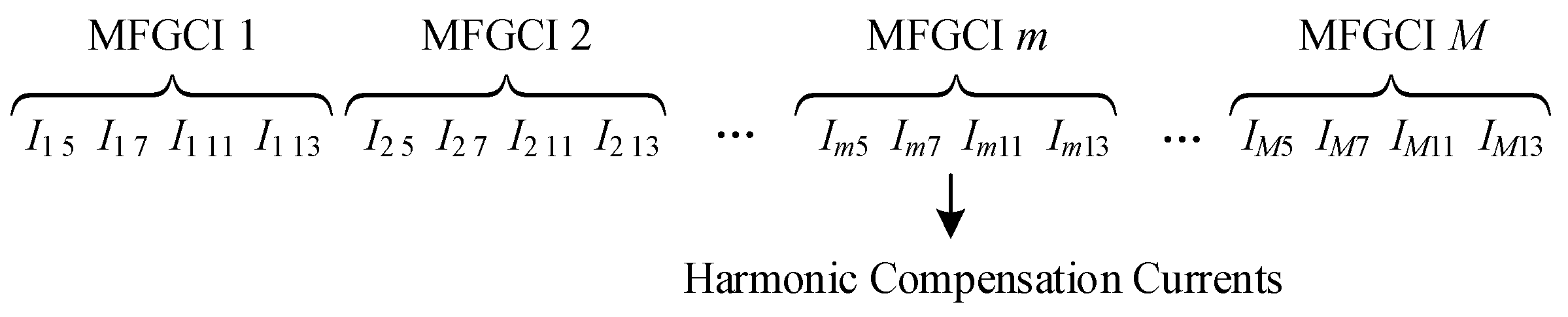
4.2. Lower-Layer Particle Coding

In the lower-layer optimization, the optimization variable is the harmonic compensation current; therefore, the lower-layer particle is the harmonic compensation current of MFGCI. In the lower-layer harmonic mitigation optimization, each particle contains an M-th harmonic compensation current of MFGCIs, and each harmonic compensation current of MFGCI is divided into 5th, 7th, 11th and 13th harmonic compensation currents. The initial state of each particle in the lower-layer optimization is randomly generated within the range determined by the upper-layer optimization results and the constraint conditions. The lower-layer particle structure is shown in Figure 4. In the figure, I m 5 , I m 7 , I m 11 , I m 13 are the 5th, 7th, 11th and 13th harmonic compensation currents output by the m-th MFGCI, respectively:

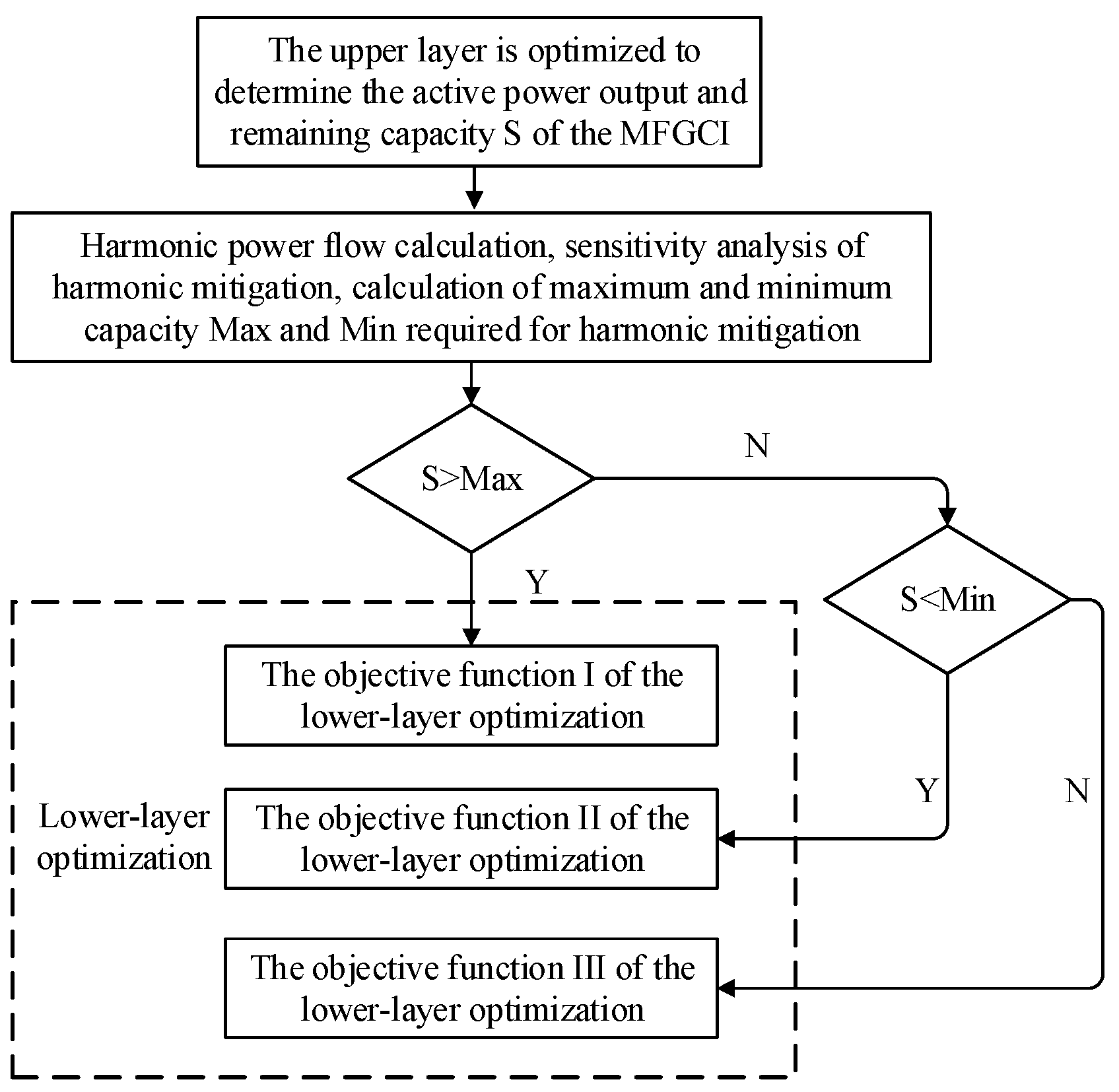
4.3. Model Solving Steps

Step 1: Collect real-time power information of photovoltaics and loads, and set the initial value of active power reduction to 0;
Step 2: Calculate the remaining capacity of the inverter that can be used for harmonic mitigation;
Step 3: Carry out harmonic power flow calculation to obtain the voltage harmonic distortion rate of each node;
Step 4: Determine whether there is a node with THD exceeding the standard in the system. If it does not exist, the optimization is over. If it exists, go to step 5;
Step 5: Perform harmonic mitigation sensitivity analysis on nodes whose THD exceeds the standard, and calculate the maximum and minimum capacity required for harmonic mitigation;
Step 6: The lower-layer optimizes particle coding and selects the corresponding objective function for harmonic mitigation optimization according to the relationship between the remaining capacity and the capacity required for harmonic mitigation;
Step 7: Determine whether the active work needs to be reduced. If not, output the optimization result, the optimization is over; if necessary, go to step 8;
Step 8: The upper layer optimizes the particle coding, performs the upper-layer active power optimization, and obtains the active power reduction in each MFGCI;
Step 9: Go to step 2 and continue to optimize until the optimal solution is obtained.
The flow chart of the model solution is shown in Figure 5.

5. Case Analysis

5.1. System Parameters

To verify the effectiveness of the model established in this paper for microgrid power-quality improvement, the IEEE 33-bus system connected to the distributed photovoltaic grid was selected as the simulation object, as shown in Figure 6. The system voltage level is 10 kV, nodes 4, 7, 22, 25 and 27 are DG grid-connected nodes, and the rated capacity of MFGCI connected to each node is shown in Table 1. Nodes 4, 9, 13, 17, 21, 24, 27 and 31 are harmonic source access nodes, and the 5th, 7th, 11th and 13th harmonics were considered. The magnitudes of the load power and harmonic sources for each harmonic current at each node at different moments are shown in the Appendix A [31]. The weight values of different harmonic voltages are shown in Table 2. Nodes 8, 20, 23 and 32 are APF access nodes, and the total installed capacity of APFs is 100 kW. Considering the low voltage level of microgrids and scattered distribution of harmonic sources, γ is 0.95. The reactive power output of MFGCI is ignored. Solar intensity data are derived from a region in the southern Hebei Province, China.
To verify the adaptability of the proposed model to different situations, the system operation was optimized with the model at three typical times: 7:00, 13:00 and 16:00, respectively.

5.2. Simulation Results

5.2.1. System Optimization Results at 7:00

According to the basic parameters of the system at 7:00, the remaining capacity of MFGCI and the maximum and minimum capacity required for harmonic mitigation can be obtained from Equations (1), (6) and (7), as shown in Table 3 and Table 4.
As observed from Table 3 and Table 4, the active power of the PV at 7:00 is small, and the remaining capacity of the MFGCI is large. The total remaining capacity is larger than the maximum capacity required for harmonic mitigation, which is sufficient to compensate for the harmonics and does not need to cut active power. Thus, objective function I is selected for the lower optimization in the process of solving the two-layer optimization model. According to the optimization results, the capacity of each MFGCI involved in harmonic mitigation can be obtained from Equation (3), and the results are shown in Table 5.
Figure 7 shows the THD of each node before and after harmonic mitigation.
The capacity of each MFGCI involved in harmonic mitigation at 7:00 is less than the remaining capacity, and the total capacity used for harmonic mitigation is 319.26 kW, which is between the maximum and minimum capacity required for harmonic mitigation. The THD of each node is less than 4% after optimization, and the capacity used for harmonic mitigation and the level of harmonic mitigation meet the requirements.

5.2.2. System Optimization Results at 13:00

According to the basic parameters of the system at 13:00, the remaining capacity of MFGCI and the maximum and minimum capacity required for harmonic mitigation can be obtained from Equations (1), (6) and (7), as shown in Table 6 and Table 7.
At 13:00, the PV active power reaches the maximum, the active power grid-connected capacity of each MFGCI also reaches the maximum, and the total remaining capacity is the minimum at this time. The sum of the total remaining capacity and the APF installed capacity is less than the minimum capacity required for harmonic mitigation, which is not enough to mitigate harmonics, so objective function II is selected for the lower-layer optimization in the process of solving the two-layer optimization model. To achieve our optimization results, the capacity of each MFGCI involved in harmonic mitigation was obtained from Equation (3), and the results are shown in Table 8.
The THD of each node before and after harmonic mitigation is shown in Figure 8.
As can be seen from Figure 8, each MFGCI at 13:00 requires active power reduction for harmonic mitigation. The total capacity required for harmonic mitigation is 375.59 kW, which lies between the maximum and minimum capacity required for harmonic mitigation. After optimization, the THD of each node is less than 4%, and the capacity used for harmonic mitigation and the level of harmonic mitigation meet the requirements.

5.2.3. System Optimization Results at 16:00

Similarly, based on the basic parameters of the system at 16:00, the remaining capacity of the MFGCI and the maximum and minimum capacities required for harmonic mitigation can be obtained, and the results are shown in Table 9 and Table 10.
At 16:00, PV is not in a full-generation state, MFGCI has some remaining capacity, the total remaining capacity is between the maximum and minimum capacity needed for harmonic mitigation. Therefore, MFGCI may or may not need to cut active power; thus, in the process of solving the two-layer optimization model, the objective function III is selected for the lower-layer optimization. According to the optimization results, the capacity of each MFGCI involved in harmonic mitigation is obtained from Equation (3), and the results are shown in Table 11.
The THD of each node before and after harmonic mitigation is shown in Figure 9.
From the above results, at 16:00, it can be observed that the MFGCIs connected at nodes 4, 25 and 27 require active power reduction, while the MFGCIs connected at nodes 7 and 22 do not, and their remaining capacities are all used for harmonic mitigation. The total capacity used for harmonic mitigation is 421.64 kW, which is between the maximum and minimum capacity required for harmonic mitigation. After optimization, the THD of each node is less than 4%, and the capacity used for harmonic mitigation and its corresponding level meet the requirements.

5.3. Contrast Analysis

In order to verify the economy and superiority of the mitigation effect of the strategy proposed in this paper, two cases are set for comparative analysis.
Case 1: Only the lower-layer model established in this paper is used for harmonic mitigation optimization. If the harmonic mitigation capacity of the MFGCI needs to be increased, the reduction in its active power is not limited, and the capacity of each MFGCI to participate in harmonic mitigation is determined.
Case 2: Based on Case 1, this case considers active power optimization, which is the strategy proposed in this paper.
Similarly, the optimization results of the two strategies are compared and analyzed at three typical times: 7:00, 13:00 and 16:00.

5.3.1. Comparison of Mitigation Effects

System harmonics are mitigated by Case 1 and Case 2, respectively, and the THD of each node after harmonic mitigation is shown in Figure 10.
As can be seen from Figure 10, both cases can mitigate the system harmonics to the expected level. At 7:00, the harmonic mitigation effects of the two cases are exactly the same because the total remaining capacity of the system is large at 7:00, which is sufficient to mitigate harmonics and does not require active power to be reduced. At 13:00 and 16:00, the harmonic mitigation effects of the two cases were roughly the same. Therefore, the difference between the two cases is not obvious in terms of the harmonic mitigation effect alone.

5.3.2. Comparison of Economy

Case 1 and Case 2 are used for harmonic mitigation. The capacity and active power reduction in each MFGCI participating in harmonic mitigation are shown in Table 12 and Table 13.
It can be seen from Table 12 and Table 13 that the capacity of each MFGCI to participate in harmonic mitigation is the same under the two cases at 7:00. At 13:00 and 16:00, the capacity and active power reduction in each MFGCI in Case 1 involved in harmonic mitigation are greater than those in Case 2. The operating costs of the system under different cases are shown in Table 14.
It can be observed from Table 14 that the operating costs of the systems under the two cases are the same at 7:00. At 13:00 and 16:00, the system operating cost of Case 1 is more than that of Case 2; therefore, Case 2 is more economical than Case 1.
It is worth noting that harmonic mitigation is only an auxiliary function of MFGCI, and the importance of an active power grid-connected function is greater than that of harmonic mitigation function. Therefore, the level of active power grid-connected function cannot be reduced indefinitely because of the harmonic mitigation effect. Both cases can mitigate the system harmonics to just meet the expected level. However, because Case 1 does not carry out active power optimization, the active power reduction in MFGCI is not limited. Therefore, the inverter capacity occupied by harmonic mitigation is large, which makes the active output power of MFGCI smaller, the system needs to absorb more active power from the power grid. The purchasing electricity cost and network loss cost of the system increase, and the operation economy becomes worse. However, when using Case 2 for optimization, the harmonic mitigation of the system just meets the requirements, and at the same time, the active power reduction in MFGCI is limited, which is more in line with the auxiliary function of the harmonic mitigation of MFGCI. Since harmonic mitigation does not occupy too much of the MFGCI capacity, the active power grid-connected function of the MFGCI is large, which reduces the purchasing electricity cost and network loss cost of the system, and improves the system operation economy. When comprehensively comparing the harmonic mitigation effect and economy of the two cases, it was found that Case 2 is better than Case 1.

6. Conclusions

In this paper, we establish a two-layer optimization model for active power grid integration optimization and harmonic mitigation optimization to study the capacity allocation strategy of MFGCI. The model is solved by the SAPSO algorithm and verified by arithmetic simulation. The following conclusions are obtained:
  • The designed two-layer optimization model can achieve both an economical operation and harmonic mitigation of a microgrid;
  • For different remaining capacities of MFGCI at different moments, the developed models all give optimal allocation results for the capacity. The models are more adaptable to different system environments;
  • When the remaining capacity of MFGCI is not limited, the effect of harmonic mitigation is more prominent;
  • Comparing the harmonic mitigation effect and system operation economy of the compared cases, the established two-layer optimization model is more advantageous.

Author Contributions

N.W. contributed to the strategy of harmonic mitigation, and S.Z. and W.G. contributed to the case analysis. All authors have read and agreed to the published version of the manuscript.

Funding

This research was funded by the National Natural Science Foundation of China, grant number 51607153 and Central Government Guides Local Science and Technology Development Fund Projects, grant number 226Z4504G.

Institutional Review Board Statement

Not applicable.

Informed Consent Statement

Not applicable.

Data Availability Statement

Not applicable.

Conflicts of Interest

The authors declare no conflict of interest.

Appendix A

Table A1. Load power of each node at different times (kW).
Time7:0013:0016:00Time7:0013:00 16:00
212.556810086.22501811.33609079.2680
311.33609079.26801911.33609079.2680
410.956212089.31252011.33609079.2680
55.23686045.26982111.33609079.2680
65.23686045.26982211.33609079.2680
725.4625200172.56802311.33609079.2680
825.4625200172.56802450.7506420348.0180
95.23686045.26982550.7506420348.0180
105.23686045.2698265.23686045.2698
115.55624539.2460275.23686045.2698
125.23686045.2698285.23686045.2698
135.23686045.26982910.956212089.3125
1410.956212089.31253025.2869200172.5680
155.23686045.26983112.035815096.3690
165.23686045.26983225.2869210172.5680
175.23686045.26983325.2869210172.5680
Table A2. The magnitude of the 5th harmonic current of each harmonic source at different times (A).
Time7:0013:0016:00
40.840.940.75
91.161.291.04
131.221.351.09
171.301.451.17
211.021.130.92
241.291.431.16
271.301.441.17
311.171.291.05
Table A3. The magnitude of the 7th harmonic current of each harmonic source at different times (A).
Time7:0013:0016:00
40.620.690.55
90.890.980.79
131.011.120.91
171.081.20.97
210.931.030.83
241.081.190.96
271.081.20.97
311.081.190.97
Table A4. The magnitude of the 11th harmonic current of each harmonic source at different times (A).
Time7:0013:0016:00
40.350.380.31
90.620.680.55
130.770.850.69
170.890.980.79
210.720.810.65
240.880.970.78
270.890.980.79
310.880.970.78
Table A5. The magnitude of the 13th harmonic current of each harmonic source at different times (A).
Time7:0013:0016:00
40.250.270.22
90.440.480.39
130.590.650.52
170.710.780.63
210.690.760.62
240.680.750.61
270.680.750.61
310.670.740.60

References

  1. Arghandeh, R.; Onen, A.; Jung, J.; Broadwater, R.P. Harmonic interactions of multiple distributed energy resources in power distribution networks. Electr. Power Syst. Res. 2013, 105, 124–133. [Google Scholar] [CrossRef]
  2. Ibrahim, C.B.; Engin, K. Influence of phasor adjustment of harmonic sources on the allowable penetration level of distributed generation. Electr. Power Energy Syst. 2017, 87, 1–15. [Google Scholar]
  3. Zhang, Y.; Ruan, Z.X.; Shao, Z.G.; Lin, F.; Chen, Y.X. Contribution determination of multiple harmonic sources for distributed generations connected to grid. Proc. CSU—EPSA 2022, 34, 56–60. [Google Scholar]
  4. Babaei, M.; Abazari, A.; Muyeen, S.M. Coordination between demand response programming and learning-based FOPID controller for alleviation of frequency excursion of hybrid microgrid. Energies 2020, 13, 442. [Google Scholar] [CrossRef]
  5. Muresan, A.; Fati, O.; Czumbil, L.; Ceclan, A.; Jurj, D.I.; Rizzo, R.; Micu, D.D. A practical approach to mitigate the harmonic distorsion in a microgrid, case study. In Proceedings of the 20th International Conference on Harmonics and Quality of Power (ICHQP), IEEE Computer Society, Naples, Italy, 29 May–1 June 2022; pp. 1–6. [Google Scholar]
  6. Michalec, Ł.; Jasi´nski, M.; Sikorski, T.; Leonowicz, Z.; Jasiński, Ł.; Suresh, V. Impact of Harmonic Currents of Nonlinear Loads on Power Quality of a Low Voltage Network–Review and Case Study. Energies 2021, 14, 3665. [Google Scholar] [CrossRef]
  7. Wu, T.F.; Nien, H.S.; Shen, C.L.; Chen, T.M. A single-phase inverter system for PV power injection and active power filtering with nonlinear inductor consideration. IEEE Trans. Ind. Appl. 2005, 41, 1075–1083. [Google Scholar] [CrossRef]
  8. Safa, A.; Berkouk, E.M.; Messlem, Y.; Gouichiche, A. An improved sliding mode controller for a multifunctional photovoltaic grid tied inverter. J. Renew. Sustain. Energy 2017, 9, 323–329. [Google Scholar] [CrossRef]
  9. Patel, N.; Gupta, N.; Babu, B.C. Design, development, and implementation of grid-connected solar photovoltaic power conversion system. Energy Sources Part A Recovery Util. Environ. Eff. 2021, 43, 2915–2934. [Google Scholar] [CrossRef]
  10. Yang, T.Y.; Wang, J.F.; Xing, Y.; Gao, X.; Wu, H.F. A three-port three-phase DC-AC topology based multi-functional grid-connected inverter with enhanced conversion efficiency. In Proceedings of the 2018 IEEE Energy Conversion Congress and Exposition, Portland, OR, USA, 23–27 September 2018; Institute of Electrical and Electronics Engineers Inc.: Portland, OR, USA, 2018; pp. 3113–3119. [Google Scholar]
  11. Deng, Y.T.; Wang, J.L.; Li, H.W.; Liu, J.; Tian, D.P. Speed control of pmsm with sliding mode disturbance observer. In Proceedings of the 2018 IEEE International Conference on Mechatronics and Automation, Changchun, China, 5–8 August 2018; Institute of Electrical and Electronics Engineers Inc.: Changchun, China, 2018; pp. 2311–2315. [Google Scholar]
  12. Choi, W.; Lee, W.; Sarlioglu, B. Performance evaluation of shunt-series switched multi-functional grid-connected inverter for voltage regulation. In Proceedings of the 2017 IEEE Energy Conversion Congress and Exposition, Cincinnati, OH, USA, 1–5 October 2017; Institute of Electrical and Electronics Engineers Inc.: Cincinnati, OH, USA, 2017; pp. 2996–3003. [Google Scholar]
  13. Sun, G.Y.; Li, Y.L.; Jin, W.; Bu, L.Z.; Chen, X.L. Multi-functional grid-connected inverter with enhanced disturbance rejection capability. J. Eng. 2019, 2019, 3587–3591. [Google Scholar] [CrossRef]
  14. Choi, W.; Lee, W.; Han, D.; Sarlioglu, B. New configuration of multifunctional grid-connected inverter to improve both current-based and voltage-based power quality. IEEE Trans. Ind. Appl. 2018, 54, 6374–6382. [Google Scholar] [CrossRef]
  15. Choi, W.; Lee, W.; Han, D.; Sarlioglu, B. Shunt-series-switched multi-functional grid-connected inverter for voltage regulation in vehicle-to-grid application. In Proceedings of the 2018 IEEE Transportation Electrification Conference and Expo, Long Beach, CA, USA, 13–15 June 2018; Institute of Electrical and Electronics Engineers Inc.: Long Beach, CA, USA, 2018; pp. 961–965. [Google Scholar]
  16. Jin, W.; Li, Y.; Sun, G.; Chen, X.L.; Gao, Y. Stability analysis method for three-phase multi-functional grid-connected inverters with unbalanced local loads considering the active imbalance compensation. IEEE Access 2018, 6, 54865–54875. [Google Scholar] [CrossRef]
  17. Zeng, Z.; Li, X.L.; Shao, W.H. Multi-functional grid-connected inverter: Upgrading distributed generator with ancillary services. IET Renew. Power Gener. 2018, 12, 797–805. [Google Scholar] [CrossRef]
  18. Preetha, K.P.; Jayanand, B.; Reji, P. Power quality enhancement using distributed generation inverters with active power control. In Proceedings of the International Conference on Advancements in Power and Energy, Piscataway, NJ, USA, 6–9 November 2015; pp. 205–210. [Google Scholar]
  19. Dong, H.N.; Yuan, S.; Han, Z.J.; Ding, X.Y.; Ma, S.H.; Han, X.Y. A comprehensive strategy for power quality improvement of multi-inverter-based microgrid with mixed loads. IEEE Access 2018, 6, 30903–30916. [Google Scholar] [CrossRef]
  20. Sebastian, S.; Varghese, E.A.S.; Varghese, E.J. Mitigation and improvement of power quality using shunt series switched grid tied inverter (SSS-GTI). In Proceedings of the 2021 7th International Conference on Electrical Energy Systems (ICEES), Virtual, 11–13 February 2021; IEEE: Piscataway, NJ, USA, 2021; pp. 5–8. [Google Scholar]
  21. Oruganti, V.S.R.V.; Dhanikonda, V.S.S.S.S.; Mortezaei, A.; Busarello, T.D.C.; Simões, M.G.; Mortezaei, A. Power management algorithm for a conservative power theory battery storage based multi-functional three phase grid connected PV inverter. Int. Trans. Electr. Energy Syst. 2020, 30, e12605. [Google Scholar] [CrossRef]
  22. Zeng, Z.; Zhao, R.X.; Yang, H. Coordinated control of multi-functional grid-tied inverters using conductance and susceptance limitation. IET Power Electron. 2014, 7, 1821–1831. [Google Scholar] [CrossRef]
  23. Zeng, Z.; Li, H.; Tang, S.Q.; Yang, H.; Zhao, R.X. Multi-objective control of multi-functional grid-connected inverter for renewable energy integration and power quality service. IET Power Electron. 2016, 9, 761–770. [Google Scholar] [CrossRef]
  24. Zhang, J.A.; Lei, H.L.; Li, Z.J.; Li, G.G. Variable weight comprehensive evaluation of power quality and multi-objective optimization for multifunctional grid-connected inverter. J. Electr. Eng. Technol. 2022, 1–13. [Google Scholar] [CrossRef]
  25. Cheng, Y.; Cao, G.; Liu, Y.H.; Zhou, Y. Allocation control of multi-functional grid connected inverter and the power quality between of grid connected microgrid based on PSCAD simulation platform. In Proceedings of the International Conference on Mechanical Automation and Computer Engineering, Chengdu, China, 29–30 June 2021; Volume 2143, p. 012034. [Google Scholar]
  26. Spertino, F.; Ciocia, A.; Mazza, A.; Nobile, M.; Russo, A.; Chicco, G. Voltage control in low voltage grids with independent operation of on-load tap changer and distributed photovoltaic inverters. Electr. Power Syst. Res. 2022, 211, 108187. [Google Scholar] [CrossRef]
  27. Tian, S.Y.; Jia, Q.Q.; Cui, Y.F.; Xue, S.W.; Hao, Y.; Liu, W.M. Multi-objective collaborative optimization of VDAPFs and SVGs allocation considering MFGCIs contribution for voltage partitioning mitigation in distribution networks. Electr. Power Syst. Res. 2022, 207, 107830. [Google Scholar] [CrossRef]
  28. Xu, C.X.; Itako, K.; Kudoh, T.; Kudoh, T.; Koh, K.; Ge, Q. Proposal for an active PV array to improve system efficiency during partial shading. IEEE Access 2021, 9, 143423–143433. [Google Scholar] [CrossRef]
  29. Fernández-Fernández, Y.; Lorente-Leyva, L.L.; Peluffo-Ordóñez, D.H.; Álvarez, E.N.C. A dynamic programming approach for power curtailment decision making on pv systems. In Proceedings of the International Conference on Communication, Computing and Electronics Systems, Coimbatore, India, 21–22 October 2022; Springer Science and Business Media Deutschland GmbH: Coimbatore, India, 2020; pp. 77–86. [Google Scholar]
  30. State Administration for Market Regulation. GB/T14549 Quality of Electric Energy Supply Harmonics in Public Supply Network; Standards Press of China: Beijing, China, 1994.
  31. Baran, M.E.; Wu, F.F. Network reconfiguration in distribution systems for loss reduction and load balance. IEEE Trans. Power Deliv. 1989, 2, 1401–1407. [Google Scholar] [CrossRef]
Figure 1. Optimization strategy.
Energies 15 06109 g001
Figure 2. The choice of three objective functions for lower-layer optimization.
Energies 15 06109 g002
Figure 3. Upper-layer particle structure.
Energies 15 06109 g003
Figure 4. Lower-layer particle structure.
Energies 15 06109 g004
Figure 5. The flow chart of solving the two-layer optimization model.
Energies 15 06109 g005
Figure 6. IEEE 33-bus system.
Energies 15 06109 g006
Figure 7. THD of each node at 7:00.
Energies 15 06109 g007
Figure 8. THD of each node at 13:00.
Energies 15 06109 g008
Figure 9. THD of each node at 16:00.
Energies 15 06109 g009
Figure 10. Comparison of system optimization results: (a) at 7:00; (b) at 13:00; (c) at 16:00.
Energies 15 06109 g010
Table 1. Rated capacity of MFGCI (kW).
MFGCI47222527
Rated capacity700700100010001300
Table 2. Weight of each harmonic voltage.
Harmonic Order571113
α 0.40.30.20.1
Table 3. Remaining capacity of MFGCI at 7:00 (kW).
MFGCI47222527
Remaining capacity635.25635.25926.32926.321165.27
Table 4. Total remaining capacity and maximum and minimum capacity required for harmonic mitigation (kW).
Total Remaining CapacityMaximum CapacityMinimum Capacity
4288.41356.32295.63
Table 5. Capacity of each MFGCI involved in harmonic mitigation (kW).
MFGCI47222527
Remaining capacity635.25635.25926.32926.321165.27
Harmonic mitigation capacity52.2636.2844.2842.5543.89
Table 6. Remaining capacity of MFGCI at 13:00 (kW).
MFGCI47222527
Remaining capacity15.6515.6523.5723.5732.76
Table 7. Total remaining capacity and maximum and minimum capacity required for harmonic mitigation (kW).
Total Remaining CapacityMaximum CapacityMinimum Capacity
111.20385.79326.75
Table 8. Capacity of each MFGCI involved in harmonic mitigation (kW).
MFGCI47222527
Remaining capacity15.6515.6523.5723.5732.76
Harmonic mitigation capacity68.9655.2552.3350.7748.28
Table 9. Remaining capacity of MFGCI at 16:00 (kW).
MFGCI47222527
Remaining capacity46.5646.5676.3876.3853.22
Table 10. Total remaining capacity and maximum and minimum capacity required for harmonic mitigation (kW).
Total Remaining CapacityMaximum CapacityMinimum Capacity
299.1432.56378.21
Table 11. Capacity of each MFGCI involved in harmonic mitigation (kW).
MFGCI47222527
Remaining capacity46.5646.5676.3876.3853.22
Harmonic mitigation capacity52.2646.5676.3882.5563.89
Table 12. Capacity comparison of each MFGCI participating in harmonic mitigation (kW).
TimeMFGCI47222527
7:00Case 152.2636.2844.2842.5543.89
Case 252.2636.2844.2842.5543.89
13:00Case 176.3760.2758.3457.2850.18
Case 268.9655.2552.3350.7748.28
16:00Case 159.2660.3780.8990.8275.37
Case 252.2646.5676.3882.5563.89
Table 13. Comparison of active power reduction by MFGCI (kW).
TimeMFGCI47222527
7:00Case 100000
Case 200000
13:00Case 160.8044.7134.8433.7817.48
Case 253.3639.6528.8327.2715.58
16:00Case 112.7013.814.5114.4422.15
Case 25.70006.1710.67
Table 14. System operating costs under different cases (thousand CNY).
Time7:0013:0016:00
Case 1456.8822.6638.7
Case 2456.8702.5556.9
Publisher’s Note: MDPI stays neutral with regard to jurisdictional claims in published maps and institutional affiliations.

