Influence of the Industry’s Output on Electricity Prices: Comparison of the Nord Pool and HUPX Markets

Abstract

Electricity markets are characterised by high sensitivity to variations in supply and demand conditions. However, they also exhibit a number of specific characteristics, including large daily, weekly, and seasonal price fluctuations. The aim of this article is to assess the impact of fluctuations in the industry’s output on wholesale electricity prices. Results were compared for the Nord Pool markets, with a high share of renewable energy supply, and the HUPX markets, where fossil fuel and/or nuclear energy supply dominates. The results obtained generally indicate the positive impact of changes in the industry’s output on wholesale electricity prices. This impact was stronger in the HUPX markets and for periods in daily and weekly cycles with higher energy demands. The results indicate that the sensitivity of electricity prices to fluctuations in the industry’s output is lower in markets with a higher share of renewable energy, especially for periods with higher energy demands.

1. Introduction

1.1. Motivation and Incitement

The electricity market is one of the most important in modern economies, and one with growing significance. This significance is much greater than its share in GDP would suggest [1,2]. Similar to many others, e.g., the market of energy raw materials, agricultural products, or metals, its functioning is closely linked to the functioning of the economy as a whole. This article presents the results of analyses concerning the impact of variations in the industry’s output on wholesale electricity prices. The analyses used data from two European power exchanges: Nord Pool and HUPX.

1.2. Literature Review

The connections between the energy market, including the electricity market, and the economy as a whole are complex and diverse. The objectives and scope of the research determine which aspects of these connections are the focus of individual research studies. Differentiation may be related, among other things, to the level of the detail of the analysis (macro or micro levels), the type of variables analysed (production volumes, prices, etc.) and the directions of the connections examined. In this last aspect, a difficulty arises from the bilateral nature of the links between energy markets and the economy. Energy may be treated as a resource/input that affects the volume of the domestic product generated. This approach is linked to the importance of energy for economic growth and business cycle fluctuations. Admittedly, traditional neoclassical models imply the independence of economic growth parameters from natural resources, including energy [3,4], but if the possibilities for a complete substitution of energy with capital and/or knowledge are limited, this conclusion may be challenged [5,6]. Whether and to what extent disturbances in energy markets, especially in oil markets, affect the course of the economic cycle, including variations in domestic products and inflation, is also a subject of controversy and dispute [7,8]. Even with doubts concerning theoretical rationale for these connections [9,10,11], a number of empirical studies confirmed the impact of energy markets on the economy, although this depends on the country’s nature as well as energy sources [12,13,14,15]. It is also relevant whether the sources of shocks in energy markets are related to the supply or to the demand [16].

A reverse view of the relationship between energy markets and the economy is also possible and justified. Variations in the economy as a whole affect energy markets, including production volumes and energy prices. In contrast to the first approach, the focus of interest is on the demand-side determinants of the functioning of energy markets. Typically, the focus was on the impact of cyclical fluctuations. The results obtained in various studies varied. Some studies confirmed the impact of changes in the industry’s output on energy consumption, although not always for all the countries included in the analyses [17,18]. Similarly, ambiguous results were obtained for the relationship between the industry’s output and electricity consumption. Erol and Yu found this impact for developed countries [19]. Stern did not confirm the relevance of this relationship for the US market [20]. Thoma, in turn, indicated that variations in the industry’s output had a strong effect on overall electricity consumption, as well as in trade and industry, while they were not significant for household consumption [21]. Notwithstanding this controversy, variations in economic activity are included in many electricity demand forecasting models, although these models exhibit large differences depending on the horizon of the analysis [22].

The mechanisms that are responsible for electricity prices are complex, which makes their modelling challenging. The electricity market is specific in many respects, and it was subject to major transformations over the past decades. The specificity of this market is due to, among other things, constraints related to storage and transmission over longer distances [23]. While these constraints may occur in any market, the problem in the electricity market is the need for constant balancing of supply and demand and, for system operators, the need to verify their ability to transmit electricity. Short-term problems with balancing offers to buy and sell may lead to extreme changes in energy prices [24]. Unlike most other markets, stored inventories may only minimally mitigate excess supply or demand. Unlike most other products, demand in the electricity market is subject to large variations not only on an annual or daily basis, but even an hourly basis. Energy demand is subject to variations throughout the course of the day, which shows, among other things, a strong relationship with diurnal temperature changes [25]. Due to this specificity, the impact of individual factors on energy prices at different hours may not be the same [26]. Consequently, electricity prices are often characterised by unusual behaviours. Characteristic features include risk reversion, high seasonality, and cases of negative prices [27,28]. All of this makes it difficult to model electricity prices [29].

Wholesale electricity trade in EU countries underwent significant liberalisation over the past decades. Energy exchanges became increasingly important. These changes are controversial. Advocates of deregulation postulate that increasing the level of competition will stimulate innovation, allowing for a more efficient system with more affordable prices [30].

Day-ahead contracts, which are not continuous in nature, are the most significant contracts in exchange market trading. The prices in contracts do not form a typical time series, but a panel of 24 cross-sectional hours. Many participants in the exchange market only contract for selected hours of the day. This argues in favour of hourly price models [31]. An alternative approach may be the use of average daily prices [32].

The increased importance of spot energy exchange trading has important implications in relation to the development of renewable energy production, particularly wind and solar power. This production is characterised by low marginal costs and, consequently, a flat supply curve. The merit order effect associated with trading rules on energy exchanges creates downward pressure on wholesale energy prices [33,34]. At the same time, it should reduce the impact of demand fluctuations on energy prices. On the other hand, wind and solar power production is sensitive to weather conditions and may adjust to variations in demand to a limited extent, thus contributing to the instability of the power system [35].

1.3. Research Contribution

The aim of this study is to assess the impact of variations in the industry’s output volumes on wholesale electricity prices. The greater this impact is, the greater the importance is for cyclical fluctuations in the economy for the functioning of this market. From the perspective of those operating in this market, it is also important to determine whether this impact is similar regardless of the time of the day or whether it varies. In turn, for the assessment of structural changes in the power industry, it is important to determine whether this impact is differentiated in markets with high and low shares of renewable energy. Based on the results of other studies, the following hypotheses were formulated and tested:

Hypothesis 1.

Electricity prices are positively related to variations in the industry’s output. It is therefore accepted that an increase in the industry’s output increases the demand for energy, which should lead to short-term price increases.

Hypothesis 2.

The impact of variations in the industry’s output has a stronger effect on energy prices during peak demand hours. It is therefore accepted that an increase in the industry’s output will have a greater impact on the hours with the highest daily energy demand.

Hypothesis 3.

The impact of variations in the industry’s output on energy prices is weaker in markets with a higher share of renewable energy. The electricity supply curve is therefore assumed to be flatter for renewable energy production.

In the analyses performed, the H1 hypotheses were confirmed, while, as regards the H2 and H3 hypotheses, the results were inconclusive.

Economic research is in line with the goals set by the European Commission. SDG 8 recognises the importance of sustained economic growth and high levels of economic productivity for the creation of well-paid quality jobs and the achievement of global prosperity. SDG 8 calls for providing opportunities for full and productive employment and decent work for all while eradicating forced labour, human trafficking, and child labour, as well as promoting labour rights and safe and secure working environments.

2. Materials and Methods

The empirical research was divided into two parts: (1) pricing of electricity and the industry’s output, and (2) modelling the impact of the industry’s output on electricity prices.

• Ad. (1).

The first preliminary part of the analysis describes the development of exchange-traded electricity prices in EUR/MWh on the Nord Pool power exchange (for the following countries: Denmark, Finland, Sweden, and Norway) and on the HUPX power exchange (for the following countries: Hungary, Slovakia, the Czech Republic, and Romania). The time scope of the study covers the period from January 2018 to June 2021.

The development of the industry’s output sold is also described in this section. In order to allow for an easy comparison of the situation in different countries, indicators of the industry’s output sold were used, while accepting the production from January 2018 as the basis (January 2018 = 100). The development of the industry’s output sold is also described in this section. In order to allow for an easy comparison of the situation in different countries, indicators of industry’s output sold were used, while accepting the production from January 2018 as the basis (January 2018 = 100).

• Ad. (2).

In the second part, the relationship between the industry’s output sold and electricity prices was modelled. Modelling was performed for the entire period of January 2018–June 2021. Analyses were carried out separately for the following responses:

• absolute (prices in euro);
• relative (natural logarithms of prices).

A multilevel modelling approach was used to describe the relationships between the outcome variables and the explanatory variables. In the case of the analyses performed, this was a two-level modelling approach, as the data were observed at the national market level and at the hourly level (Figure 1).

The present study used the random coefficient regression model [36,37,38]. The model was estimated using the iterative generalised least squares procedure (IGLS) [39].

In this procedure, the parameters of the model are estimated in two stages. In the first stage, fixed parameters are estimated using the ordinary least squares method (OLS), which, in the second stage, are used to estimate the random part of the model (the covariance matrix of the model).

The procedure starts with an estimation of the model on the individual level:

$$Y_j=W_j{\alpha }_j+{\epsilon }_j,$$

where: Y_j—vector of length n_j representing the response of group j; W_j—matrix of the size of n_j × q of independent variables; and ${\epsilon }_j~N\left(0;{\sigma }_e^2{I}_{n_j}\right)$—vector of length n_j representing residuals on the same level.

The model on the group’s level is given by:

$${\alpha }_j=Z_j\beta +{\delta }_j,$$

where: Z_j—matrix of the size of q × p of second level independent variables; β—vector of the size of p × 1 representing fixed effects; and ${\delta }_j~N\left(1;{\mathsf{\Omega }}_g\right)$—vector of the size of q × 1 representing random effects; where Ω_g is a symmetric covariance matrix:

$${\mathsf{\Omega }}_g=\left[\begin{array}{cccc}{\sigma }_{11}& {\sigma }_{12}& \dots & {\sigma }_{1q}\\ {\sigma }_{21}& {\sigma }_{22}& \dots & {\sigma }_{2q}\\ ⋮& ⋮& \dots & ⋮\\ {\sigma }_{q1}& {\sigma }_{q2}& \dots & {\sigma }_{qq}\end{array}\right]$$

The combined model for group j is given by the equation:

$$Y_j=X_j\beta +W_j{\delta }_j+{\epsilon }_j$$

By combining the data for all the groups, we obtain:

$$Y=X\beta +W\delta +\epsilon ,$$

where: $Y={\left(Y_1^T,\dots ,Y_m^T\right)}^T$; $X={\left(X_1^T,\dots ,X_m^T\right)}^T$; $\epsilon ={\left({\epsilon }_1^T,\dots ,{\epsilon }_m^T\right)}^T\sim N\left(0;{\sigma }_e^{2}I\right)$; W—is a single block level matrix with W_j in the corresponding block, $\delta \sim N\left(0;\mathsf{\Omega }\right)$; $\mathsf{\Omega }=diag\left({\mathsf{\Omega }}_g\right)$ with the Ω_g covariance matrix on the group’s level.

The resulting estimate of the random part of the model is used to improve the estimate of the fixed part, which in turn is used again to improve the estimate of the random part of the model. Thus, the fixed and random parts of the model are alternately estimated until convergence is reached [40]. The parameter estimates resulting from the IGLS procedure are the maximum likelihood estimates [41].

The characterisation of the results obtained was based on the following quantities and statistics:

• Coef.—structural parameters of the model; the model is centered around the mean value (β₀), which allows the price level to be easily assessed, while regression coefficient (β₁) allows for the assessment of the strength of the reaction of electricity prices to changes in industrial production;
• S.E.—standard error of structural parameters, a measure of differentiation of parameters;
• Conf Int 2.5%; Conf Int 97.5%—confidence interval of structural parameters. With 95% probability, the designated range covers the actual parameters of the model for a given economy;
• z-ratio—significance statistics for structural parameters;
• p-value—significance level of structural parameters; p < 0.05 was considered to indicate the statistical significance of the model parameters, so if p > 0.05, the structural parameter was considered to be irrelevant;
• variance inflation factor (VIF)—indicates how much the variance of a coefficient is inflated due to the correlations among the predictors in the model;
• Var (resid.)—residual variance;
• S.E.—residual standard error;
• IGLS—−2 * log likelihood statistics.
• Depending on the VIF value, the values of the predictor coefficients may be more or less reliable. Thus:
• VIF = 1 means uncorrelated coefficients,
• 1 < VIF < 5 moderately correlated predictor coefficients,
• VIF > 5 highly correlated predictor coefficients.

In the modelling of the relationships of temporal variables, multicollinearity is a common problem, one which may increase the variance of regression coefficients. In the case of the models presented in the section below, VIF being close to 1 was obtained, which allows the values of the model coefficients to be interpreted reliably. Analyses based on the IGLS procedure were performed using MLwiN 3.05 software. MLwiN is a statistical software package for fitting multilevel models. It is recommended and popularised by the Center for Multilevel Modeling, University of Bristol.

The study uses data on wholesale electricity prices in day-ahead market contracts on the following power exchanges:

• Nord Pool: Denmark, Norway, Sweden, Finland.
• HUPX: the Czech Republic, Slovakia, Hungary, Romania.

Following the typical price distribution in numerous markets, prices for the following time periods were selected for analyses:

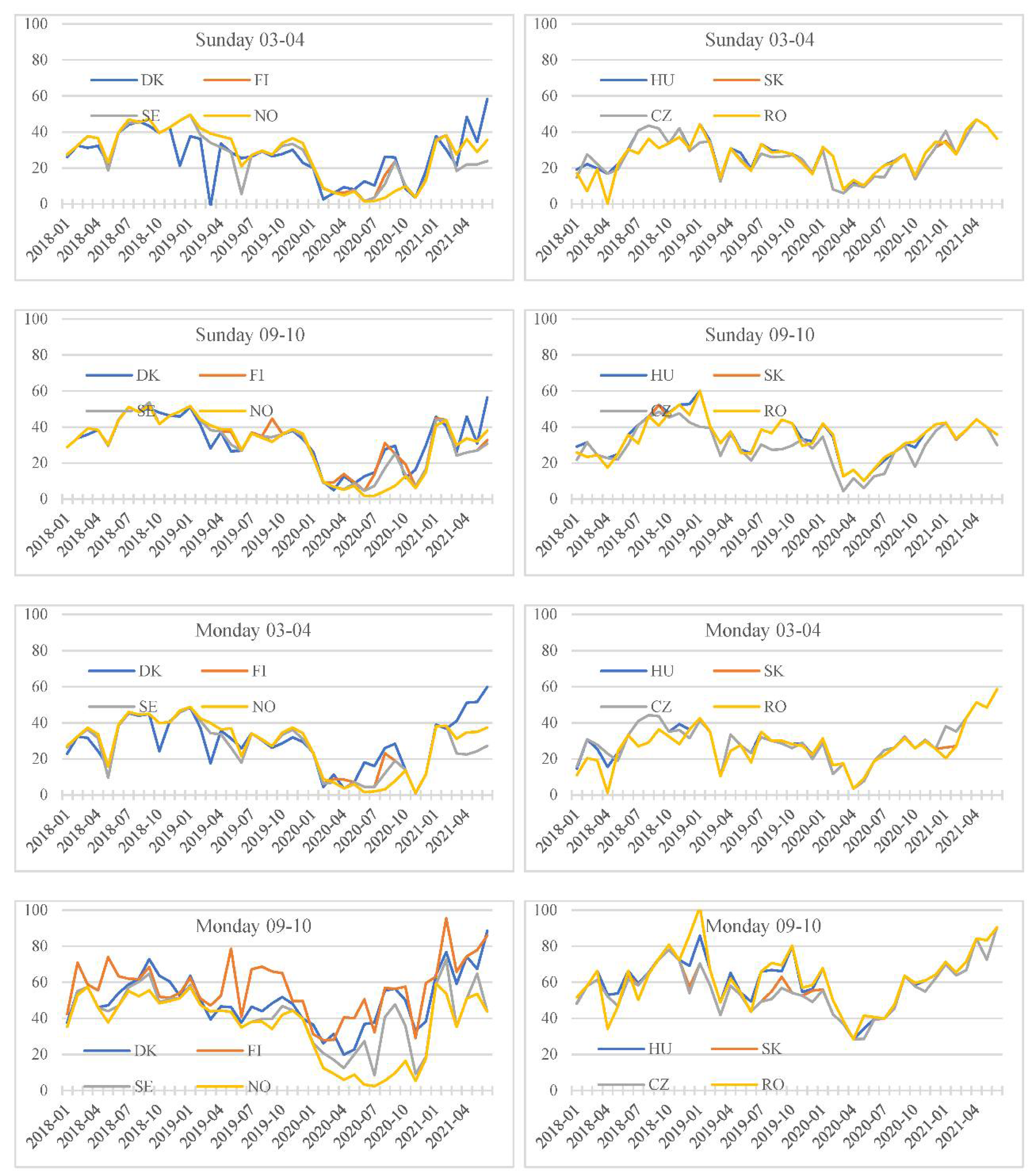
• Sunday, hours between 03–04 and 09–10,
• Monday, hours between 03–04 and 09–10.

The data on energy prices were compared with Eurostat data on the monthly industry output indices in individual countries. As the industry’s output data were related to monthly periods, the energy prices for the individual times were also adopted for these periods, while calculating these as the arithmetic mean of the individual quotations for a given day of the week and an hour in individual months. If a country was divided into several zones for which wholesale energy prices are determined separately, the arithmetic average of the prices of the individual zones was accepted for that country.

Notwithstanding the integration processes, the electricity markets in these countries exhibit a certain nature. There are clear differences in the structure of electricity production (

Table 1. Production of electricity by source, 2020 (in %).

Market	Country	Source
		Fossil Fuels	Nuclear	Wind	Hydro	Biofuels	Solar	Other
Nord Pool	Denmark	15.7	0.0	56.8	0.0	20.6	4.1	2.8
	Finland	13.6	33.9	11.6	23.1	16.8	0.3	0.7
	Sweden	0.5	30.0	16.8	44.2	6.8	0.6	1.1
	Norway	1.3	0.0	6.4	92.0	0.0	0.0	0.3
HUPX	Hungary	37.3	46.2	1.9	0.7	6.2	7.1	0.6
	Slovakia	21.5	53.6	0.0	16.7	5.8	2.3	0.1
	Czechia	48.7	36.9	0.9	4.2	6.4	2.8	0.1
	Romania	34.9	20.5	12.4	28.1	1.0	3.1	0.0

Dark distinction—first share, bright distinction—second share; Source: Eurostat, https://ec.europa.eu/eurostat/cache/infographs/energy/bloc-3b.html?lang=en (accessed on 2 August 2022).

). In general, the countries of the Nord Pool markets are characterised by a significantly higher share of renewable energy, whereas the countries of the HUPX markets have a higher share of fossil energy. Such large differences in the structure of electricity production provide grounds for comparing price sensitivity to fluctuations in the industry’s output.

3. Results

3.1. Variation in Electricity Prices and the Industry’s Output

Wholesale prices on power exchanges are subject to specific short-term fluctuations. Figure 2 shows the development of monthly average prices over the period under study, while

Table 2. Wholesale electricity prices in the markets surveyed.

Statistic	Sunday 03–04
	Denmark	Finland	Sweden	Norway	Hungary	Slovakia	Czechia	Romania
mean	26.79	26.35	26.20	27.82	28.20	26.38	26.51	26.27
st.dev.	13.39	13.63	13.79	14.58	9.93	10.48	10.62	10.36
Statistic	Sunday 09–10
	Denmark	Finland	Sweden	Norway	Hungary	Slovakia	Czechia	Romania
mean	32.64	32.07	30.66	30.41	34.81	30.08	30.00	33.73
st.dev.	12.96	13.26	14.07	15.36	10.94	11.12	10.96	10.71
Statistic	Monday 03–04
	Denmark	Finland	Sweden	Norway	Hungary	Slovakia	Czechia	Romania
mean	29.34	27.04	26.62	28.03	29.54	29.23	29.67	27.06
st.dev.	13.94	13.17	13.60	14.69	11.43	11.32	11.41	11.57
Statistic	Monday 09–10
	Denmark	Finland	Sweden	Norway	Hungary	Slovakia	Czechia	Romania
mean	50.12	56.82	41.65	36.05	61.19	57.04	56.40	61.89
st.dev.	14.56	15.35	15.28	17.87	13.67	13.46	13.37	15.86

presents elementary statistics. The data presented points to clear medium- and short-term price variations, with a strong similarity across the individual national markets; the price trends are consistent. Strong price fluctuations are characteristic of the electricity market, and these occurred here, as well. In peak periods, prices exceeded 40 €/MWh, and in the periods of the greatest downturns they were below 10 €/MWh, and for night hours and Sundays, even below 5 €/MWh. Overall, price variations in all the markets exhibited typical short-term volatility with minima in night periods and on Sundays.

While the variation in prices over time was large, the differentiation between the individual national markets was much smaller. Significant differences were only evident on Mondays for 9–10 o’clock, when prices in the Nord Pool markets, especially in Sweden and Norway, were significantly lower than in the HUPX markets. The average price in relation to this time in the Norwegian market was 36 €/MWh; in the Romanian and Hungarian markets, this exceeded 61 €/MWh. The differences in price levels increased during periods of short-term electricity demand growth.

Prices in the Nord Pool markets prove to be lower on average than in the HUPX markets, yet they are characterised by a higher short-term volatility (a higher standard deviation of electricity prices). This is evident for all the times analysed.

Price variation developments in the individual national markets, especially in the markets of the same exchange, were strongly or very strongly correlated. On the Nord Pool exchange, correlation coefficients ranged from 0.671 for the Denmark–Finland pair (Sunday 03–04) to 0.998 for the Sweden–Finland pair (Sunday 03–04).

Prices in the HUPX markets were even more strongly correlated. Correlation coefficients between monthly average prices ranged from 0.812 for the Czech Republic–Romania pair (Sunday 03–04) to 0.999 for the Czech Republic–Slovakia pair (Sunday 09–10). In general, the correlations between prices in the Czech Republic, Slovakia, and Hungary were very strong (correlation coefficients being above 0.9). The Romanian market was only slightly less linked to the other HUPX markets (correlation coefficients being above 0.8).

Figure 3 and

Table 3. Industry’s output sold index statistics.

Statistic	Nord Pool Country				HUPX Country
	Denmark	Finland	Sweden	Norway	Hungary	Slovakia	Czechia	Romania
mean	103.97	106.93	104.41	99.91	106.73	106.03	101.15	106.57
st.dev.	7.45	7.21	11.39	9.21	11.39	12.97	10.18	12.08

present data on the indexes of the industry’s output sold in each country.

The data presented points to a strong short-term variability in the industry’s output, which is partly due to seasonality. In the Nord Pool markets, especially in Sweden and Norway, production declines were pronounced in July. Average changes in the industry’s output exhibited large differences between the individual countries. Finland, Hungary, Slovakia, and Romania had the highest average of the index, while the Czech Republic and Norway had the lowest average.

From the perspective of the modelling of the relationship between electricity prices and the industry’s output, it is important to retain the trends. In general, the Nord Pool markets saw a slight increase in the value of the indices throughout the period covered by the study, while the HUPX markets saw a decrease in the period up to April 2020, followed by a rapid increase. As with electricity prices, the industry’s output indices in the individual countries were fairly highly correlated with each other. For the countries in the Nord Pool group, correlation coefficients ranged from 0.504 for the Norway–Finland pair to 0.825 for the Denmark–Finland pair. For the countries in the HUPX group, correlation coefficients ranged from 0.859 for the Hungary–Slovakia pair to 0.938 for the Czech Republic–Slovakia pair.

3.2. Model Approach of the Impact of Industry’s Output on Electricity Prices

The core problem of the study concerns the impact of the industry’s output on electricity prices. Two models were built for this relationship:

• a model that shows absolute responses of electricity prices,
• a model that shows relative responses of electricity prices.

The characteristics of the basic parameters of the first model are provided in

Table 4. Model approach of the impact of the industry’s output on electricity prices (prices in EUR/MWh).

Group	Hour		Coef.	S.E.	Conf Int 2.5%	Conf Int 97.5%	z-Ratio	p-Value	VIF	Var (Resid.)	S.E.	IGLS
NORD POOL	Sunday 03–04	β0	28.670	1.231	26.257	31.084	23.284	0.000	1.167	218.32	23.822	1381.61
		β1	0.168	0.122	−0.072	0.408	1.373	0.170
	Sunday 09–10	β0	32.809	1.207	30.444	35.173	27.192	0.000	1.167	209.62	22.872	1374.77
		β1	0.163	0.120	−0.072	0.398	1.358	0.174
	Monday 03–04	β0	29.604	1.193	27.266	31.943	24.811	0.000	1.167	205.00	22.368	1371.03
		β1	0.184	0.119	−0.049	0.416	1.550	0.121
	Monday 09–10	β0	47.775	3.670	40.582	54.968	13.018	0.000	1.019	232.84	25.715	1401.44
		β1	0.241	0.131	−0.015	0.497	1.842	0.065
HUPX	Sunday 03–04	β0	27.017	0.809	25.432	28.602	33.407	0.000	1.184	92.78	10.123	1237.84
		β1	0.327	0.062	0.204	0.449	5.240	0.000
	Sunday 09–10	β0	31.860	0.892	30.111	33.608	35.722	0.000	1.141	89.08	9.838	1232.10
		β1	0.379	0.061	0.259	0.499	6.178	0.000
	Monday 03–04	β0	29.135	0.948	27.277	30.992	30.745	0.000	1.184	127.38	13.899	1291.09
		β1	0.344	0.073	0.201	0.487	4.709	0.000
	Monday 09–10	β0	58.480	0.998	56.523	60.436	58.589	0.000	1.184	141.32	15.420	1308.54
		β1	0.423	0.077	0.273	0.574	5.505	0.000

. Positive correlation coefficients β₁ indicate that in all the countries, an increase in the industry’s output led to an increase in electricity prices. However, fundamental differences in the significance of this response were found. For the Nord Pool countries, the effect of the industry’s output on energy prices on Sunday 03–04, Sunday 09–10, and Monday 03–04 was statistically insignificant, with regression coefficient values oscillating around 0.163–0.184, while on Monday 09–10, the effect could be considered to be close to statistical significance (p = 0.065).

The calculated regression coefficient indicated that a 1 p.p. increase in the industry’s output resulted in a 0.241 €/MWh increase in electricity prices. This is not a significant result, as the confidence interval for this coefficient is (−0.015; 0.497).

For the HUPX countries, the response of electricity prices to variations in the industry’s output was always significant and stronger than for the Nord Pool countries. This is indicated by significantly greater regression coefficients. Their values for Sunday 03–04, Sunday 09–10, and Monday 03–04 were around 0.35 and, for Monday 09–10, they were as high as 0.423. For the Monday peak period, a 1 percentage point increase in the industry’s output resulted in an average increase in electricity prices of 0.423 €/MWh. This quantity may be considered as being very large, given the confidence interval for the regression coefficient (0.273; 0.574).

The second important parameter of the models obtained is the value of free expressions (β₀). They describe the average electricity prices at the value of the industry’s output corresponding to January 2018, taken as a reference point. For Sunday prices and those on Monday 03–04, i.e., the periods of lower prices, these coefficients had slightly lower values for the HUPX group of countries. The differences were within the range of 0.5–1.5 €/MWh. Much greater differences concerned the prices on Monday 09–10, i.e., the high price period. The β0 coefficients calculated for the HUPX countries were significantly greater. They amounted to 58.480, while they were 47.775 for the Nord Pool countries. The difference between the two groups of countries, taken as a whole, was therefore close to 10 €/MWh.

While commenting on the results obtained, it should be noted that the S.E. values of the model parameters for the HUPX countries were always lower than those of the Nord Pool countries. The similarity in the response of electricity prices to variations in the industry’s output in the HUPX countries is therefore greater than that of the Nord Pool countries.

Table 4 also provides the values of the variance inflation factor (VIF), which indicates how much the variance of a coefficient is inflated due to the correlations among the predictors in the model. In the model presented here, a VIF of between 1.019 and 1.184 was obtained, indicating a very weak correlation of the model coefficients, while giving credence to the parameters obtained and their interpretation.

In line with the methodological notes, an analysis was also carried out of the relative responses of electricity prices to variations in the industry’s output. The parameters of this model are provided in

Table 5. Model approach of the impact of the industry’s output on electricity prices (price logarithms).

Group	Hour		Coef.	S.E.	Conf Int 2.5%	Conf Int 97.5%	z-Ratio	p-Value	VIF	Var (Resid.)	S.E.	IGLS
NORD POOL	Sunday 03–04	β0	3.136	0.058	3.023	3.249	54.415	0.000	1.167	0.478	0.052	352.89
		β1	0.013	0.006	0.002	0.025	2.325	0.020
	Sunday 09–10	β0	3.317	0.050	3.219	3.416	65.856	0.000	1.167	0.365	0.040	307.63
		β1	0.012	0.005	0.002	0.022	2.446	0.014
	Monday 03–04	β0	3.188	0.055	3.081	3.296	58.088	0.000	1.167	0.434	0.047	336.43
		β1	0.014	0.005	0.003	0.025	2.565	0.010
	Monday 09–10	β0	3.757	0.109	3.543	3.971	34.355	0.000	1.019	0.214	0.024	226.42
		β1	0.008	0.004	0.000	0.016	2.082	0.037
HUPX	Sunday 03–04	β0	3.221	0.028	3.165	3.276	114.466	0.000	1.184	0.112	0.012	109.41
		β1	0.014	0.002	0.009	0.018	6.228	0.000
	Sunday 09–10	β0	3.402	0.031	3.342	3.463	110.356	0.000	1.108	0.083	0.009	60.52
		β1	0.013	0.002	0.009	0.017	6.933	0.000
	Monday 03–04	β0	3.307	0.033	3.243	3.371	101.176	0.000	1.110	0.095	0.011	83.63
		β1	0.012	0.002	0.008	0.016	5.978	0.000
	Monday 09–10	β0	4.047	0.016	4.016	4.077	259.373	0.000	1.178	0.033	0.004	−93.89
		β1	0.007	0.001	0.005	0.010	6.123	0.000

. The results point to the significance of the impact of variations in the industry’s output for each group of the countries (including the Nord Pool), for each day and hour. Interestingly, the strength of the response for all the countries was similar for all the times analysed. The calculated β₁ coefficients were around 0.012–0.014, so that one percentage point increase in the industry’s output resulted in an increase in electricity prices by ca. 1.2–1.4% on average. A slightly weaker reaction was only found on Mondays 09–10. For the Nord Pool countries, the coefficient was 0.008, and it was 0.007 for the HUPX countries. One percentage point increase in the industry’s output thus caused electricity prices to rise by ca. 0.7–0.8% in this time. In relative terms, the response was therefore weaker, but it related to a time of the day with prices that were significantly higher on average. As with the first model, the S.E. and VIF parameters lend credence to the results obtained and their interpretation.

The differences in the modelling results of the absolute and relative responses of electricity prices to variations in the industry’s output are shown in Figure 4. According to model A (i.e., the absolute response model), higher price levels corresponded to higher absolute increments (combinations: low β₀-low β₁ and high β₀-high β₁). In contrast, according to model B (i.e., the relative response model), higher price levels corresponded to lower relative increments (combinations: low β₀-high β₁ and high β₀-low β₁). Thus, with high prices, one may speak of high absolute volatility but low relative volatility; conversely, with low prices, one may speak of low absolute volatility but high relative volatility.

The models presented above show aggregate results for the two groups of countries. The subject of interest was whether and to what extent the individual country responses within the two groups were similar. The results for the individual countries based on the modelling of relative responses (model B) are shown in Figure 5.

The results obtained point to divergences between the groups of the countries studied. The results presented in Table 5 indicate that all the responses were statistically significant, but the observation of S.E. values for the model parameters allows one to consider that the results for the HUPX countries were more stable and less differentiated than for the Nord Pool countries. Consequently, the individual regression lines shown in Figure 5 for the HUPX countries were very similar, while those for the Nord Pool countries exhibited greater differences. Overall, therefore, the responses of electricity prices to variations in the industry’s output for the HUPX countries exhibited great similarity. In contrast, there was greater national specificity for the Nord Pool countries. Of this group, Finland had the flattest regression line (a weak response of electricity prices to the industry’s output sold).

4. Conclusions

The analyses were carried out in order to determine whether and to what extent variations in the industry’s output influence changes in electricity prices. In addition, attempts were made to determine whether, if confirmed, this impact varies depending on periods with different levels of electricity demand and, consequently, electricity prices, as well as on the groups of countries. In this respect, this research supplements the knowledge on the formation of electricity prices and may be important in the line of the state’s energy policy.

The Nord Pool and HUPX exchanges bring together different countries with specificities in terms of their energy mixes. In general, the Nord Pool countries have more diversified electricity sources, with a high share of renewable energy. In the HUPX countries, the vast majority of energy came from fossil fuels and nuclear power. This meant that prices within individual power exchanges were similar and strongly correlated, while greater differences occurred between groups of countries. Despite the prevalence of common global factors affecting energy prices, it is local conditions (tax regimes, energy sources, as well as local supply and demand) that play an important role in the formation of electricity prices. Lower wholesale prices were characteristic of the Nord Pool markets, with a higher share of renewable energy. This shows that energy transformation can be an important factor in stabilizing the electricity market.

The results of the study unambiguously allow one to recognise variations in the industry’s output sold as a significant determinant in the formation of electricity prices. Thus, hypothesis H1 was positively verified. For each power exchange, and for each country, an increase in the industry’s output sold translated into an increase in electricity prices. Moreover, the relative strength of the response for each country was similar.

However, the results obtained do not give grounds for hypotheses H2 and H3 to be accepted. Variations in the industry’s output had a similar effect on price increases in the periods of low demand and lower energy prices (Sunday, night hours) and the periods of high demand (Monday, 09–10). An increase in the industry’s output has a positive effect on electricity price levels, yet this does not increase the disparities between prices on days/at times of high and low energy consumption.

Likewise, hypothesis H3 may not be confirmed unequivocally. Admittedly, the absolute responses in the HUPX markets with a high share of fossil fuel energy were stronger than in the case of the Nord Pool markets with a high share of renewable energy. The structure of electricity production by energy source may have an impact on the average price level, but not on its sensitivity to a change in demand conditions resulting from a variation in the industry’s output. However, it should be noted that the present study does not analyse whether and to what extent changes in the share of electricity from renewable sources affect the energy price level and the price response to variations in the industry’s output. Taking into account this dynamic aspect of changes in the structure of electricity production could allow for a more precise verification of hypothesis H3.

References

1. Safa, H. The impact of energy on global economy. Int. J. Energy Econ. Policy 2017, 7, 287–295. [Google Scholar]
2. Wu, X.F.; Chen, G.Q. Global primary energy use associated with production, consumption and international trade. Energy Policy 2017, 111, 85–94. [Google Scholar] [CrossRef]
3. Cass, D. Optimum growth in an aggregative model of capital accumulation. Rev. Econ. Stud. 1965, 32, 233–240. [Google Scholar] [CrossRef] [Green Version]
4. Koopmans, T.C. Objectives, constraints, and outcomes in optimal growth models. Econometrica 1967, 35, 110–132. [Google Scholar] [CrossRef]
5. Cleveland, C.J.; Kaufmann, R.K.; Stern, D.I. Aggregation and the role of energy in the economy. Ecol. Econ. 2000, 32, 301. [Google Scholar] [CrossRef]
6. Ayres, R.U.; Warr, B. Accounting for growth: The role of physical work. Struct. Chang. Econ. Dyn. 2005, 16, 181–209. [Google Scholar] [CrossRef]
7. Van de Ven, D.J.; Fouquet, R. Historical energy prices and their changing effect on the economy. Energy Econ. 2017, 62, 204–216. [Google Scholar] [CrossRef] [Green Version]
8. Lee, K.; Ni, S.; Ratti, R. Oil shocks and the macroeconomy: The role of price variability. Energy J. 1995, 16, 39–56. [Google Scholar] [CrossRef] [Green Version]
9. Barsky, R.B.; Kilian, L. Do we really know that oil caused the great stagflation? A monetary alternative. NBER Macroecon. Annu. 2011, 16, 137–183. [Google Scholar] [CrossRef]
10. Bernanke, B.; Gertler, M.; Watson, M. Systematic monetary policy and the effect of oil price shocks. Brook. Pap. Econ. Act. 1997, 1, 91–142. [Google Scholar] [CrossRef] [Green Version]
11. Hunt, R.; Isard, P.; Laxton, D. The macroeconomic effects of higher oil prices. Natl. Inst. Econ. Rev. 2002, 179, 87–103. [Google Scholar] [CrossRef]
12. Bildirici, M.; Alp, E.A.; Bakirtas, T. The great recession and the effects of oil price shocks and the U.S. recession: A Markov-switching and TAR-VEC analysis. J. Energy Dev. 2011, 35, 215–277. [Google Scholar]
13. Burbidge, J.; Harrison, A. Testing for the effects of oil-price using vector autoregressions. Int. Econ. Rev. 1984, 25, 459–484. [Google Scholar] [CrossRef]
14. Mork, K.A.; Olsen, O.; Mysen, H.T. Macroeconomic responses to oil price increases and decreases in seven OECD countries. Energy J. 1994, 15, 19–35. [Google Scholar]
15. Ewing, B.T.; Sari, R.; Soytas, U. Disaggregate energy consumption and industrial output in the United States. Energy Policy 2007, 35, 1274–1281. [Google Scholar] [CrossRef]
16. Kilian, L. The economic effects of energy price shocks. J. Econ. Lit. 2008, 46, 871–909. [Google Scholar] [CrossRef] [Green Version]
17. Lee, C.C. The causality relationship between energy consumption and GDP in G-11 countries revisited. Energy Policy 2006, 34, 1086–1093. [Google Scholar] [CrossRef]
18. Narayan, P.K.; Smyth, R. Electricity consumption, employment and real income in Australia evidence from multivariate Granger causality tests. Energy Policy 2005, 33, 1109–1116. [Google Scholar] [CrossRef]
19. Erol, U.; Yu, E.S. On the causal relationship between energy and income for industrialized countries. J. Energy Dev. 1987, 13, 113–122. [Google Scholar]
20. Stern, D.I. A multivariate cointegration analysis of the role of energy in the US macroeconomy. Energy Econ. 2000, 22, 267–283. [Google Scholar] [CrossRef] [Green Version]
21. Thoma, M. Electrical energy usage over the business cycle. Energy Econ. 2004, 26, 463–485. [Google Scholar] [CrossRef]
22. Mir, A.A.; Alghassab, M.; Ullah, K.; Khan, Z.A.; Lu, Y.; Imran, M. A review of electricity demand forecasting in low and middle income countries: The demand determinants and horizons. Sustainability 2020, 12, 5931. [Google Scholar] [CrossRef]
23. Weron, R. Electricity price forecasting. a review of the state-of-the-art with a look into the future. Int. J. Forecast. 2014, 30, 1030–1081. [Google Scholar] [CrossRef] [Green Version]
24. Härdle, W.K.; Trück, S. The Dynamics of Hourly Electricity Prices; SFB 649 Discussion Paper 2010–013. 2010. Available online: https://papers.ssrn.com/sol3/papers.cfm?abstract_id=2894267 (accessed on 1 August 2022).
25. McCulloch, J.; Ignatieva, K. Intra-day electricity demand and temperature. Energy J. 2020, 41, 161–181. [Google Scholar] [CrossRef]
26. Karakatsani, N.V.; Bunn, D.W. Forecasting electricity prices: The impact of fundamentals and time-varying coefficients. Int. J. Forecast. 2008, 24, 764–785. [Google Scholar] [CrossRef]
27. Fanone, E.; Gamba, A.; Prokopczuk, M. The case of negative Day-ahead electricity prices. Energy Econ. 2013, 35, 22–34. [Google Scholar] [CrossRef]
28. Huisman, R.; Huurman, C.; Mahieu, R. Hourly electricity prices in day-ahead markets. Energy Econ. 2007, 29, 240–248. [Google Scholar] [CrossRef] [Green Version]
29. Christensen, T.M.; Hurn, A.S.; Lindsay, K.A. Forecasting spikes in electricity prices. Int. J. Forecast. 2012, 28, 400–411. [Google Scholar] [CrossRef]
30. Negrete-Pincetic, M.; de Castro, L.; Pulgar-Painemal, H.A. Electricity Supply Auctions: Understanding the Consequences of the Product Definition. Electr. Power Energy Syst. 2015, 64, 285–292. [Google Scholar] [CrossRef]
31. Zachmann, G. Electricity wholesale market prices in Europe: Convergence? Energy Econ. 2008, 30, 1659–1671. [Google Scholar] [CrossRef]
32. Pellini, E. Convergence across European Electricity Wholesale Spot Markets: Still a Way to Go. Essays on European Electricity Market Integration. Ph.D. Thesis, University of Surrey, Guildford, UK, 2014; pp. 100–132. [Google Scholar]
33. Figueiredo, N.C.; da Silva, P.P. The “Merit-order effect” of wind and solar power: Volatility and determinants. Renew. Sustain. Energy Rev. 2019, 102, 54–62. [Google Scholar] [CrossRef]
34. Sensfuß, F.; Ragwitz, M.; Genoese, M. The merit-order effect: A detailed analysis of the price effect of renewable electricity generation on spot market prices in Germany. Energy Policy 2008, 36, 3086–3094. [Google Scholar] [CrossRef] [Green Version]
35. Moselle, B.; Padilla, J.; Schmalensee, R. Harnessing Renewable Energy in Electric Power Systems: Theory, Practice, Policy; Earthscan, Routledge: New York, NY, USA, 2010. [Google Scholar]
36. Hox, J.J. Multilevel Analysis: Techniques and Applications; Erlbaum: Mahwah, NJ, USA, 2002. [Google Scholar]
37. Bryk, A.S.; Raudenbush, S.W. Hierarchical Linear Models; Sage: Newbury Park, CA, USA, 1992. [Google Scholar]
38. Mass, J.; Hox, J.J. The Influence of Violations of Assumptions on Multilevel Parameter Estimates and Their Standard Errors. Comput. Stat. Data Anal. 2003, 46, 427–440. [Google Scholar] [CrossRef]
39. El-Horbaty, Y.S.; Hanafy, E.M. Some Estimation Methods and Their Assessment in Multilevel Models: A Review. Biostat. Biom. Open Access J. 2018, 5, 555662. [Google Scholar] [CrossRef]
40. Goldstein, H. Multilevel Mixed Linear Model Analysis Using Iterative Generalized Least-Squares. Biometrika 1986, 73, 43–56. [Google Scholar] [CrossRef]
41. Goldstein, H. Multilevel Statistical Models; Institute of Education: London, UK, 1995. [Google Scholar]
Figure 1. Two-level data structure.
Energies 15 06044 g001
Figure 2. Stock exchange prices of electricity (EUR/MWh).
Energies 15 06044 g002
Figure 3. Indexes of the industry’s output sold (January 2018 = 100).
Energies 15 06044 g003
Figure 4. Relationship between β0 and β1 parameters in individual models.
Energies 15 06044 g004
Figure 5. Individual relationship between logarithms of electricity prices and rates of the industry’s output.
Energies 15 06044 g005