
Assessment of Turbulence Models over a Curved Hill Flow with Passive Scalar Transport


Abstract
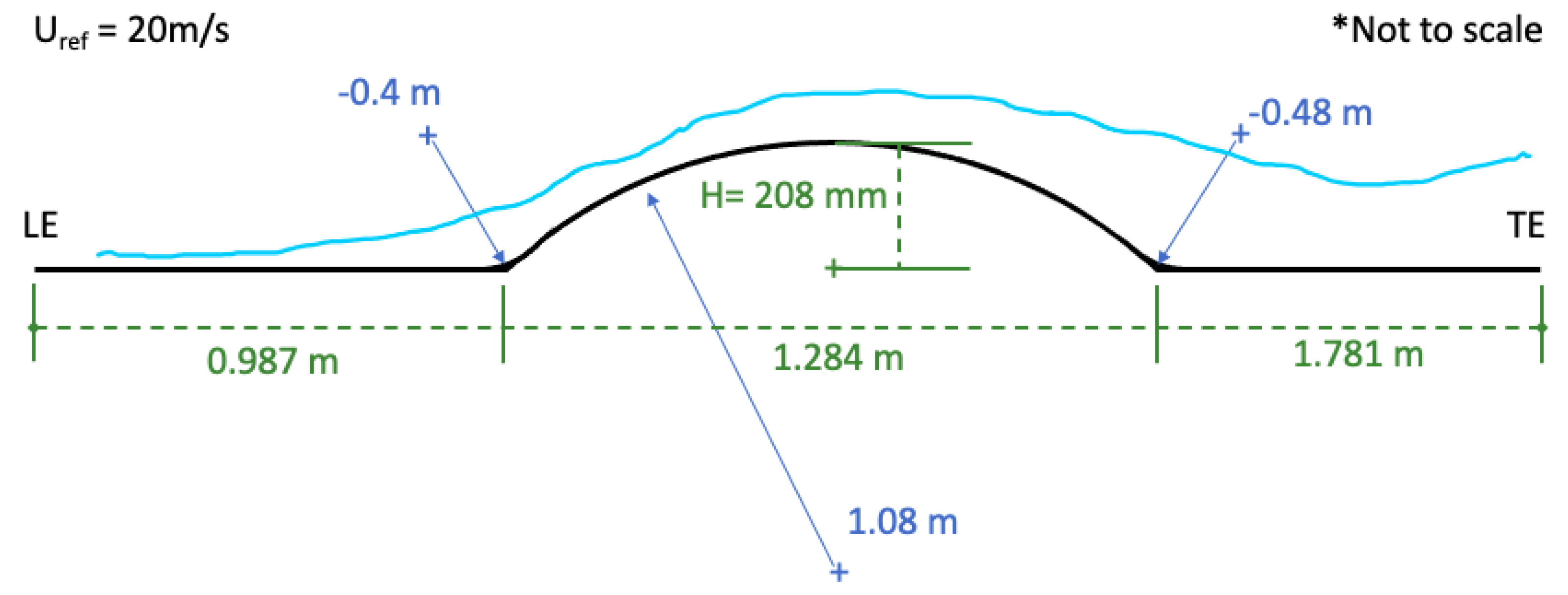
:1. Introduction
1.1. Scope of the Present Work
1.2. Background
2. Formulations
2.1. Reynolds Averaged Navier–Stokes Equation
2.2. Turbulent Flow Models
2.3. Flow Solver and Numerical Schemes
2.4. Boundary Layer Detection Based on Potential Flow
2.5. Turbulent Inflow Generation
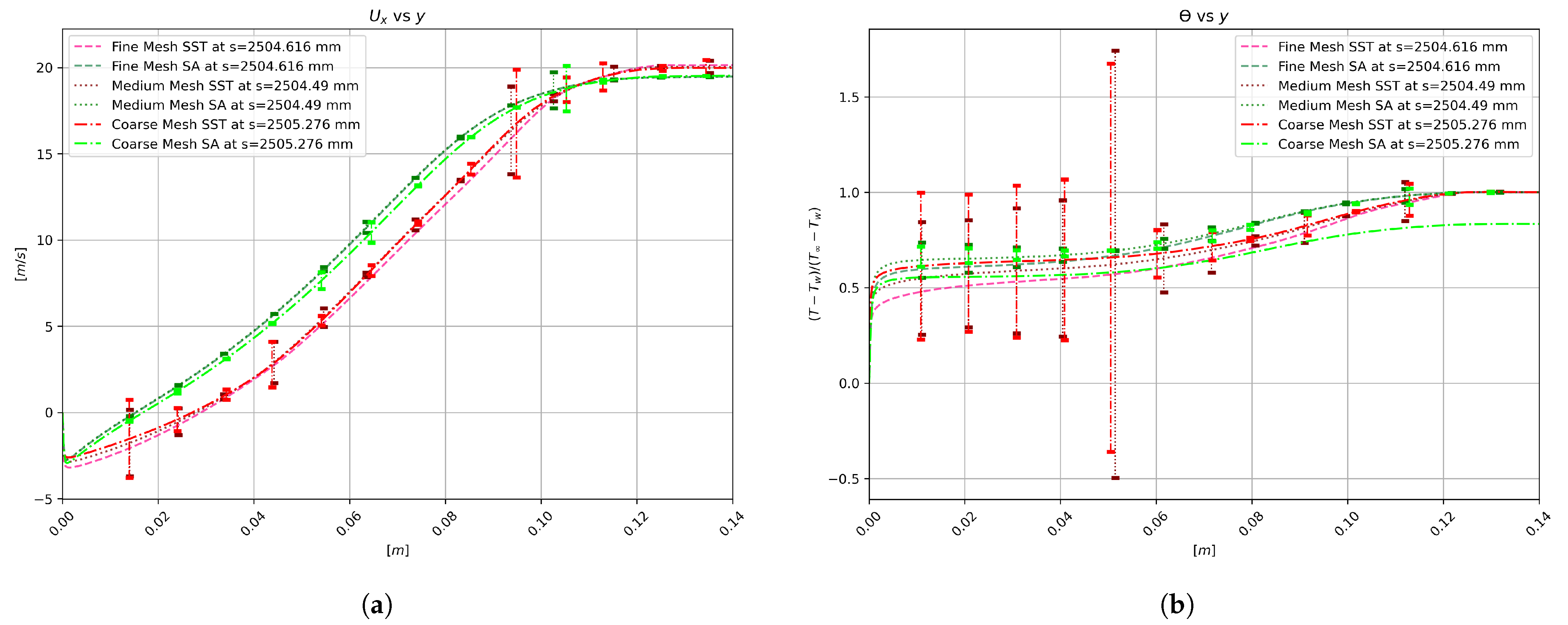
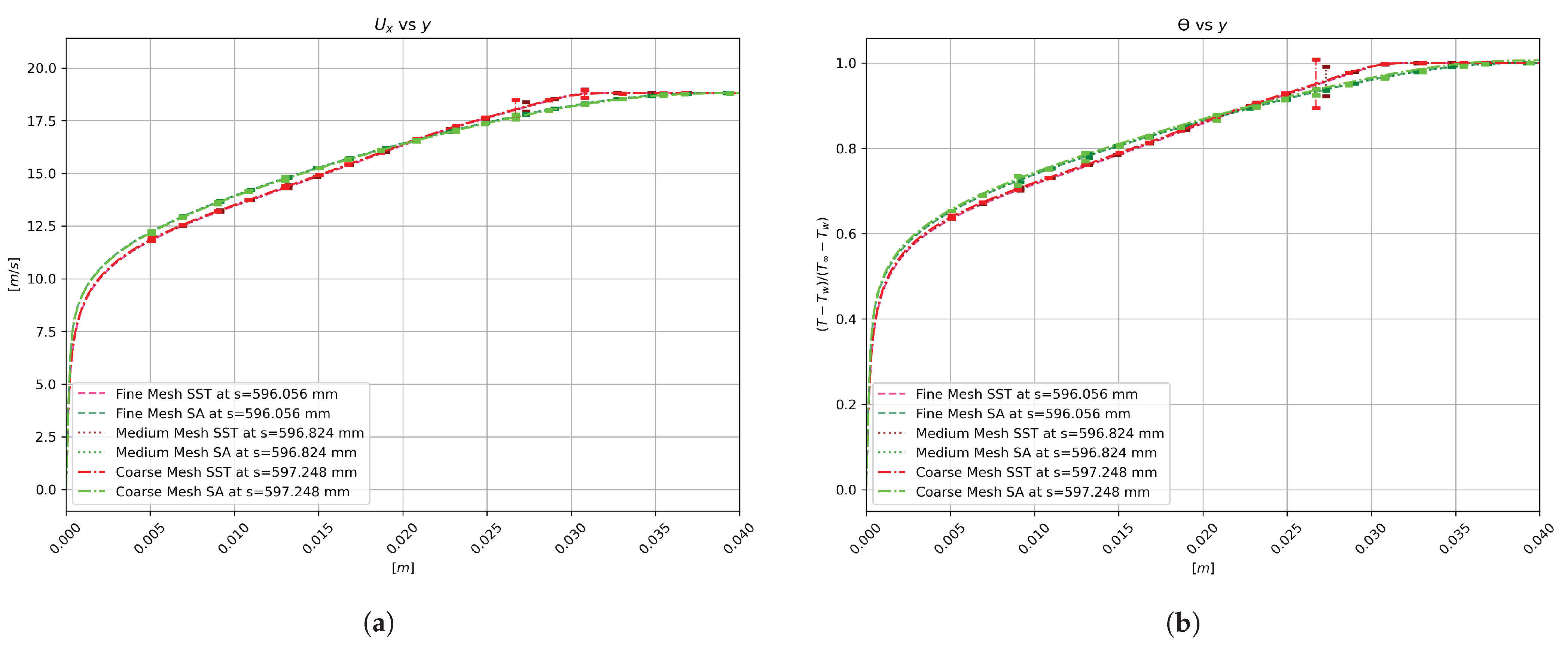
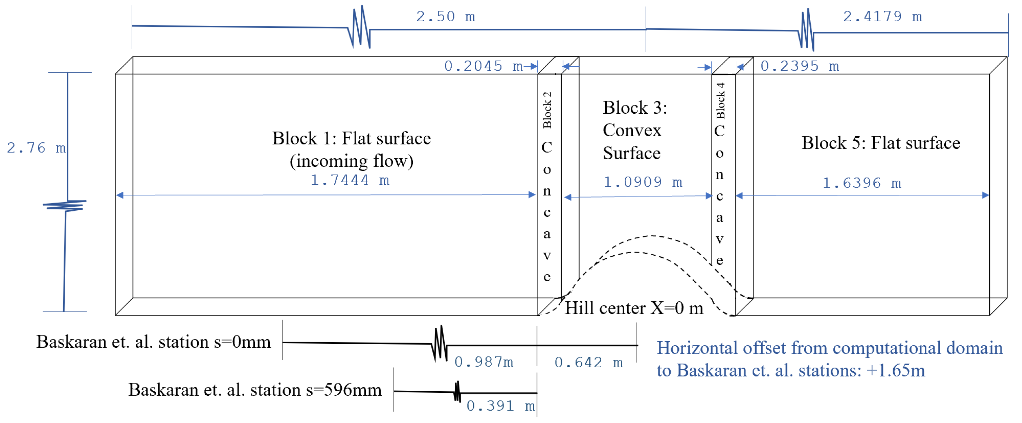
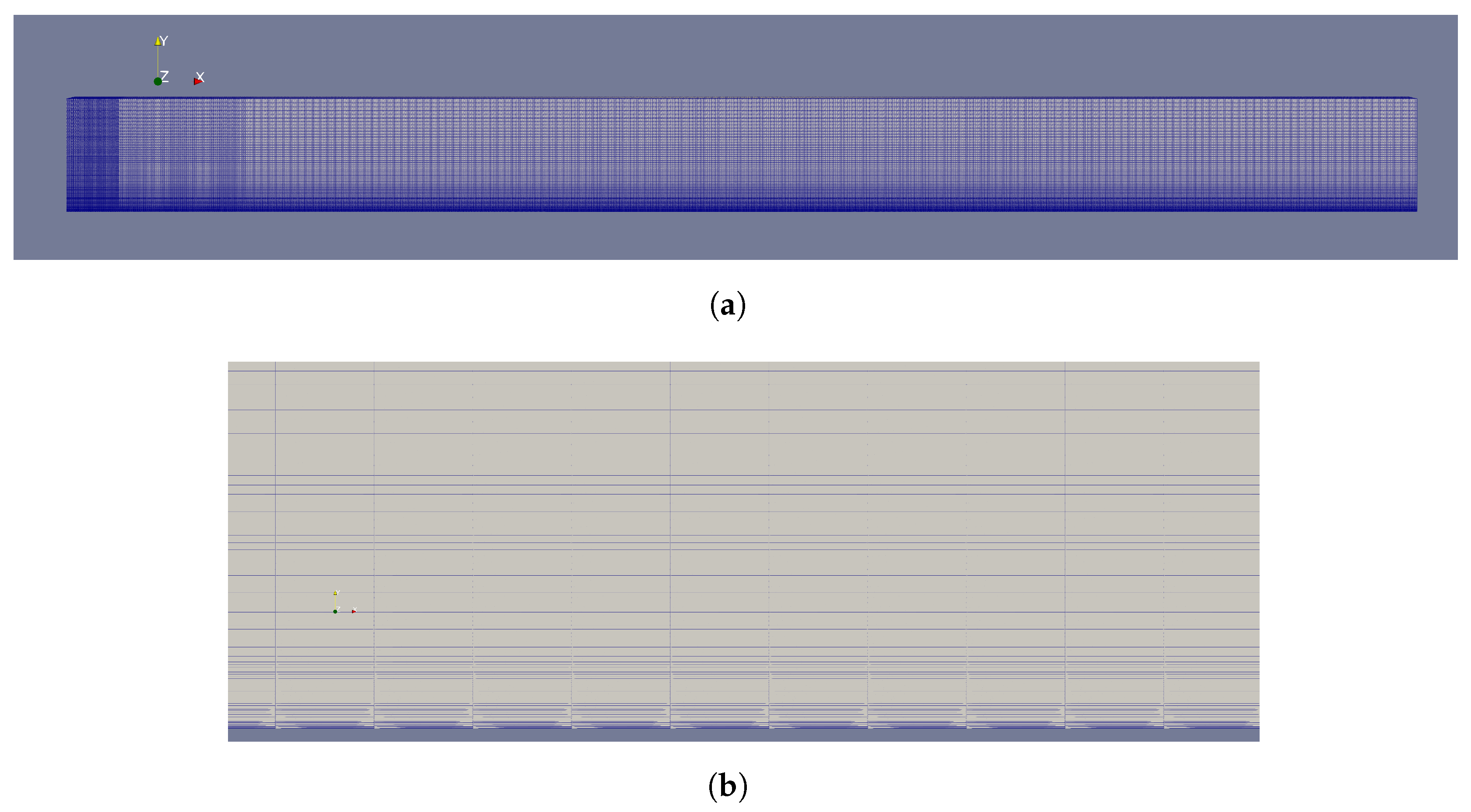
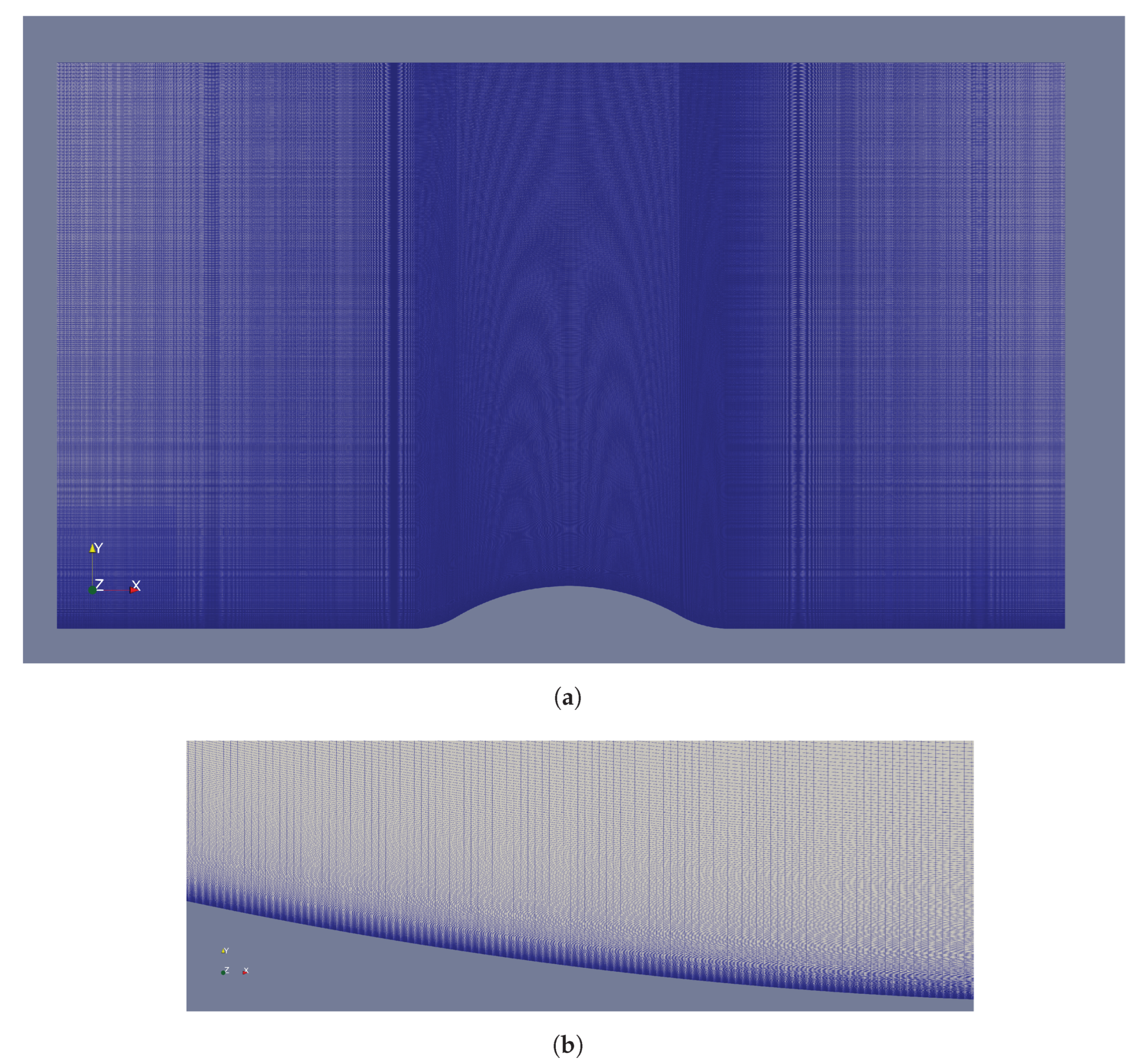
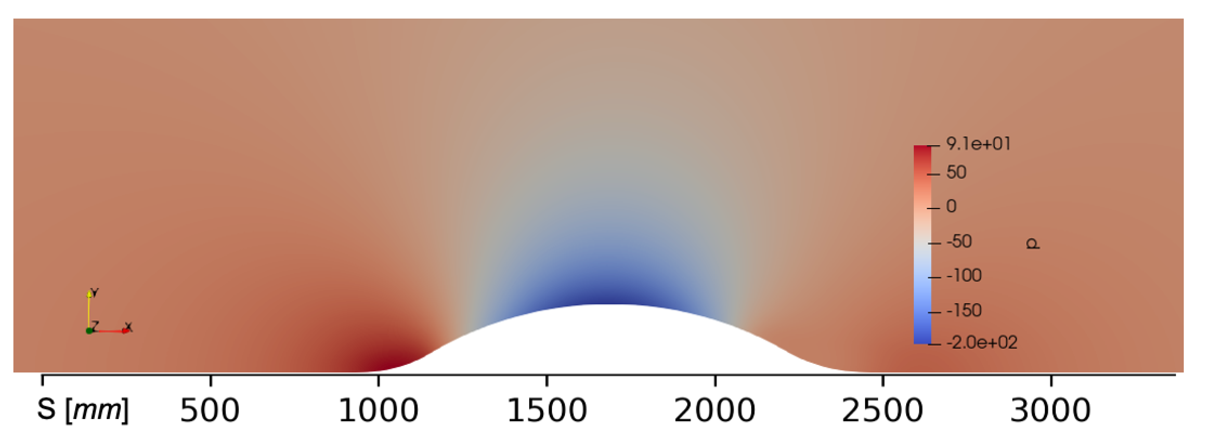
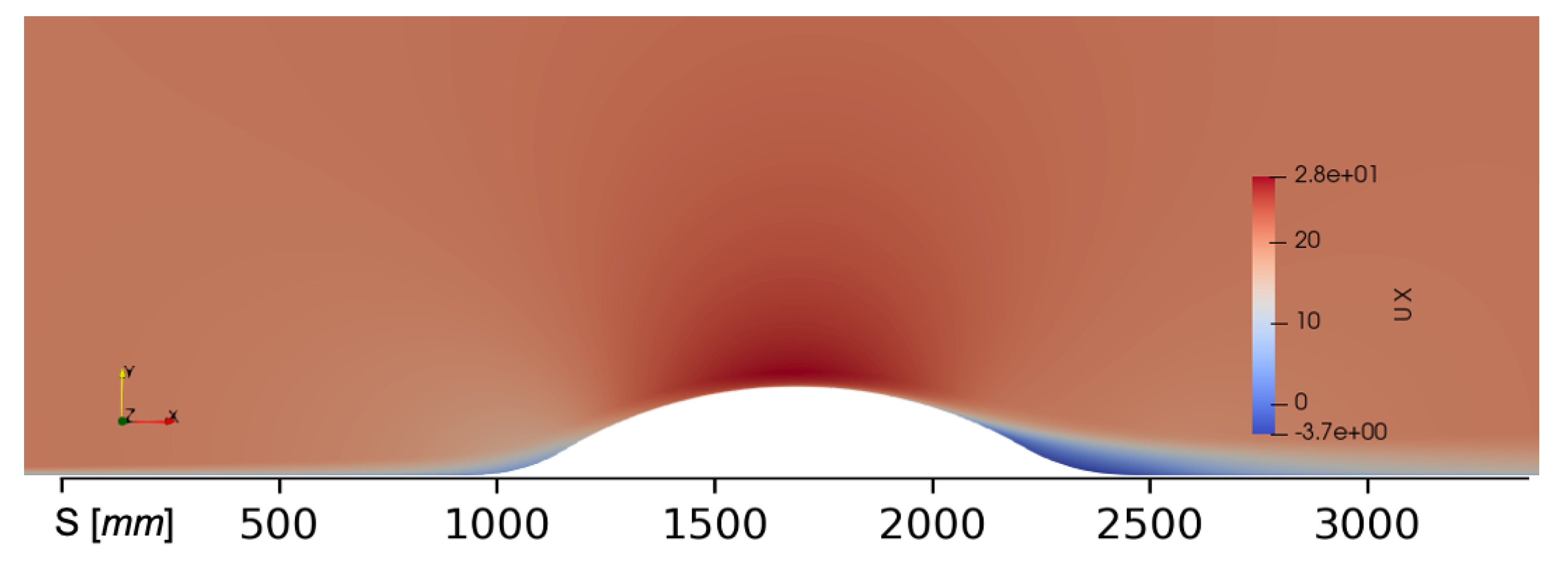
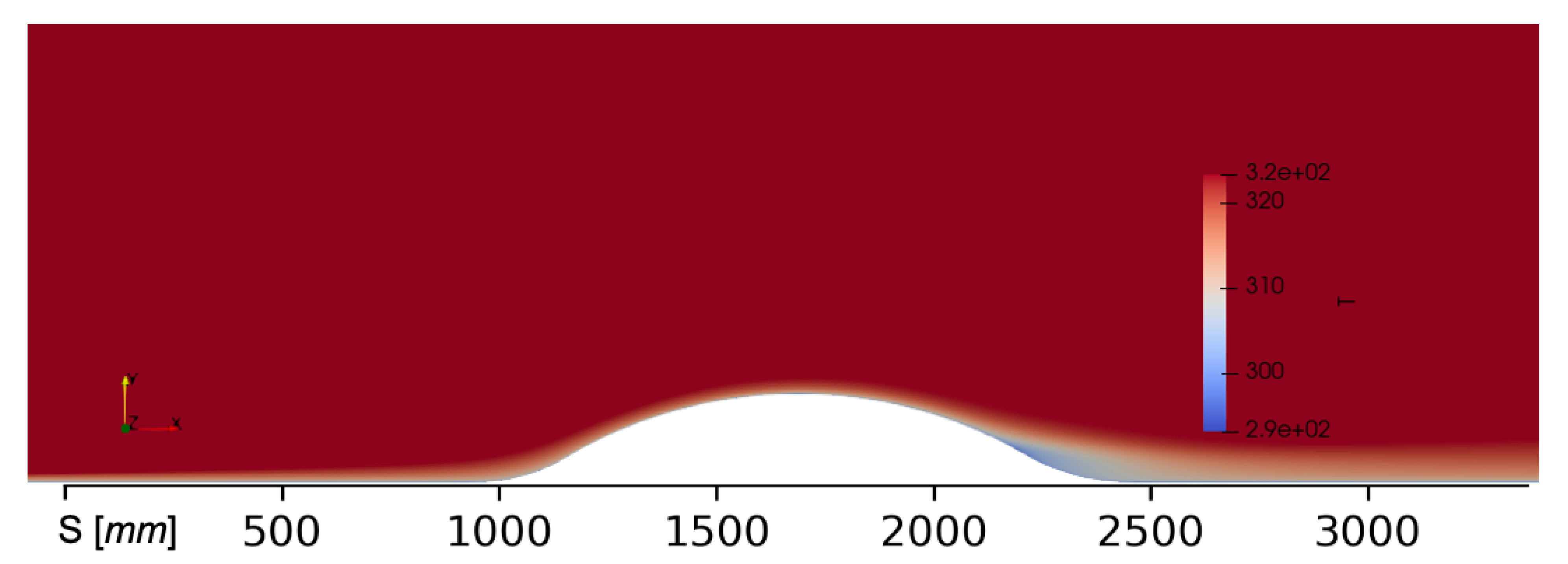
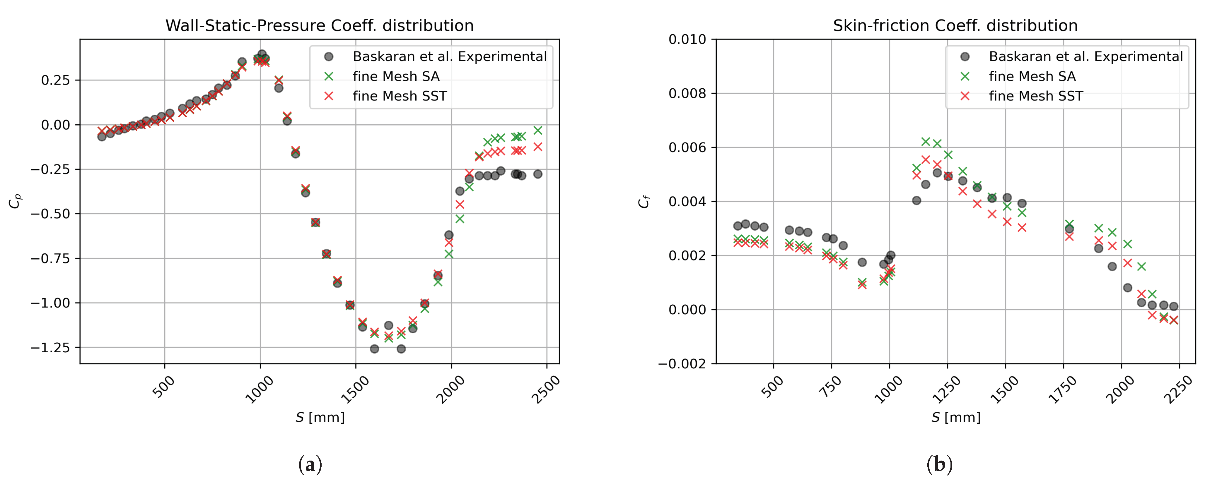
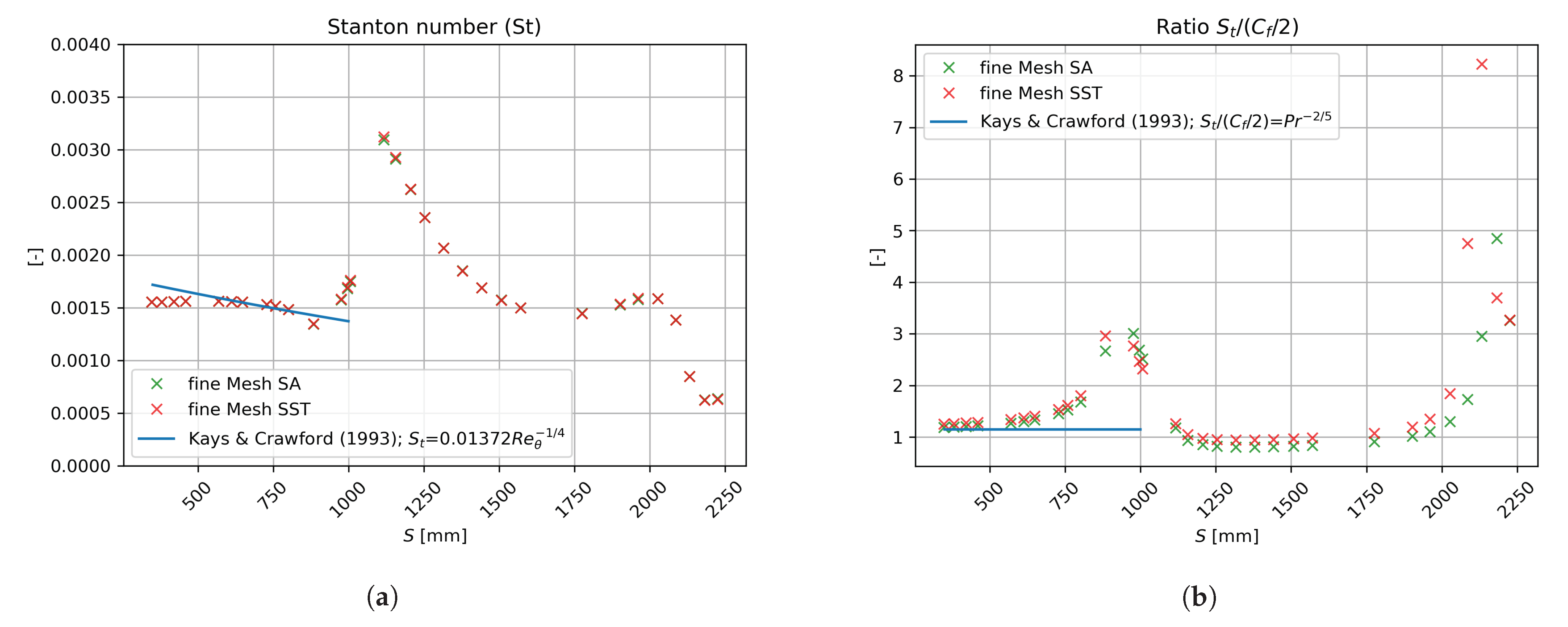
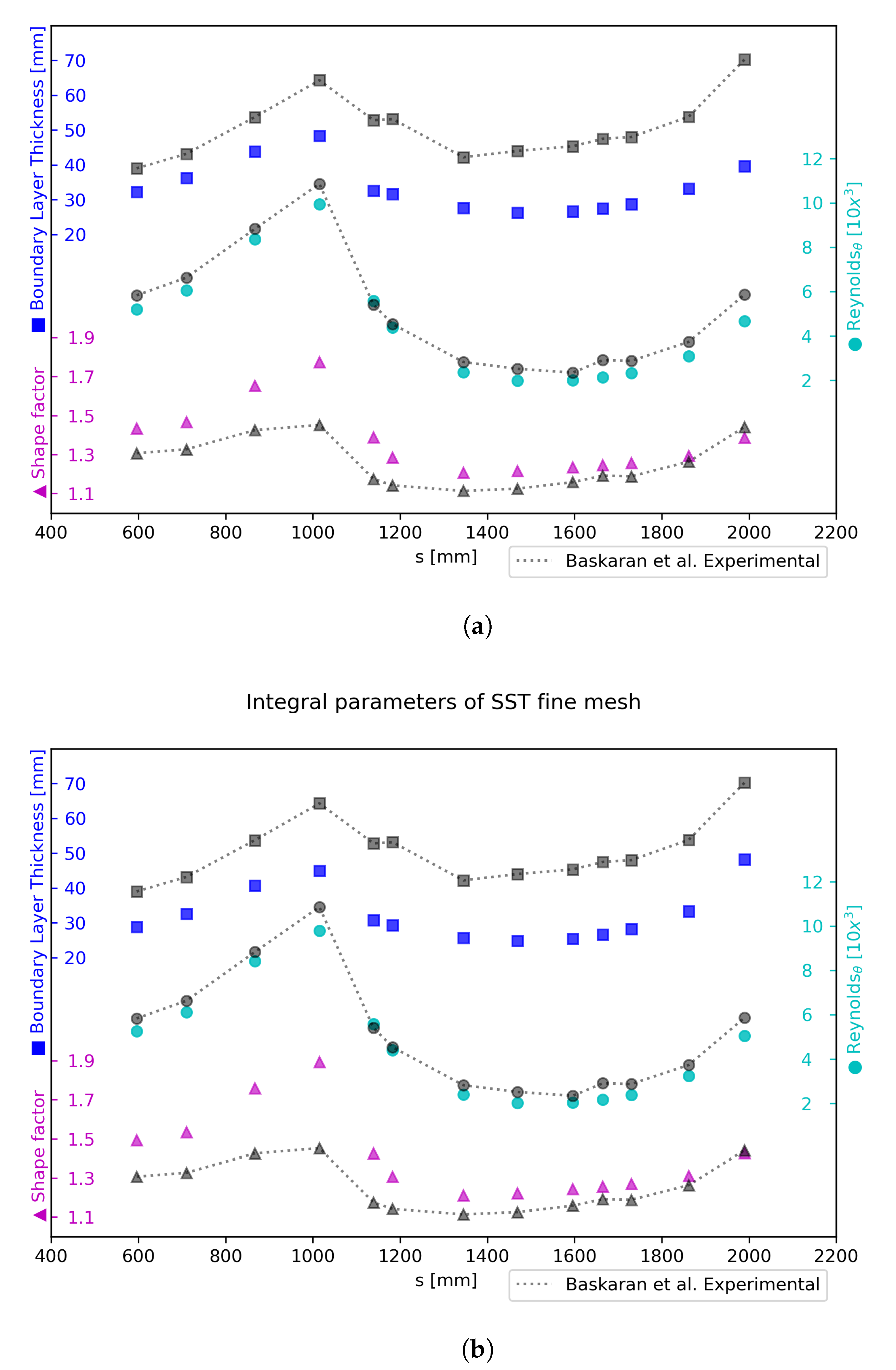
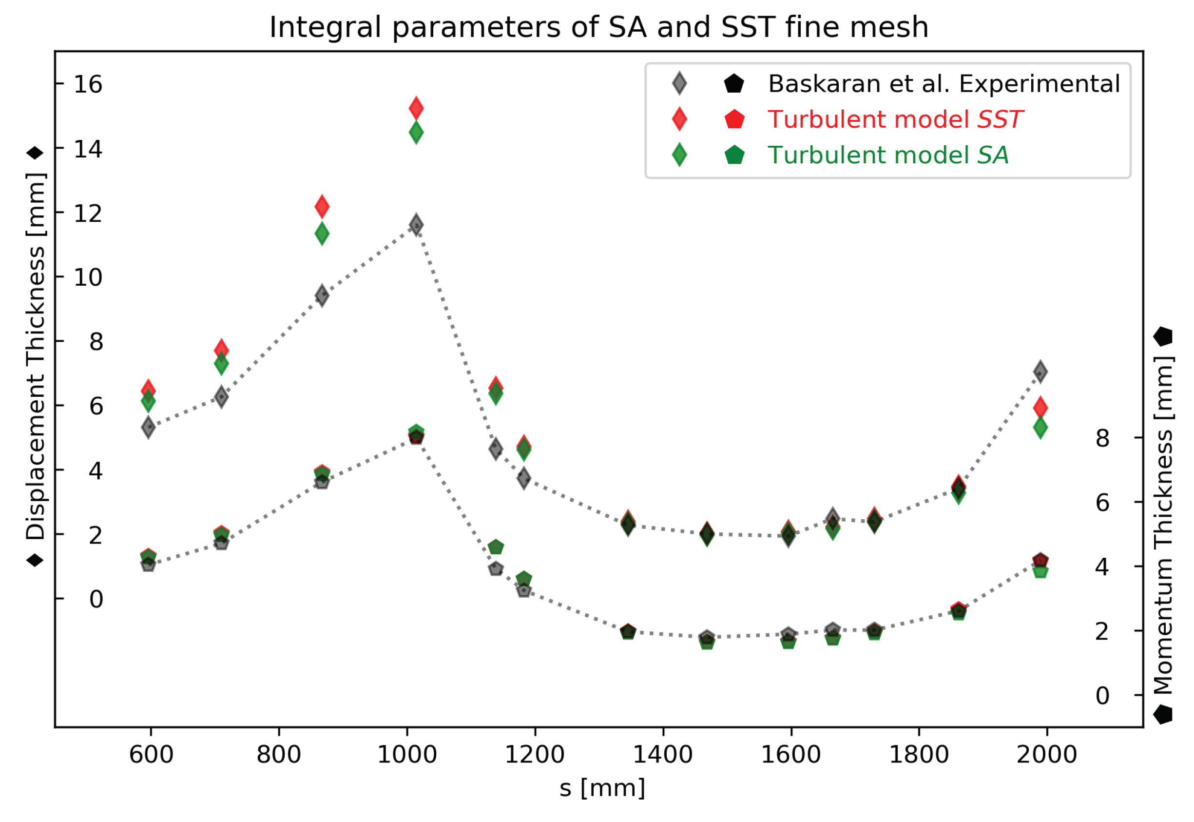
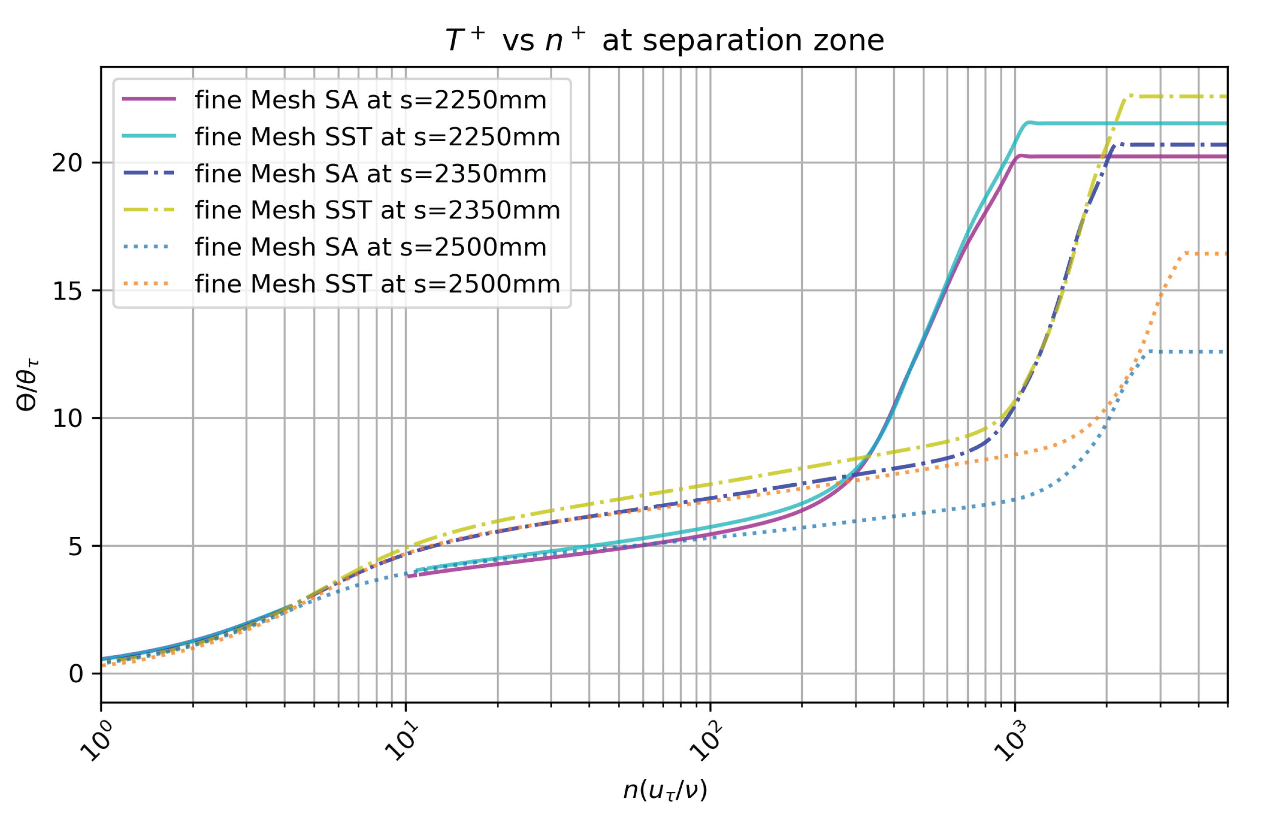
3. Numerical Results and Discussion for the Curved Hill
4. Conclusions
Author Contributions
Funding
Institutional Review Board Statement
Informed Consent Statement
Data Availability Statement
Acknowledgments
Conflicts of Interest
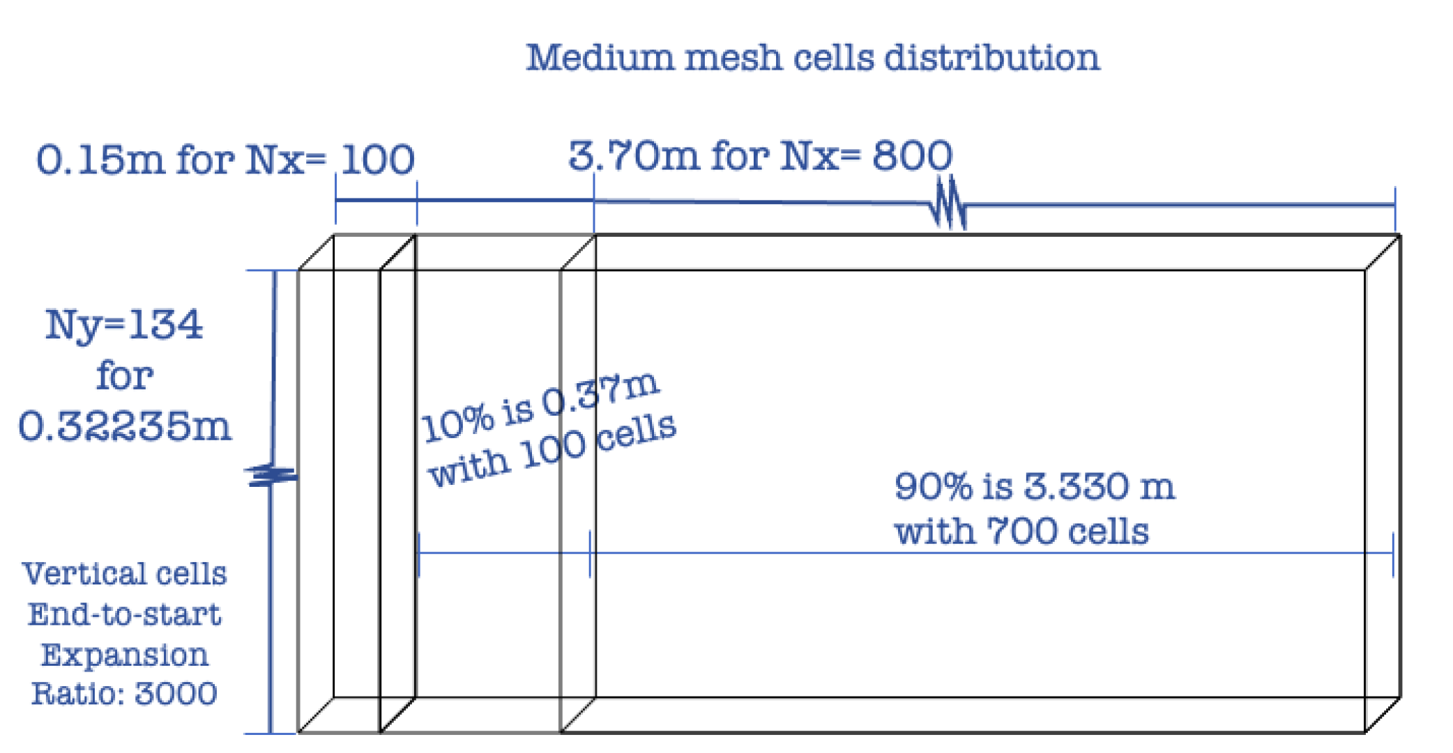
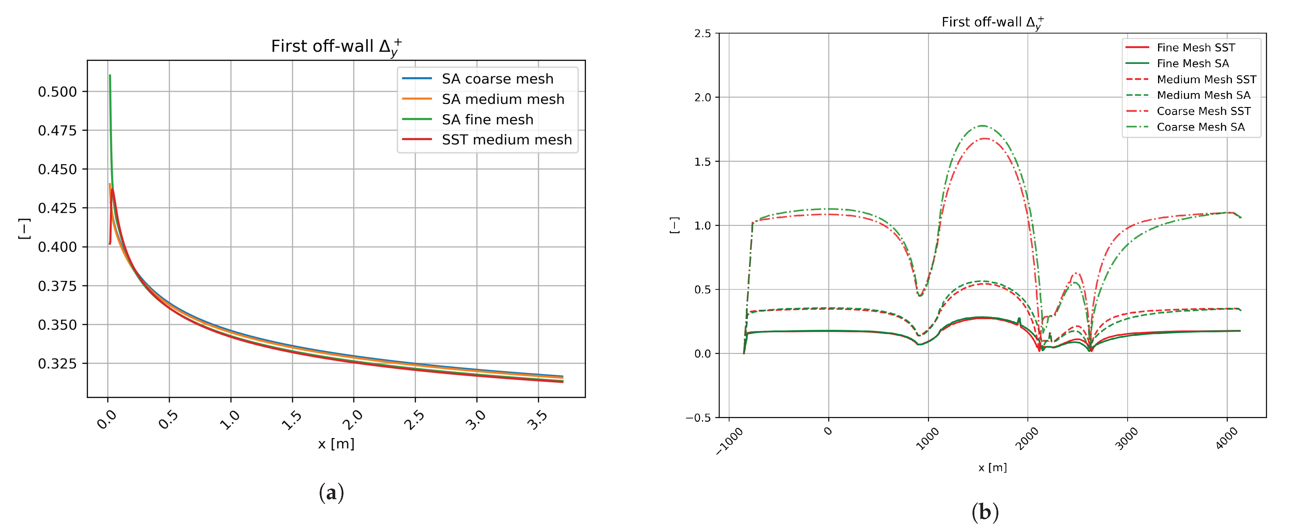
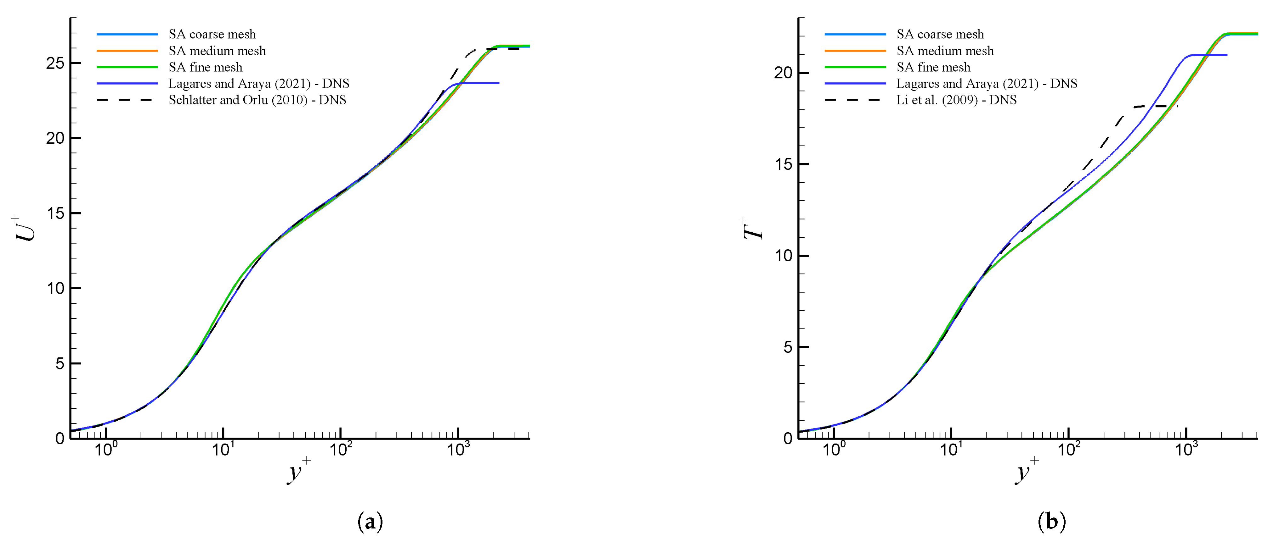
Appendix A. Grid Sensitivity Study

| Stations (mm) | 596 | 710 | 867 | 1015 | 1139 | 1183 | 1345 | 1469 | 1596 | 1665 | 1730 | 1862 | 1990 |
| Experimental (mm) | 5.3108 | 6.2568 | 9.3987 | 11.5946 | 4.6352 | 3.7230 | 2.2703 | 2.0000 | 1.9325 | 2.4730 | 2.3716 | 3.4189 | 7.0338 |
| SST fine mesh (mm) | 6.4351 | 7.6986 | 12.1624 | 15.2198 | 6.5256 | 4.7115 | 2.3776 | 2.0155 | 2.0727 | 2.2290 | 2.4768 | 3.4724 | 5.9165 |
| SST medium mesh (mm) | 6.3852 | 7.6428 | 12.1447 | 15.1597 | 6.0952 | 4.6767 | 2.3269 | 1.9677 | 2.0225 | 2.1779 | 2.4090 | 3.3711 | 5.8081 |
| SST coarse mesh (mm) | 6.3403 | 7.5589 | 12.0473 | 15.2093 | 6.5252 | 4.6499 | 2.2817 | 1.9098 | 1.9505 | 2.1029 | 2.3374 | 3.2521 | 5.5843 |
| Rel. Error (fine to exp.) | 19.14% | 20.66% | 25.64% | 27.04% | 33.88% | 23.44% | 4.62% | 0.77% | 7.01% | −10.38% | 4.34% | 1.55% | −17.26% |
| Rel. Error (medium to fine) | −0.78% | −0.73% | −0.15% | −0.40% | −6.82% | −0.74% | −2.16% | −2.40% | −2.45% | −2.32% | −2.78% | −2.96% | −1.85% |
| Rel. Error (coarse to medium) | −0.71% | −1.10% | −0.80% | 0.33% | 6.81% | −0.57% | −1.96% | −2.99% | −3.63% | −3.50% | −3.02% | −3.59% | -3.93% |
| Experimental (mm) | 5.3108 | 6.2568 | 9.3987 | 11.5946 | 4.6352 | 3.7230 | 2.2703 | 2.0000 | 1.9325 | 2.4730 | 2.3716 | 3.4189 | 7.0338 |
| SA fine mesh (mm) | 6.1274 | 7.2940 | 11.3322 | 14.4704 | 6.3664 | 4.6301 | 2.3285 | 1.9750 | 2.0251 | 2.1694 | 2.3982 | 3.2684 | 5.3129 |
| SA medium mesh (mm) | 6.1019 | 7.2670 | 11.3463 | 14.3841 | 5.9822 | 4.6167 | 2.3026 | 1.9526 | 2.0026 | 2.1372 | 2.3769 | 3.2297 | 5.3106 |
| SA coarse mesh (mm) | 6.1584 | 7.3110 | 11.4325 | 14.6143 | 6.4907 | 4.6748 | 2.3088 | 1.9493 | 2.0002 | 2.1509 | 2.3815 | 3.2517 | 5.3431 |
| Rel. Error (fine to exp.) | 14.28% | 15.31% | 18.65% | 22.07% | 31.47% | 21.72% | 2.53% | −1.26% | 4.68% | −13.08% | 1.11% | −4.50% | −27.88% |
| Rel. Error (medium to fine) | −0.42% | −0.37% | 0.12% | −0.60% | −6.22% | −0.29% | −1.12% | −1.14% | −1.12% | −1.49% | −0.89% | −1.19% | −0.04% |
| Rel. Error (coarse to medium) | 0.92% | 0.60% | 0.76% | 1.59% | 8.15% | 1.25% | 0.27% | −0.17% | −0.12% | 0.64% | 0.19% | 0.68% | 0.61% |
| Stations (mm) | 596 | 710 | 867 | 1015 | 1139 | 1183 | 1345 | 1469 | 1596 | 1665 | 1730 | 1862 | 1990 |
| SST fine mesh (mm) | 4.3102 | 5.0204 | 6.9113 | 8.0405 | 4.5770 | 3.6047 | 1.9612 | 1.6479 | 1.6661 | 1.7738 | 1.9503 | 2.6493 | 4.1432 |
| SST medium mesh (mm) | 4.2982 | 5.0054 | 6.9092 | 8.0269 | 4.4109 | 3.5962 | 1.9384 | 1.6272 | 1.6437 | 1.7511 | 1.9145 | 2.5915 | 4.0891 |
| SST coarse mesh (mm) | 4.2629 | 4.9495 | 6.8559 | 8.0036 | 4.5478 | 3.5571 | 1.8894 | 1.5681 | 1.5744 | 1.6807 | 1.8486 | 2.4937 | 3.9427 |
| Rel. error (fine to exp.) | 6.45% | 6.47% | 4.46% | 0.79% | 15.57% | 10.55% | −0.06% | −8.22% | −12.27% | −12.73% | −3.12% | 1.51% | −0.87% |
| Rel. error (medium to fine) | −0.28% | −0.30% | −0.03% | −0.17% | −3.69% | −0.23% | −1.17% | −1.27% | −1.36% | −1.29% | −1.86% | −2.20% | −1.31% |
| Rel. error (coarse to medium) | −0.82% | −1.12% | −0.77% | −0.29% | 3.06% | −1.09% | −2.56% | −3.70% | −4.31% | −4.10% | −3.50% | −3.85% | −3.64% |
| Experimental (mm) | 4.0407 | 4.7058 | 6.6096 | 7.9771 | 3.9158 | 3.2434 | 1.9625 | 1.7892 | 1.8840 | 2.0151 | 2.0122 | 2.6097 | 4.1793 |
| SA fine mesh (mm) | 4.2706 | 4.9702 | 6.8606 | 8.1599 | 4.5825 | 3.6021 | 1.9310 | 1.6236 | 1.6401 | 1.7414 | 1.9069 | 2.5261 | 3.8347 |
| SA medium mesh (mm) | 4.2728 | 4.9717 | 6.8777 | 8.1362 | 4.4378 | 3.6099 | 1.9285 | 1.6236 | 1.6401 | 1.7335 | 1.9083 | 2.5151 | 3.8494 |
| SA coarse mesh (mm) | 4.2944 | 4.9844 | 6.9055 | 8.1997 | 4.6345 | 3.6316 | 1.9211 | 1.6079 | 1.6246 | 1.7312 | 1.8979 | 2.5165 | 3.8549 |
| Rel. error (fine to exp.) | 5.53% | 5.46% | 3.73% | 2.27% | 15.69% | 10.48% | −1.62% | −9.71% | −13.84% | −14.57% | −5.37% | −3.26% | −8.60% |
| Rel. error (medium to fine) | 0.05% | 0.03% | 0.25% | −0.29% | −3.21% | 0.22% | −0.13% | 0.00% | 0.00% | −0.45% | 0.07% | −0.44% | 0.38% |
| Rel. error (coarse to medium) | 0.50% | 0.26% | 0.40% | 0.78% | 4.34% | 0.60% | −0.39% | −0.97% | −0.95% | −0.14% | −0.54% | 0.06% | 0.14% |
| Average Error (%) | Maximum Error (%) | |
| SST | 2.29 | 6.82 |
| SA | 1.19 | 8.15 |
| Average Error (%) | Maximum Error (%) | |
| SST | 1.84 | 3.69 |
| SA | 0.56 | 4.34 |
References
- Baskaran, V.; Smits, A.; Joubert, P. A turbulent flow over a curved hill Part 1. Growth of an internal boundary layer. J. Fluid Mech. 1987, 182, 47–83. [Google Scholar] [CrossRef]
- Menter, F.R. Two-equation eddy-viscosity turbulence models for engineering applications. AIAA J. 1994, 32, 1598–1605. [Google Scholar] [CrossRef]
- Spalart, P.; Allmaras, S. A one-equation turbulence model for aerodynamic flows. In Proceedings of the 30th Aerospace Science Meeting and Exhibit, Reno, NV, USA, 6–9 January 1992. AIAA Paper 92-0439. [Google Scholar]
- Li, Q.; Schlatter, P.; Brandt, L.; Henningson, D.S. DNS of a spatially developing turbulent boundary layer with passive scalar transport. Int. J. Heat Fluid Flow 2009, 30, 916–929. [Google Scholar] [CrossRef]
- Warhaft, Z. Passive scalars in turbulent flows. Ann. Rev. Fluid Mech. 2000, 32, 203–240. [Google Scholar] [CrossRef]
- Paeres, D.; Lagares, C.; Araya, G. Assessment of Incompressible Turbulent Flow Over a Curved Hill with Passive Scalar Transport. In Proceedings of the AIAA SciTech, San Diego, CA, USA, 3–7 January 2022. [Google Scholar] [CrossRef]
- Moukalled, F.; Mangani, L.; Darwish, M. The Finite Volume Method in Computational Fluid Dynamics; Springer: Cham, Switzerland, 2016; Volume 113. [Google Scholar]
- Lagares, C.J.; Rivera, W.; Araya, G. Aquila: A Distributed and Portable Post-Processing Library for Large-Scale Computational Fluid Dynamics. In Proceedings of the AIAA SciTech, Virtual, 19–21 January 2021. [Google Scholar]
- Lagares, C.J.; Araya, G. Compressibility Effects on High-Reynolds Coherent Structures via Two-Point Correlations. In AIAA AVIATION 2021 FORUM. 2021. Available online: https://arc.aiaa.org/doi/pdf/10.2514/6.2021-2869 (accessed on 14 April 2022).
- Schlatter, P.; Orlu, R. Assessment of direct numerical simulation data of turbulent boundary layers. J. Fluid Mech. 2010, 659, 116–126. [Google Scholar] [CrossRef]
- Simpson, R. Turbulent boundary layer separation. Ann. Rev. Fluid Mech. 1989, 21, 205–234. [Google Scholar] [CrossRef]
- Mollicone, J.P.; Battista, F.; Gualtieri, P.; Casciola, C.M. Effect of geometry and Reynolds number on the turbulent separated flow behind a bulge in a channel. J. Fluid Mech. 2017, 823, 100–133. [Google Scholar] [CrossRef]
- Chaouat, B. The State of the Art of Hybrid RANS/LES Modeling for the Simulation of Turbulent Flows. Flow Turbul. Combust 2017, 99, 279–327. [Google Scholar] [CrossRef]
- Radhakrishnan, S.; Piomelli, U.; Keating, A.; Lopes, A.S. Reynolds-averaged and large-eddy simulations of turbulent non-equilibrium flows. J. Turbul. 2006, 7, N63. [Google Scholar] [CrossRef]
- Purohit, S.; Kabir, I.F.S.A.; Ng, E.Y.K. On the Accuracy of uRANS and LES-Based CFD Modeling Approaches for Rotor and Wake Aerodynamics of the (New) MEXICO Wind Turbine Rotor Phase-III. Energies 2021, 14, 5198. [Google Scholar] [CrossRef]
- Zhang, J.; Wang, Z.; Sun, M.; Wang, H.; Liu, C.; Yu, J. Effect of the Backward Facing Step on a Transverse Jet in Supersonic Crossflow. Energies 2020, 13, 4170. [Google Scholar] [CrossRef]
- Versteeg, H.K.; Malalasekera, W. An Introduction to Computational Fluid Dynamics: The Finite Volume Method; Pearson Education: London, UK, 2007. [Google Scholar]
- Launder, B.E.; Spalding, D.B. The numerical computation of turbulent flows. In Numerical Prediction of Flow, Heat Transfer, Turbulence and Combustion; Elsevier: Amsterdam, The Netherlnds, 1983; pp. 96–116. [Google Scholar]
- Lee, C.H. Rough boundary treatment method for the shear-stress transport k-ω model. Eng. Appl. Comput. Fluid Mech. 2018, 12, 261–269. [Google Scholar]
- Wilcox, D.C. Reassessment of the scale-determining equation for advanced turbulence models. AIAA J. 1988, 26, 1299–1310. [Google Scholar] [CrossRef]
- Menter, F.R.; Kuntz, M.; Langtry, R. Ten years of industrial experience with the SST turbulence model. Turbul. Heat Mass Transf. 2003, 4, 625–632. [Google Scholar]
- Rumsey, C. The Menter Shear Stress Transport Turbulence Model; Turbulence Modeling Resource, Langley Research Center/National Aeronautics and Space Administration: Hampton, Virginia, 2021. [Google Scholar]
- Milidonis, K.; Semlitsch, B.; Hynes, T. Effect of Clocking on Compressor Noise Generation. AIAA J. 2018, 56, 4225–4231. [Google Scholar] [CrossRef]
- Zhao, J.; Lu, Q.; Yang, D. Experimental and Numerical Analysis of Rotor-Rotor Interaction Characteristics inside a Multistage Transonic Axial Compressor. Energies 2022, 15, 2627. [Google Scholar] [CrossRef]
- Spalart, P.; Shur, M. On the sensitization of turbulence models to rotation and curvature. Aerosp. Sci. Technol. 1997, 1, 297–302. [Google Scholar] [CrossRef]
- Knight, D.; Saffman, P. Turbulence Model Predictions for Flows with Significant Mean Streamline Curvature. In Proceedings of the 16th Aerospace Sciences Meeting, Huntsville, AL, USA, 16–18 January 1978. AIAA 78-258. [Google Scholar]
- Smirnov, P.E.; Menter, F.R. Sensitization of the SST Turbulence Model to Rotation and Curvature by Applying the Spalart–Shur Correction Term. J. Turbomach. 2009, 131. [Google Scholar] [CrossRef]
- Wilcox, D.C. Turbulence Modeling for CFD, 3rd ed.; DCW Industries: La Can˜ada, CA, USA, 2006. [Google Scholar]
- Spalart, P.R.; Rumsey, C.L. Effective Inflow Conditions for Turbulence Models in Aerodynamic Calculations. AIAA J. 2007, 45, 2544–2553. [Google Scholar] [CrossRef]
- Shapiro, A.; Grossman, G.; Greenblatt, D. Simplified Transition and Turbulence Modeling for Oscillatory Pipe Flows. Energies 2021, 14, 1410. [Google Scholar] [CrossRef]
- Raheem, M.A.; Edi, P.; Pasha, A.A.; Rahman, M.M.; Juhany, K.A. Numerical Study of Variable Camber Continuous Trailing Edge Flap at Off-Design Conditions. Energies 2019, 12, 3185. [Google Scholar] [CrossRef]
- Paciorri, R.; Dieudonné, W.; Degrez, G.; Charbonnier, J.M.; Deconinck, H. Exploring the Validity of the Spalart-Allmaras Turbulence Model for Hypersonic Flows. J. Spacecr. Rocket. 1998, 35, 121–126. [Google Scholar] [CrossRef]
- Lagares, C.; Santiago, J.; Araya, G. Turbulence modeling in hypersonic turbulent boundary layers subject to convex wall curvature. AIAA J. 2021, 59, 1–20. [Google Scholar] [CrossRef]
- Cengel, Y.A.; Cimbala, J.M. Fluid Mechanics: Fundamentals and Applications; McGraw-Hill Education: New York, NY, USA, 2014. [Google Scholar]
- Kays, W.M.; Crawford, M.E. Convective Heat and Mass Transfer, 3rd ed.; McGraw-Hill: New York, NY, USA, 1993. [Google Scholar]
- Quinones, C. Transport Phenomena in Crossflow Jets Subject to Very Strong Favorable Pressure Gradient. Master’s Thesis, University of Puerto Rico-Mayaguez, Mayaguez, Puerto Rico, 2020. [Google Scholar]
- Narasimha, R. Relaminarization-magnetohydrodynamic and otherwise. AIAA Progress Astronaut. Aeronaut. 1983, 84, 30–53. [Google Scholar]
- Araya, G.; Castillo, L. DNS of turbulent thermal boundary layers subjected to adverse pressure gradients. Physics of Fluids 2013, 25, 095107. [Google Scholar] [CrossRef]
- Araya, G.; Castillo, C.; Hussain, F. The log behaviour of the Reynolds shear stress in accelerating turbulent boundary layers. J. Fluid Mech. 2015, 775, 189–200. [Google Scholar] [CrossRef]
- Skote, M.; Henningson, D.; Henkes, R. Direct numerical simulation of self-similar turbulent boundary layers in adverse pressure gradients. Flow Turbul. Combust. 1998, 60, 47–85. [Google Scholar] [CrossRef]
- Narasimha, R.; Sreenivasan, K. Relaminarization of fluid flows. Adv. Appl. Mech. 1979, 19, 221–309. [Google Scholar] [CrossRef]
- Pope, S.B. Turbulent Flows; Cambridge University Press: Cambridge, UK, 2000. [Google Scholar]
- Lagares, C.J.; Jansen, K.E.; Patterson, J.; Araya, G. The effect of concave surface curvature on supersonic turbulent boundary layers. In Proceedings of the 72nd Annual Meeting of the American Physical Society’s Division of Fluid Dynamics, Seattle, WA, USA, 23–26 November 2019. [Google Scholar] [CrossRef]
- Celik, I.B.; Ghia, U.; Roache, P.J.; Freitas, C.J. Procedure for estimation and reporting of uncertainty due to discretization in CFD applications. J. Fluids-Eng.-Trans. ASME 2008, 130, 078001. [Google Scholar]


| velocity components in notation | ||||||
| strain-rate tensor | 0.09 | 1.00 | 1.30 | 1.44 | 1.92 |
| (Horizontal Cell Count; ) | (Horizontal × Vertical) | |||
|---|---|---|---|---|
| Id | Block 1 | Block 2 | Block 3 | Total Cells |
| Coarse | 75; 1 | 75; 1 | 525; 1 | 675 × 100 |
| Medium | 100; 1 | 100; 1 | 700; 1 | 900 × 134 |
| Fine | 150; 1 | 150; 1 | 1050; 1 | 1350 × 201 |
| (Horizontal Cell Count; ) | (Horizontal × Vertical) | |||||
|---|---|---|---|---|---|---|
| Id | Block 1 | Block 2 | Block 3 | Block 4 | Block 5 | Total Cells |
| Coarse | 250; 0.1 | 75; 1 | 350; 1 | 75; 1 | 250; 10 | 1000 × 300 |
| Medium | 450; 0.25 | 150; 1 | 700; 1 | 150; 1 | 425; 4 | 1875 × 400 |
| Fine | 810; 0.3125 | 22; 1 | 1050; 1 | 340; 1 | 960; 4 | 3385 × 800 |
Publisher’s Note: MDPI stays neutral with regard to jurisdictional claims in published maps and institutional affiliations. |
© 2022 by the authors. Licensee MDPI, Basel, Switzerland. This article is an open access article distributed under the terms and conditions of the Creative Commons Attribution (CC BY) license (https://creativecommons.org/licenses/by/4.0/).
Share and Cite
Paeres, D.; Lagares, C.; Araya, G. Assessment of Turbulence Models over a Curved Hill Flow with Passive Scalar Transport. Energies 2022, 15, 6013. https://doi.org/10.3390/en15166013
Paeres D, Lagares C, Araya G. Assessment of Turbulence Models over a Curved Hill Flow with Passive Scalar Transport. Energies. 2022; 15(16):6013. https://doi.org/10.3390/en15166013
Chicago/Turabian StylePaeres, David, Christian Lagares, and Guillermo Araya. 2022. "Assessment of Turbulence Models over a Curved Hill Flow with Passive Scalar Transport" Energies 15, no. 16: 6013. https://doi.org/10.3390/en15166013
APA StylePaeres, D., Lagares, C., & Araya, G. (2022). Assessment of Turbulence Models over a Curved Hill Flow with Passive Scalar Transport. Energies, 15(16), 6013. https://doi.org/10.3390/en15166013