Prediction of Occupant Behavior toward Natural Ventilation in Japanese Dwellings: Machine Learning Models and Feature Selection

Abstract

Occupant behavior based on natural ventilation has a significant impact on building energy consumption. It is important for the quantification of occupant-behavior models to select observed variables, i.e., features that affect the state of window opening and closing, and to consider machine learning models that are effective in predicting this state. In this study, thermal comfort was investigated, and machine learning data were analyzed for 30 houses in Gifu, Japan. Among the selected machine learning models, the logistic regression and deep neural network models produced consistently excellent results. The accuracy of the prediction of open and closed windows differed among the models, and the factors influencing the window-opening behaviors of the occupants differed from those influencing their window-closing behavior. In the selection of features, the analysis using thermal indices representative of the room and cooling features showed excellent results, indicating that cooling features, which have conflicting relationships with natural ventilation, are useful for improving the accuracy of occupant-behavior prediction. The present study indicates that building designers should incorporate occupant behavior based on natural ventilation into their designs.

1. Introduction

The construction sector is the largest energy consumer in the world, accounting for approximately 40% of all energy consumption [1]. Currently, temperatures are rising worldwide because of climate change, and efforts to reduce environmental impacts with the goal of mitigating the ongoing changes due to rising temperatures and the consequent environmental degradation are indispensable. Therefore, climate change is an essential issue in the construction sector that requires considerations, based on the entire building, to reduce the energy consumption of buildings effectively [2].

In order to design comfortable and energy-efficient buildings, it is important to understand the indoor thermal environment and energy consumption by performing building simulations. However, the results of the current simulations differ from the actual environmental conditions [3,4]. One of the main reasons for this difference could be the influence of occupant behavior. Clevenger et al. [5] investigates uncertainties introduced by occupant behavior, by exploring the impacts of high and low comparisons on the energy performance of buildings through parametric simulation of commercial and residential buildings in two climates. They showed that occupant behavior affects annual energy consumption by 75% in residential buildings and 150% in commercial buildings. Ioannou and Itard [6] presents the results of a Monte Carlo sensitivity analysis on the factors (relating to both the building and occupant behavior) that affect the annual heating energy consumption and the PMV comfort index. They demonstrated that occupant-behavior factors have a greater impact on heating energy consumption than building factors. Sun and Hong [7] introduced a simulation approach to estimate the energy savings potential of occupant-behavior measures. First, it defines five typical occupant-behavior measures in office buildings, then it simulates and analyzes their individual and integrated impact on energy use in buildings. The energy performance of the five behavior measures was evaluated using an EnergyPlus simulation for a real office building across four typical U.S. climates and two vintages. They revealed that five occupant-action measures, including lighting, plug load, comfort, window controls, and Heating, Ventilation, and Air Conditioning (HVAC) controls, can achieve energy savings of up to 22.9% alone and 41.0% in combination. Wang and Greenberg [8] used EnergyPlus, a building-performance simulation tool, to simulate window behavior in each system type. Various control strategies of window operation, simulated using the energy management system feature (EMS) in EnergyPlus, are evaluated based on the criteria of thermal comfort and energy consumption. They studied the effects of window opening and closing and showed that mixed-mode ventilation can save 17–47% of the HVAC energy during the summer months in various climates. Occupants constantly adjust their daily routines to ensure thermal comfort and maintain their health [9]. Especially in housing, the use of natural ventilation is a behavior that reflects the thermal comfort of the occupants [9]. Therefore, analysis of natural ventilation is important in achieving a comfortable living environment.

Occupant-behavior models based on the use of natural ventilation have been studied in various buildings, including housing structures [9,10,11,12,13,14,15,16], office buildings [17,18,19,20,21], and schools [22]. Andersen et al. [10] showed that the indoor CO₂ concentration and outdoor air temperature have strong effects on the window-opening behaviors of occupants. Rijal et al. [18] showed that occupants’ window-opening and -closing behavior affects the indoor globe temperature in UK office buildings. Rijal et al. [9] also formed a logistic regression window-opening/closing model for a Japanese house and presented the effects of the indoor and outdoor air temperatures on window opening/closing. The window-opening and -closing behaviors of occupants may be influenced not only by environmental factors such as air temperature, but also by various factors such as subjective vote, human factor, and adaptation. Although previous scholars have analyzed this issue considering environmental factors, it is necessary to include non-environmental factors in order to increase the positive response rate of occupant behavior.

Many statistical methods, e.g., logistic regression and multivariate analysis, have been utilized for analysis of window-opening and -closing behavior. In recent years, in research to make buildings more energy efficient, machine learning data analysis can result in higher levels of accuracy, faster and more organized computation, and efficient mapping and categorizing of buildings’ energy demands in urban regions. [23]. Machine learning has been shown to be effective for various prediction tasks due to its high accuracy and ease of use in data analysis [24]. Therefore, numerous studies have been conducted using machine learning techniques to predict energy consumption and analyze the effects of energy-saving measures such as renewable energy technologies [25,26,27,28,29]. Although machine learning has been used extensively to predict building energy consumption [27], little analysis has been conducted using machine learning to predict window opening and closing for occupant behavior. Machine learning varies in terms of ease of use, ability to create predictive models with interpretable structure, and computational cost, depending on the method [30]. Therefore, a comparative study of various machine learning models is needed to find the best method for predicting window-opening and -closing behavior.

Based on the above, it is essential to investigate occupant behavior and thermal environment with natural ventilation. Therefore, we conducted a thermal environment survey, a subjective report survey, and an occupant-behavior survey in a Japanese summer residence with the objectives of (1) analyzing the factors affecting natural ventilation by occupant behavior using the 33 features obtained in the survey and (2) developing machine learning models for 10 methods suitable for predicting the window-opening and -closing behaviors of occupants, before comparing their accuracies.

2. Methods

2.1. Survey

2.1.1. Survey Overview

In this study, we measured the indoor thermal environment and conducted a subjective report survey on thermal comfort among occupants of a wooden detached house in Gifu, Japan. The annual mean outdoor temperature in Gifu is 16.2 °C, and the annual mean precipitation is 1860.7 mm. Therefore, its climate is designated as warm and humid (Cfa) in the climate classification of Köppen. The survey was conducted from August 1 to 31 August 2010. Declarations were obtained by asking occupants to make four declarations per day during a specific period in August. In total, 1577 declarations were obtained without missing values for all features during the period.

The participant houses were detached wooden houses that were one or two stories in height. All of the subject homes were equipped with cooling, and occupants used cooling for comfort. The number of units surveyed was 30, and the total number of survey participants was 78: 40 males and 38 females. The ages of the survey participants ranged from 9 to 66 years for males, with an average of 40.5 years, and from 7 to 79 years for females, with an average of 41.3 years. The subjects were briefed on the content of the survey in advance, and their consent was obtained before the survey was conducted. The younger and older respondents confirmed in advance that they had an accurate understanding of the survey content. Subjects with diseases and infants who had difficulty understanding the survey were excluded from the survey. Any requests or offers to suspend the survey during the survey period were handled promptly. Privacy-related information, such as square footage, specifications, and photographs of individual residences, was not collected because the consent of the occupants could not be obtained.

2.1.2. Thermal Environment Survey

The air temperature, relative humidity, and globe temperature were measured for the indoor thermal environment, and questionnaires were used to determine window opening and closing, air conditioning use, and fan use. The questionnaire was administered at the same time the subjective votes were made. Window condition was determined for the largest window in the room in which they were staying. The respondents were given two choices of window status: open or not open. In addition, if the window was open even slightly, it was considered to be open. The indoor air temperature, relative humidity, and globe temperature were measured at a height of 600 mm, because the living room was considered to have floor seating. In order to measure the difference in temperature between the height of the floor-sitting condition and the height of the feet, the foot temperature was measured at 100 mm, which is the height of the ankles. The measurement equipment was installed in a location where it would not be affected by solar radiation or heat generation and where it would not interfere with daily life. As it was difficult to measure the indoor air velocity constantly due to the long-term nature of the study, for indoor air velocity, data were measured for 5 min after the start of the survey, and the average value was used as the representative value. The reason why anemometers were not installed indoors for continuous measurement was that the number of anemometers was limited. Due to the convenience of the equipment, the subjects were divided into three groups, and measurements were performed for each group for approximately 10 days per month.

In addition, two factors related to the human body were measured: clothing insulation and metabolic rate. The measurement of anthropometric factors was completed by the subjects themselves at the time of their subjective report responses. Metabolic rate was estimated from the work intensity before the declaration. Clothing insulation was estimated using Hanada’s weight method [31], by asking the respondents to write the total weight of the clothing they were wearing.

Publicly available data from the Japan Meteorological Agency [32] were used for the outdoor thermal environment. The outdoor air temperature, outdoor relative humidity, outdoor air velocity, barometric pressure, and cloud cover were tabulated. The observation point was Gifu, Gifu Prefecture, which is located at the center of the study dwelling.

Figure 1 shows the outdoor temperatures during the period covered by the study. The maximum and minimum temperatures during the study period were 36.5 °C and 24.4 °C, respectively. The average daily temperature during the survey period was 29.5 °C. The normal for Gifu was 28.0 °C, and the year the survey was conducted was 1.5 °C above the normal for outdoor air temperature. This study investigated natural ventilation in a year that was much hotter than usual. The instruments used to measure the air temperature, globe temperature, and humidity are listed with specifications in

Table 1. Overview of measurement equipment.

Parameter	Instrument	Resolution	Accuracy	Manufacturer
Air temperature	Thermo Recorder TR-71	0.1 °C	±0.3 °C	T&D Corporation
Air temperature	Thermo Recorder TR-72	0.1 °C	±0.3 °C
Relative humidity		1%	±5%
Globe temperature	Globe Thermometer 150 mm φ	–	–	SIBATA

and depicted in Figure 2.

2.1.3. Subjective Vote Survey

During the period of actual measurement of the indoor thermal environment, the participants filled out a report and subjective vote surveys were conducted four times daily. The survey was performed with participants who agreed to participate after being informed of the survey content in advance. The anonymity of the participants and their personal burdens was preserved during the study. In addition, the report form utilized in this study was prepared in Japanese as the participants were Japanese. Specifically, the participants were requested to report once during each of the following time periods: wake to 12:00, 12:00 to 16:00, 16:00 to 20:00, and 20:00 to bedtime. However, if it was difficult to respond within the specified time, the occupants were allowed to report at any time of their choosing, with an interval of at least 1 h. The items and scales used in the subjective reports are listed in

Table 2. Subjective vote items.

Question	Scale
Thermal sensation	−4: Very cold; −3: Cold; −2: Cool; −1: Slightly cool; 0: Neutral +1: Slightly warm; +2: Warm; +3: Hot; +4: Very hot
Thermal conscious	0: Unconscious; 1: Conscious
Thermal acceptability	0: Unacceptable; 1: Acceptable
Thermal tolerance	0: Intolerable; 1: Tolerable
Affective assessment	1: Extremely uncomfortable; 2: Very uncomfortable 3: Uncomfortable; 4: Slightly uncomfortable; 5: Comfortable
Thermal preference	1: Cooler; 2: No change; 3: Warmer

.

2.1.4. Thermal Indices

The thermal indices calculated in this study included the action temperature, mean radiant temperature, dew point temperature, new effective temperature, standard new effective temperature, wet bulb globe temperature (WBGT), neutral temperature, difference between WBGT 30 °C and current WBGT, and difference between the action temperature and neutral temperature. The thermal indices were calculated according to ASHRAE Standard 55 [33] and ASHRAE Fundamentals [34].

2.2. Analysis Method

The analysis in this study was conducted using the machine learning platform RapidMiner [35], which is used in machine learning and data mining for data transformation by extract/transform/load, data processing, visualization, model creation, evaluation, and deployment. Thus, the data analysis was performed on RapidMiner.

In machine learning, data preprocessing is required to detect invalid or inconsistent data that may produce errors during the analysis. The data preprocessing included processing missing values, removing outliers, setting data types, transforming data, and normalizing the data.

In addition, cross validation was performed to prevent over-fitting, which causes the degradation of accuracy due to excessive adaptation for training data, and to improve the generalization performance [36]. Cross validation is a technique in statistics in which the sample data are divided, a portion of the data is analyzed first, and the remaining portion is used to test the analysis and verify/confirm the validity of the analysis itself. Cross validation includes hold-out validation, k-fold cross validation, leave-one-out cross validation, etc. In this study, we performed k-fold cross-validation, a type of cross-validation in which the data are divided into k pieces, one of which is used as the test data and the remaining (k − 1) pieces as the training data. The number of cross-validation divisions depends on the number of data collected. Therefore, the appropriate number of divisions should be selected based on the number of data collected. When dealing with large data sets, it is common to use k = 5 or k = 10. The main problem with increasing the number of cross-validation divisions is the increased computational cost. On the other hand, when dealing with small data sets, increasing the number of partitions, such as k = 20, is appropriate to improve generalization performance. The data set used in this study consisted of 1577 cases. In this study, we trained the model using the data with 10-fold cross validation (k = 10) applied, which is commonly used for data sets of 1000 to 10,000 cases.

2.3. Prediction Model Used for Binary Classification

This study was analyzed using multiple machine learning models to examine the suitability of machine learning models for predicting occupant behavior. Ten machine learning models were selected that are commonly used to predict binary classification. In previous studies, LR, SVM, NN, and DNN are often used in the field of thermal comfort. However, there are other models suitable for binary classification besides those mentioned earlier. We will examine the differences in accuracy among the models. Machine learning models can be classified into models without hidden layers and models with hidden layers. Models without hidden layers are easier to interpret but have a simpler structure than models with hidden layers. Although models with hidden layers boast high prediction accuracy, they have the drawback that their contents are black boxes, making it difficult to interpret the models. Naive Bayes is the simplest machine learning model used among the models without hidden layers. Logistic regression, which is also used in statistical analysis and available as a functional expression, is also widely used. Models classified into a tree structure are also used in binary classification, as models without a hidden layer. Three models of tree structure are used: decision tree, random forest, and gradient-boosted decision tree. The three most commonly used models with hidden layers are multilayer perceptron, neural network, and deep neural network. The above 10 models are commonly used in binary classification. On the other hand, different models are good at different things, depending on what is being predicted by machine learning.

Naive Bayes (NB) is a probability-based prediction model that utilizes an algorithm based on Bayes’ theorem [37]. NB is a high-bias, low-variance classifier that can build accurate models with small data sets. However, it assumes conditional independence among feature vectors and, consequently, results in a model with a simple structure and low computational cost.

Logistic regression (LR) is a type of statistical regression model of variables that follows a Bernoulli distribution to predict a binary classification, i.e., the output variable is binary, either 1 or 0 [18]. Moreover, the LR is output in the probability distribution of a sigmoid function and can predict qualitative variables from quantitative variables.

The decision tree (DT) model is a nonparametric model used for classification and regression. In context, a DT model can be created by learning simple decision rules inferred from the data characteristics to predict the value of a target variable. Furthermore, the DT model can adapt as the amount of training data increases [38]. In contrast to alternative data-driven methods, the results of DT model can be conveniently interpreted and do not require complex computational knowledge. However, they are prone to overfitting, which often causes large discrepancies between the predicted and actual results.

The random forest (RF) approach is a DT-based machine learning method that creates numerous individual DTs in parallel and integrates their prediction results [39]. Although individual DTs do not exhibit high discriminative performance, high prediction performance can be obtained using ensemble learning with multiple DTs.

The gradient-boosted decision tree (GBDT) technique is a machine learning method that combines the gradient, boosting, and DT modules [40] for sequential creation and integration of the prediction results. Similar to alternative boosting methods, it builds the model following a step-by-step process but generalizes by enabling the optimization of arbitrary differentiable loss coefficients.

Gaussian process regression (GPR) is a model that estimates a function from an input variable to an output variable, i.e., a real value. In particular, GPR is performed using Bayesian estimation and is effective even if fitting cannot be performed using linear regression owing to nonlinearity. The function to be estimated is obtained as a distribution of functions rather than a single function, which enables the uncertainty of the estimation to be expressed [41].

The support vector machine (SVM) approach is a method of constructing a two-class pattern discriminator using linear input elements and is capable of handling nonlinear data using margin maximization and kernel methods. It is characterized by appropriate discrimination accuracy even for high-dimensional data with few parameters to be optimized [42]. However, it is computationally expensive for extensive training data.

A multilayer perceptron (MLP) network is a type of feedforward neural network that is formed using at least three layers of nodes: input, hidden, and output layers [43]. Excluding the input nodes, individual nodes are formed by neurons that use nonlinear activation functions and can identify data that are not linearly separable using the back-propagation method.

Neural network (NN) is the most widely used algorithms for predicting building energy consumption. NN is the same concept as MLP, and the deep neural network is described below. Here, we denote a feed-forward neural network, which has more layers than MLP and fewer layers than a deep neural network, such as NN. They are nonlinear computational models designed to recognize patterns and mimic the human brain as much as possible, and they contain three successive layers: input, hidden, and output layers [44].

The deep neural network (DNN) method is used to learn concepts at each level of granularity—from the big picture to the smallest detail—in a hierarchical structure [45]. More specifically, the DNN is based on an NN designed for pattern recognition and is a multilayered version of the hidden layers of the NN. The information transfer and processing enhanced by the multiple layers enable the determination of information.

2.4. Hyperparameter Tuning

The hyperparameters set for the machine learning models in this study are listed in

Table 3. Hyperparameters set by machine learning models.

Machine Learning Model	Hyperparameters
NB	None
LR	Solver = auto, Reproducible = false, Use regularization = false, Standardize = true, Non-negative coefficients = false, Add intercept = true, Compute p-values = true, Remove collinear columns = true, Missing values handlings = Maloperation, Max iterations = 0, Max runtime seconds = 0
DT	Criterion = gain ratio, Maximal depth = 10, Apply pruning = true, Confidence = 0.1, Apply prepruning = true, Minimal gain = 0.01, Minimal leaf size = 2, Minimal size for split = 4, Number of prepruning alternatives = 3
RF	Number of trees = 100, Criterion = gain ratio, Maximal depth = 10, Apply pruning = false, Apply prepruning = false, Random splits = false, Guess subset ratio = true, Voting strategy = confidence vote, Use local random seed = false, Enable parallel execution = true
GBDT	Number of trees = 50, Reproducible = false, Maximal depth = 5, Min rows = 10.0, Min split improvement = 1.0 × 10−5, Number of bins = 20, Learning rate = 0.01, Sample rate = 1.0, Distribution = auto, Early stopping = false, Max runtime seconds = 0
GPR	Kernel type = rbf, Kernel length scale = 3.0, Maxbasis vectors = 100, Epsilon tol = 1.0 × 10−7, Geometrical tol = 1.0 × 10−7
SVM	Kernel type = dot, Kernel cache = 200, C = 0.0, Convergence epsilon = 0.001, Max iterations = 100,000, Scale = true, L pos = 1.0, L neg = 1.0, Epsilon = 0.0, Epsilon plus = 0.0, Epsilon minus = 0.0, Balance cost = false, Quadratic loss pos = false, Quadratic loss neg = false
MLP	Training cycles = 10, Number of generations = 10, Number of ensemble mlps = 4
NN	Hidden layers = 2, Training cycles = 200, Learning rate = 0.01, Momentum = 0.9, Decay = false, Shuffle = true, Normalize = true, Error epsilon = 1.0 × 10−4, Use local random seed = false
DNN	Activation = rectifier, Hidden layer sizes = 50, Reproducible = true, Epochs = 10.0, Compute variable importances = false, Train samples per iteration = −2, Adaptive rate = true, Epsilon = 1.0 × 10−8, Rho = 0.99, Standardize = true, L1 = 1.0 × 10−5, L2 = 0.0, max w2 = 10.0, Loss function = auto, Early stopping = false, Missing values handling = meanlmputation, Max runtime seconds = 0

and were set at common values used in each machine learning model. Although it is conceivable that the accuracy of the models could be improved by correcting the hyperparameters, the hyperparameters were not changed from their default values in this study because the emphasis was on comparing machine learning models and feature selection.

2.5. Performance Evaluation

Accuracy is a measure of correspondence between the predicted and actual results, and it is frequently used as a metric for evaluating the performance of machine-learning models. However, this study contains unbalanced data sets, which renders it unsuitable for evaluating performance based on accuracy alone. Payet et al. [46] used the precision, recall, and F-measure to compare the performance of multiple classification models on unbalanced data sets. Accordingly, we used four measures to evaluate the performance of various machine learning models in this study: accuracy, precision, recall, and F-measure.

Table 4. Confusion Matrix.

		Predicted Class
		Positive	Negative
Actual Class	Positive	True Positive (TP)	False Negative (FN)
	Negative	False Positive (FP)	True Negative (TN)

shows the confusion matrix. The equations for determining accuracy, precision, and recall are expressed in Equations (1)–(3), respectively. In addition, the equation to calculate the F-measure is provided in Equation (4). Comprehensively, higher values indicate desirable results not only for the accuracy but also for the precision, recall, and F-measure.

$$\mathrm{Accuracy}=\frac{\mathrm{TP}+\mathrm{TN}}{\mathrm{TP}+\mathrm{FP}+\mathrm{FN}+\mathrm{TN}}$$

(1)

$$\mathrm{Precision}=\frac{\mathrm{TP}}{\mathrm{TP}+\mathrm{FP}}$$

(2)

$$\mathrm{Recall}=\frac{\mathrm{TP}}{\mathrm{TP}+\mathrm{FN}}$$

(3)

$$\mathrm{F}\text{-}\mathrm{measure}=\frac{2 \mathrm{Precision}·\mathrm{Recall}}{\mathrm{Precision}+\mathrm{Recall}}$$

(4)

3. Results and Discussion

3.1. Basic Aggregation

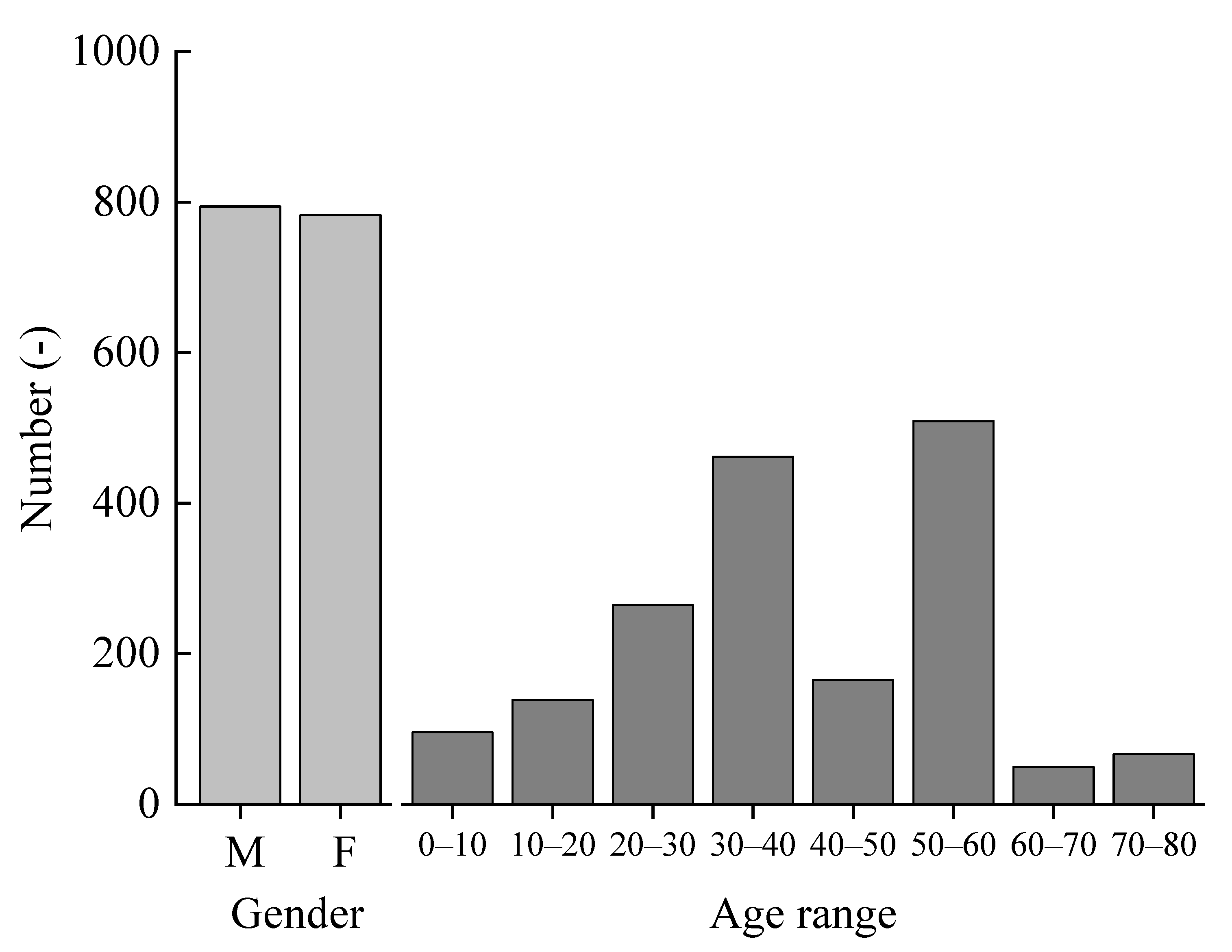
The results obtained from this survey were tabulated. A total of 1577 votes were obtained. Figure 3 shows the distribution of occupants by gender and age. The total number of votes obtained in this survey was 794 for male and 783 for female. The age distribution of the surveyed population was dominated by those in their 50s, followed by those in their 30s.

Table 5. Statistical summary of thermal environment data and thermal comfort indices.

	Unit	Mean	S.D.	Median
Indoor air temperature	°C	29.1	2.0	29
Indoor relative humidity	%	63.2	10.2	63
Indoor air velocity	m/s	0.1	0.0	0.1
Globe temperature	°C	28.9	1.9	28.9
Wet-bulb temperature	°C	23.5	2.5	24.1
Dew point temperature	°C	21.1	3.4	21.9
Foot temperature	°C	28.4	2.0	28.4
Outdoor air temperature	°C	28.8	2.5	28.5
Outdoor relative humidity	%	69.7	12	70
Outdoor air velocity	m/s	2.4	1.3	2.1
Atmospheric pressure	hPa	1012.6	4.1	1012
Cloud cover	–	6.7	2.5	6
Operative temperature	°C	29	1.9	29
Neutral temperature	°C	27.2	2.4	27.1
WBGT	°C	25.1	2.2	25.6
ET *	°C	29.2	2.0	29.3
SET *	°C	25.1	3.4	24.7
MRT	°C	28.9	1.9	28.9
30-WBGT	°C	4.9	2.2	4.4
Tdiff	°C	1.9	2.5	1.9
Metabolic rate	met	1.3	0.4	1.0
Clothing insulation	clo	0.43	0.2	0.39

WBGT: wet bulb globe temperature; ET *: new effective temperature; SET *: standard new effective temperature; MRT: mean radiant temperature; 30-WBGT: difference between WBGT-30 °C and current WBGT; Tdiff: difference between operative temperature and neutral temperature.

shows a statistical summary of the thermal environment data and thermal comfort indices. The minimum and maximum indoor air temperatures were 24.0 °C and 36.3 °C, respectively, with an average value of 29.1 °C. The minimum, maximum, and average indoor relative humidity were 35.1%, 91.0%, and 63.2%, respectively. The indoor thermal environment was close to that of a typical Japanese house in summer. The minimum, maximum, and mean outdoor air temperatures were 24.4 °C, 36.5 °C, and 28.8 °C, respectively. The minimum, maximum, and mean outdoor relative humidity were 38%, 91%, and 69.7%, respectively. The outdoor thermal environment was equivalent to the general climate of Gifu in summer.

Figure 4 depicts the indoor thermal-environment conditions. The natural ventilation state is indicated by NV, the cooling operation state is indicated by AC, and the state without natural ventilation and cooling is indicated by FR. NV and AC were approximately 35% and 50%, respectively, whereas NV + AC was only 2.9%. Figure 4 demonstrates that few people use natural ventilation and cooling simultaneously, suggesting a trade-off relationship.

Table 6. Statistical summary of subjective votes.

	Proportion (%)
Thermal sensation	Cool	Neutral	Warm
	2.1	68.7	29.2
Thermal conscious	Unconscious		Conscious
	47.6		52.4
Thermal acceptability	Unacceptable		Acceptable
	14.4		85.6
Thermal tolerance	Intolerable		Tolerable
	12.4		87.6
Affective assessment	Uncomfortable		Comfortable
	23.0		77.0
Thermal preference	Cooler	No change	Warmer
	56.0	42.5	1.5

The number of all subjective votes was 1577.

provides a statistical summary of subjective vote. In tabulating the data, reclassification was performed in terms of thermal sensation and affective assessment. For thermal sensation, “very cold”, “cold”, and “cool”, which had scale values ranging from −4 to −2, were considered to be cold; “slightly cool”, “neither hot nor cold”, and “slightly warm”, which had scale values ranging from −1 to +1, were considered to be neutral; and “warm”, “hot”, and “very hot”, which had scale values ranging from +2 to +4, were considered to be hot. For affective assessment, “extremely uncomfortable”, “very uncomfortable”, and “uncomfortable”, which had scale values ranging from +1 to +3, were considered to be uncomfortable, whereas “somewhat uncomfortable” and “comfortable”, which had scale values ranging from +4 to +5, were considered to be comfortable.

3.2. Analysis Using All Variables

To analyze the factors affecting natural ventilation in summer, we employed 10 machine learning models with window opening/closing as the objective variable and the characteristics obtained from the thermal environment survey and subjective report survey as explanatory variables. The features used in the analysis are shown in

Table 7. Features used in the analysis.

		Features
Thermal environmental data	Indoor	Indoor air temperature, indoor relative humidity, indoor air velocity, globe temperature, wet bulb temperature, dew-point temperature, foot temperature
	Outdoor	Outdoor air temperature, outdoor relative humidity, outdoor air velocity, atmospheric pressure, cloud cover
Thermal comfort indices		Operative temperature, neutral temperature, WBGT, ET *, SET *, MRT, 30-WBGT, Tdiff
Subjective vote		Thermal sensation, thermal conscious, thermal acceptability, thermal tolerance, Affective assessment, thermal preference
Human factor		Gender, age, metabolic rate, clothing insulation
Adaptation		Cooling, fan
Other		Date/time

.

Table 8. Comparison of machine learning models using all features.

Model	Accuracy (%)	Precision (%)	Recall (%)	F-Measure (%)
NB	72.6	57.9	83.8	68.5
LR	81.2	67.9	88.9	77.0
DT	80.3	66.0	91.8	76.7
RF	81.3	67.0	93.2	77.9
GBDT	84.3	73.9	86.5	79.7
GPR	79.1	66.0	84.0	74.0
SVM	69.4	65.8	27.7	38.9
MLP	83.9	72.9	87.3	79.4
NN	84.7	76.6	86.0	81.1
DNN	84.6	73.9	88.0	80.3

compares the machine learning models from an analysis using all variables. The accuracy was the highest for the NN approach at 84.7%. The machine learning model with the lowest accuracy was NB, at 72.6%. The NN approach also had the highest precision and F-measure values among the considered machine learning models. The recall for SVM was extremely low compared to those of the other models.

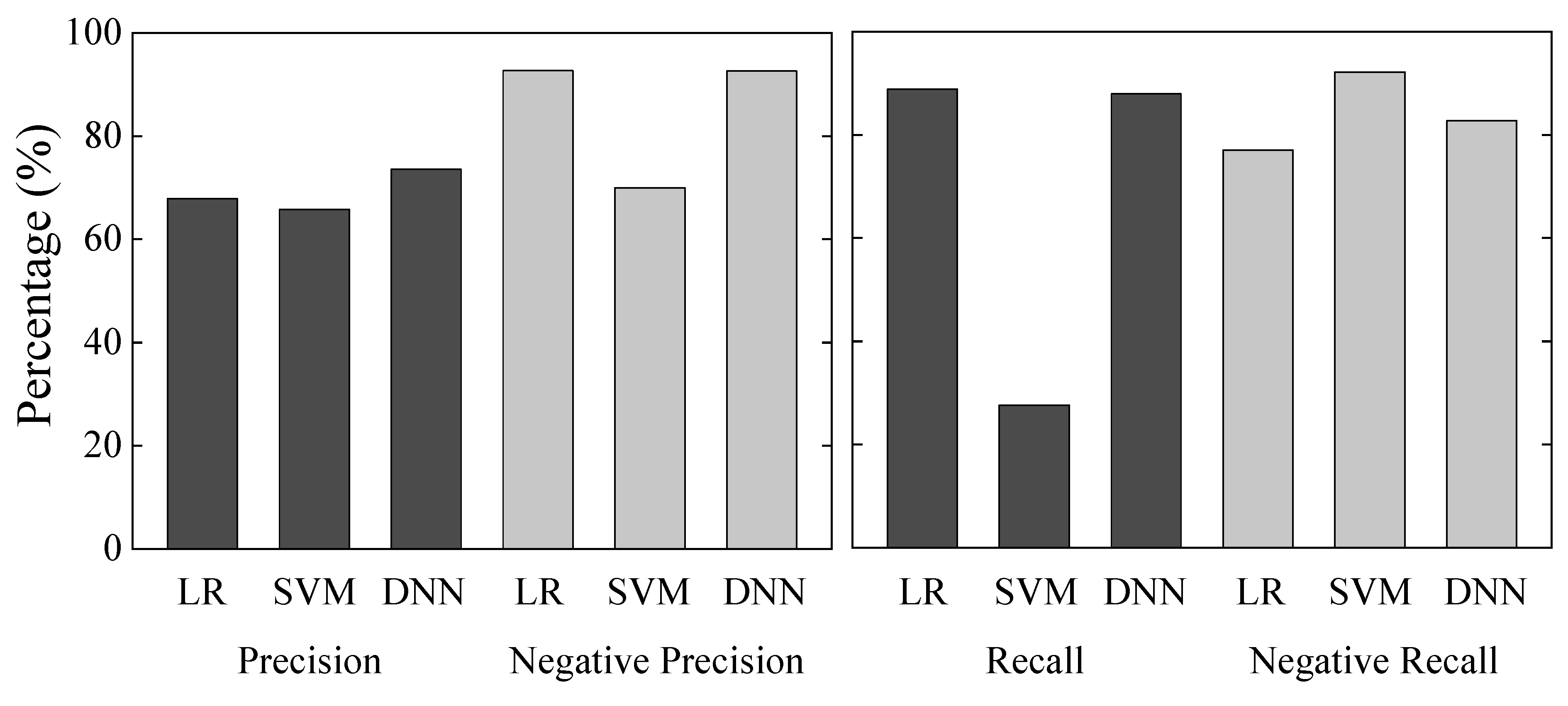
In order to analyze window-opening and -closing predictions in more detail, we divided the analysis into predictions for open windows and predictions for closed windows. Three models from the 10 machine learning models were representative. The three models used as representatives were LR, SVM, and DNN, which are widely used in previous studies. LR without hidden layers and DNN with hidden layers were selected as models with good accuracy, and SVM was selected as a model with poor accuracy. Figure 5 compares Precision, Negative Precision, Recall, and Negative Recall. Precision is the percentage of votes for which the window was actually open, among the votes for which the window was predicted to be open in the machine learning model. Negative Precision is the percentage of votes in which the window was actually closed, among the votes in which the window was predicted to be closed. Recall represents the percentage of votes that could be predicted to have an open window, among the votes that actually have an open window. Negative Recall represents the percentage of votes for which the window could be predicted to be closed, among the votes for which the window was actually closed. Precision was the highest for the DNN approach, at 73.9%, whereas those for the LR and SVM methods were 67.9% and 65.8%, respectively, with no significant differences compared to those of the other models. Negative Precision was comparable for the LR and DNN methods at 92.7% and 92.6%, respectively, whereas that of the SVM approach was lower than those of the other models, at 70.0%. Recall was 88.9% for the LR model and 88.0% for the DNN approach, whereas that of the SVM method was significantly lower, at 27.7%. Negative Recall was 77.1% for the LR method, 92.2% for the SVM approach, and 82.7% for the DNN technique, with the SVM model having the highest rate. This finding suggests that the LR and DNN approaches make correct predictions in terms of both window openings and window closings, but the SVM method is biased in its predictions. As the purpose of the SVM model is to draw a margin-maximizing boundary, it may not be suitable for analyses with a large number of features.

3.3. Analysis Using Feature Selection

In machine learning, a large number of features is important; however, interactions may lead to poor prediction accuracy. Therefore, it is important to perform feature selection to improve prediction accuracy. Feature selection leads to a shorter training time, simpler model interpretation, improved model accuracy, and reduced over-fitting. There are three major types of feature selection methods: the filter, wrapper, and embedded methods. The filter method does not use a machine learning model but rather is complete with only a data set. Thus, it has the advantage of a low computational cost as it depends on the performance of the data. On the other hand, the disadvantage is that only one feature is seen at a time, so the interaction of multiple features is not taken into account. The wrapper method uses multiple features simultaneously to verify prediction accuracy, searching for the combination with the highest accuracy. It is possible to find relationships between features that are not found with the filter method and to find the optimal combination of features for each model. In the embedded method, feature selection is performed during model training. In this study, feature selection was conducted using backward elimination, which is a wrapper method. The reason for using the wrapper method in this study is that provides more accurate feature selection than the other methods, even though it is computationally more expensive. Backward elimination was performed on each machine learning model to find the optimal combination of features.

Table 9. Features selected for backward elimination.

Feature	NB	LR	DT	RF	GBDT	GPR	SVM	MLP	NN	DNN
Indoor air temperature	●		●		●	●				●
Indoor relative humidity	●					●	●		●	●
Indoor air velocity					●				●	●
Globe temperature			●		●		●		●	●
Wet-bulb temperature							●	●	●	●
Dew point temperature		●					●		●	●
Foot temperature					●		●	●	●	●
Outdoor air temperature		●	●				●			●
Outdoor relative humidity		●				●			●	●
Outdoor air velocity	●					●				●
Atmospheric pressure			●		●		●		●
Cloud cover	●						●		●	●
Operative temperature					●		●	●	●	●
Neutral temperature					●		●		●	●
WBGT						●	●			●
ET *			●		●		●			●
SET *					●		●	●	●	●
MRT			●						●
30-WBGT			●				●		●
Tdiff		●	●		●		●		●	●
Thermal sensation		●					●			●
Thermal conscious	●		●				●	●	●	●
Thermal acceptability		●			●	●	●	●	●	●
Thermal tolerance		●	●			●	●	●	●	●
Affective assessment							●		●
Thermal preference	●	●	●		●	●	●			●
Gender	●	●	●	●	●	●	●	●	●	●
Age						●	●	●	●	●
Metabolic rate		●	●		●	●	●		●	●
Clothing insulation	●		●			●	●		●	●
Cooling	●	●	●	●	●	●	●	●	●	●
Fan	●	●				●	●	●	●	●
Date/time	●		●		●	●	●	●	●

shows the features chosen for backward elimination. The block circles show the features selected for each machine learning model. Although the selected optimal features varied with the model, the cooling feature was chosen for all the models, which implied that the influence of the cooling variable on the window opening/closing behavior was stronger than those of the other variables. Similarly, the gender feature was selected in all machine learning models, considering the possibility that the gender feature value poses a stronger influence on the occupant behavior for natural ventilation than other features.

Table 10. Comparison of machine learning models with analysis using feature selection.

Model	Accuracy (%)	Precision (%)	Recall (%)	F-Measure (%)
NB	81.0	67.5	89.8	77.0
LR	81.7	68.4	90.1	77.8
DT	81.9	68.5	90.9	78.1
RF	84.4	71.5	93.0	80.9
GBDT	84.5	73.0	89.4	80.4
GPR	82.8	71.2	87.1	78.3
SVM	80.7	66.6	91.7	77.2
MLP	86.8	76.6	90.6	83.1
NN	87.0	78.1	88.3	82.9
DNN	85.2	73.8	90.8	81.4

compares the machine learning models based on analysis using feature selection. Feature selection improved the accuracy of the analysis with all variables for all machine learning models. The model with the highest accuracy was the NN approach, at 87.0%, and the model with the lowest accuracy was the SVM method, at 80.7%. There were no particularly low values of precision, recall, or F-measure. Feature selection enabled all machine learning models to show high prediction accuracy.

Figure 6 compares Precision, Negative Precision, Recall, and Negative Recall in this section. The Precision was the highest for the DNN approach, at 73.8%. The LR and SVM models had Precision of 68.4% and 66.6%, respectively, with no significant differences among the machine learning models. Negative Precision was the highest for the SVM approach, at 94.3%. Negative Precision of the LR and DNN methods were 93.5% and 94.2%, respectively, which were high among the considered models. Recall was 90.1%, 91.7%, and 90.8%, and Negative Recall was 77.2%, 74.6%, and 82.1%, for the LR, SVM, and DNN approaches, respectively. While the results in Section 3.2 show differences among models, the results in Section 3.3 show little difference among models. By selecting features that were considered optimal for each model, it was possible to achieve high prediction accuracy through machine learning.

3.4. Analysis Using Thermal Indices of Room

In the previous section, machine learning was performed using all features. However, the more features there are, the more difficult it becomes to reflect them in a general study. Therefore, it was necessary to devise a mechanism to maintain the high accuracy of the machine learning models by utilizing a small number of features. As described in this section, machine learning was performed by setting the features and analyzing the variations in the evaluation indices. The indoor thermal environment has the potential to influence the window opening/closing behavior of the occupants significantly. In particular, globe temperature has been used as a thermal index representative of the indoor environment in previous studies [47]. In this study, we performed machine learning using globe temperature as a thermal index representative of indoor temperature.

Table 11. Comparison of machine learning models with globe temperature analysis.

Model	Accuracy (%)	Precision (%)	Recall (%)	F-Measure (%)
NB	67.5	53.3	67.3	59.5
LR	67.2	52.8	67.8	59.4
DT	56.1	44.8	91.6	60.2
RF	64.1	49.6	83.7	62.3
GBDT	60.9	47.1	88.0	61.4
GPR	64.9	50.3	79.0	61.4
SVM	65.9	51.3	73.6	60.5
MLP	64.4	50.1	80.3	61.7
NN	63.9	49.5	81.0	61.5
DNN	60.2	46.7	88.5	61.1

compares the machine learning models from the analysis with globe temperature. The prediction accuracy obtained by using globe temperature was lower than that resulting from using all variables and feature selection. The model with the highest accuracy was the NB approach, at 67.5%, and the model with the lowest accuracy was the DT method, at 56.1%. Compared to the analysis using feature selection, the accuracy was on average approximately 20% lower. Previous studies [18] have continuously investigated window conditions in naturally ventilated office buildings in the UK, with globe temperature as a feature affecting window conditions. Although this study intermittently investigated window conditions, it showed that globe temperature alone is only 50% to 60% accurate in predicting window opening and closing.

Figure 7 compares Precision, Negative Precision, Recall, and Negative Recall in this section. Precision was 52.8%, 51.3%, and 46.7%, and Negative Precision was 79.2%, 81.1%, and 87.7%, for the LR, SVM, and DNN approaches, respectively. In the analysis based on globe temperature, the prediction accuracy for actual window openings was approximately 50% for all machine learning models, but the prediction accuracy for window closings was approximately 80%, showing a large difference in prediction accuracy between window openings and closings. Recall was 67.8%, 73.6%, and 88.5%, and Negative Recall was 66.8%, 61.8%, and 44.7%, for the LR, SVM, and DNN models, respectively. The LR approach had similar prediction accuracy for Recall and Negative Recall, and the DNN approach showed a large difference in prediction accuracy between Recall and Negative Recall.

3.5. Analysis Using Experiential Temperature Thermal Factors

In the previous section, only globe temperature was used in the machine learning analysis. On the other hand, there are other characteristics that constitute the indoor environment besides globe temperature. The six components of the indoor thermal environment are air temperature, humidity, airflow, radiation, metabolic rate, and clothing insulation. Air temperature, humidity, airflow, and radiation are the four environmental factors, whereas metabolic rate and clothing insulation are the two human-body factors. However, no studies have used these thermal factors simultaneously in predicting window conditions. This section presents an analysis of the extent to which these thermal factors that constitute the perceived temperature affect occupant behavior with natural ventilation.

Table 12. Comparison of machine learning models based on analysis with six indoor thermal factors.

Model	Accuracy (%)	Precision (%)	Recall (%)	F-Measure (%)
NB	68.7	54.7	72.2	62.2
LR	69.0	54.3	77.0	63.7
DT	60.2	46.9	89.4	61.5
RF	66.1	51.2	88.9	65.0
GBDT	69.4	54.2	89.0	67.4
GPR	72.3	57.6	82.2	67.8
SVM	65.7	53.3	23.5	32.6
MLP	69.8	55.4	82.0	66.1
NN	70.3	55.5	82.8	66.4
DNN	63.9	49.6	90.3	64.0

compares machine learning models based on an analysis using six indoor thermal factors. The accuracy obtained from the analysis using the six indoor temperature factors was lower than the analysis using all variables and variable selection but higher than the analysis using globe temperature. The model with the highest accuracy was the GPR approach at 72.3%, and the model with the lowest accuracy was DT at 60.2%. DT, RF, GBDT, and DNN had Recall values close to 90%. Of these, DT, RF, and GBDT are tree-type machine learning models. Therefore, the analysis by the six indoor thermal factors showed that a tree-type model has a higher recall. In addition, the SVM recall was significantly lower than those of the other models, at 23.5%. The SVM method shows large differences in recall values depending on the features used for machine learning.

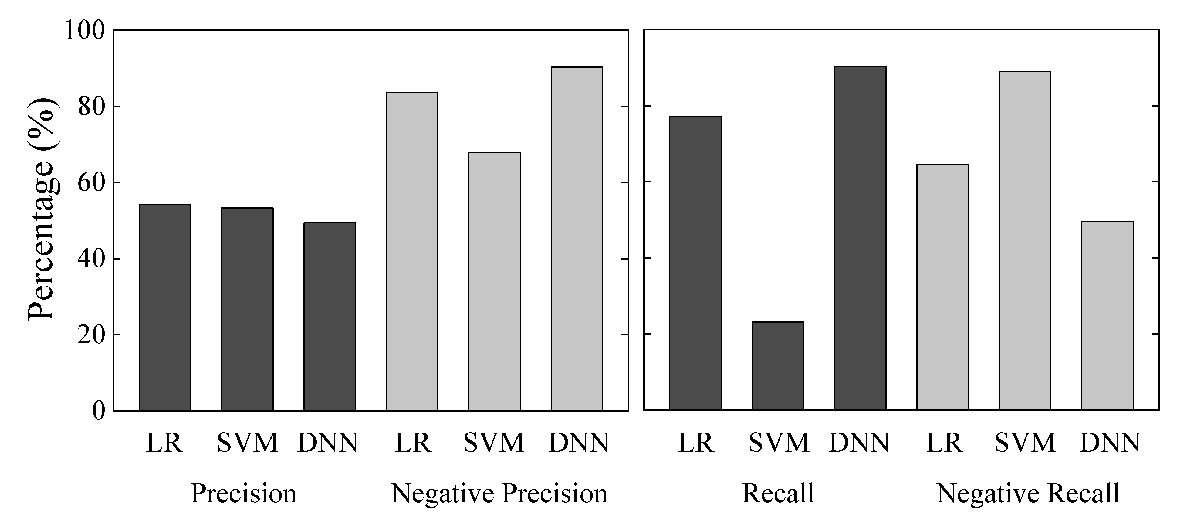
Figure 8 compares Precision, Negative Precision, Recall, and Negative Recall presented in this section. Precision was 54.3%, 53.3%, and 49.6%, and Negative Precision was 83.7%, 67.9%, and 90.3%, for the LR, SVM, and DNN models, respectively. Compared to the results in Section 3.4, in which only globe temperature was used as a feature, Precision had a slightly better prediction accuracy in all models. On the other hand, Negative Precision showed that the LR and DNN approaches yielded improved prediction accuracy, whereas the SVM technique decreased the prediction accuracy by 13.2%. These findings suggest that the LR and DNN approaches are effective for prediction using many features, whereas the SVM model is effective for prediction using few features. Recall was 77.0%, 23.5%, and 90.3%, and Negative Recall was 64.6%, 88.9%, and 49.5%, for the LR, SVM, and DNN models, respectively. Recall for SVM was extremely low. On the other hand, Negative Recall was as high as 88.9%, suggesting that the machine learning predictive votes were biased toward window closing.

3.6. Analysis Using Outdoor Thermal Indices

The previous section was machine learning by indoor thermal factors. On the other hand, the condition of the windows may be influenced by outdoor factors as well as indoor factors. Therefore, this section analyzes how outdoor air temperature affects window conditions. Outdoor thermal indicators are superior to indoor thermal indicators in that it is easier to obtain corresponding data. Therefore, a more efficient predictive model of window opening/closing behavior can be obtained if the accuracy of the analysis conducted using the outdoor thermal index is higher. In this section, machine learning is performed using the outdoor air temperature as a thermal index representative of the outdoors.

Table 13. Comparison of results of machine learning models for analysis based on outdoor air temperature.

Model	Accuracy (%)	Precision (%)	Recall (%)	F-Measure (%)
NB	55.4	35.4	32.2	33.7
LR	49.0	34.4	49.5	40.6
DT	58.0	34.4	20.9	26.0
RF	58.6	38.6	30.0	33.8
GBDT	42.4	36.7	87.4	51.7
GPR	55.3	37.4	38.1	37.7
SVM	48.2	33.5	49.8	40.1
MLP	49.1	34.9	51.3	41.5
NN	51.1	34.6	43.4	38.5
DNN	35.9	35.5	99.5	52.3

compares the machine learning models based on analysis using the outdoor air temperatures. The accuracy obtained in this manner was lower than that resulting from using a thermal index representative of the indoor air temperature. The model with the highest accuracy was the RF model, at 58.6%, and that with the lowest accuracy was the DNN approach, at 35.9%. Many of the models had low prediction accuracies, indicating that window-opening/closing behavior is not suitable for prediction with only outdoor-air-temperature features.

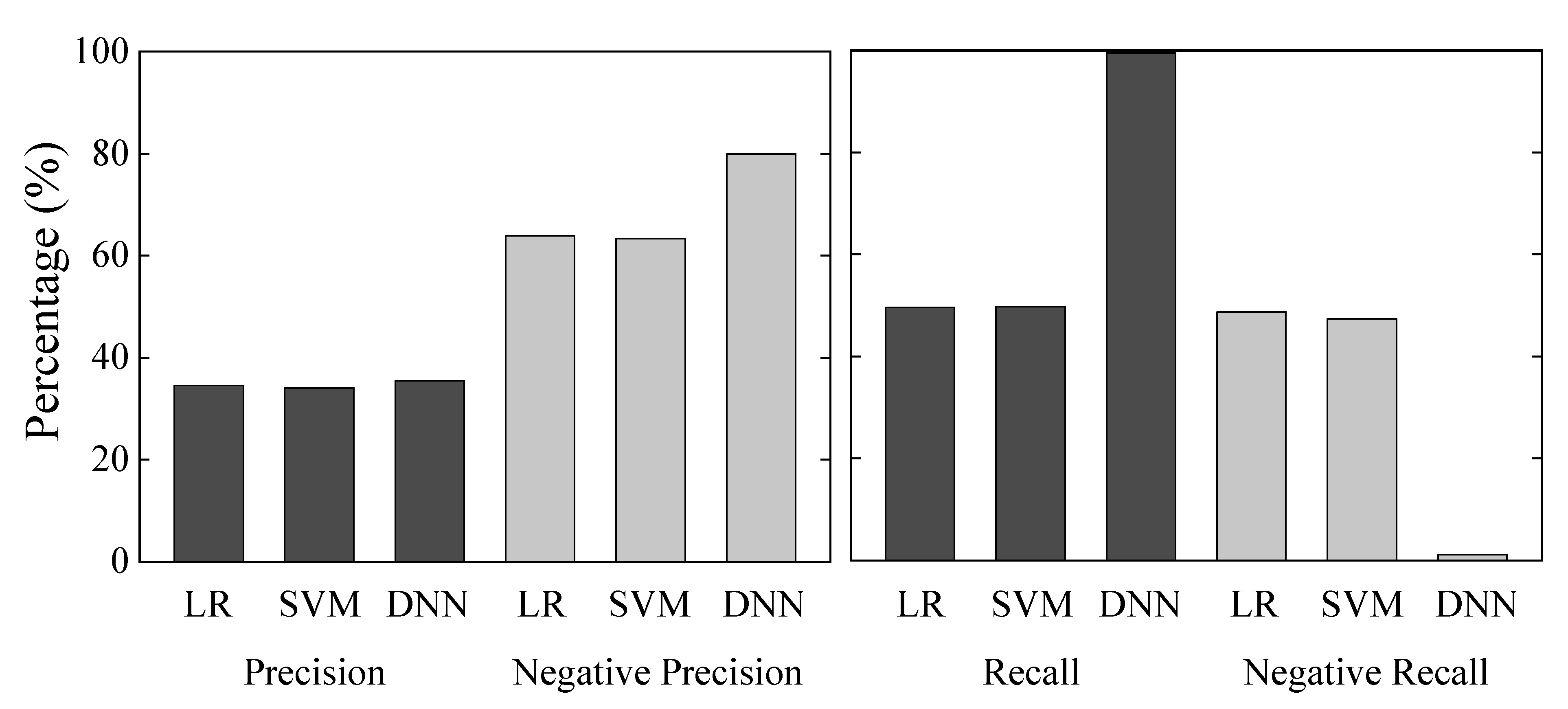
Figure 9 compares Precision, Negative Precision, Recall, and Negative Recall presented in this section. Precision was 34.4%, 33.5%, and 35.5%, and Negative Precision was 63.9%, 63.3%, and 80.0%, for the LR, SVM, and DNN models, respectively. Negative Precision for the DNN was higher than those of the other models but lower than those presented in the previous sections. Precision was also low, at approximately 35%, for all models. Recall was 49.5%, 49.8%, and 99.5%, and Negative Recall was 48.7%, 47.4%, and 1.2%, for the LR, SVM, and DNN models, respectively. For Recall and Negative Recall, the results were characterized by the DNN approach, with a large window bias in forecast votes. For predictions based on a single feature that changes little, such as outdoor air temperature in summer, the DNN approach is not considered particularly suitable compared to the other models.

3.7. Analysis Using Outdoor Environment Thermal Factors

In the previous section, machine learning was performed using only outdoor air temperature to predict window conditions. On the other hand, there are other factors besides air temperature that make up the outdoor environment. The use of outdoor thermal factors in the features may provide an improvement in accuracy. The analysis presented in this section was conducted using the outdoor relative humidity, outdoor air velocity, atmospheric pressure, and cloud cover, in addition to the outdoor air temperature, as the thermal factors that constitute the outdoor environment. We investigated the degree to which the prediction accuracy could be improved compared to when the outdoor air temperature alone was used.

Table 14. Comparison of results of machine learning models based on analysis of outdoor thermal factors.

Model	Accuracy (%)	Precision (%)	Recall (%)	F-Measure (%)
NB	58.1	42.9	57.5	49.1
LR	62.2	47.4	58.2	52.2
DT	61.0	47.7	44.5	46.0
RF	56.7	43.2	64.5	51.8
GBDT	58.9	45.9	85.8	59.8
GPR	62.4	47.8	65.2	55.2
SVM	60.3	45.4	58.2	51.0
MLP	61.4	47.2	62.3	53.7
NN	60.9	46.6	61.9	53.2
DNN	46.7	39.7	90.3	55.2

compares the machine learning models based on analysis using outdoor thermal factors. The prediction accuracy obtained from the analysis using the outdoor thermal factor was higher than that resulting from using only the outdoor air temperature. The model with the highest accuracy was the GP model, at 62.4%, and the lowest was the DL approach, at 46.7%. Compared to the analysis using only outdoor air temperature, using the outdoor thermal factors improved the accuracy by an average of 8.6%. Therefore, the outdoor relative humidity, outdoor air velocity, atmospheric pressure, and cloud cover may affect indoor human behavior only slightly. On the other hand, the analysis using the outdoor thermal factor resulted in a 4.7% lower mean accuracy compared to that obtained using only globe temperature. These results suggest that the window-opening and -closing behaviors of occupants are more strongly influenced by indoor thermal factors than outdoor factors.

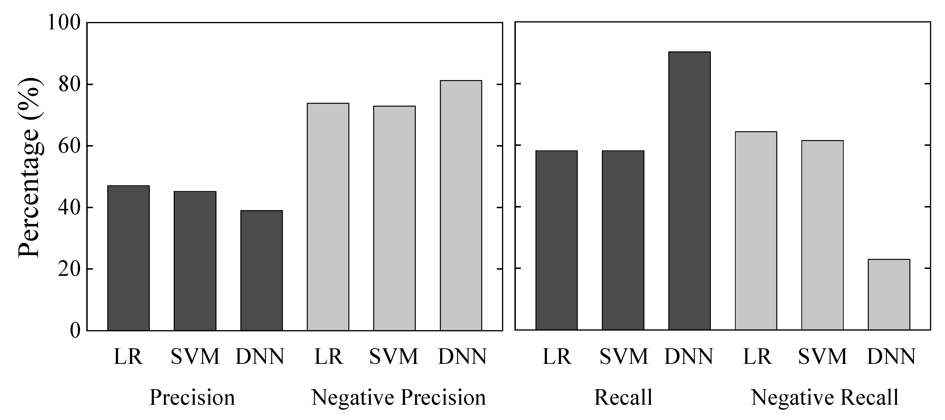
Figure 10 compares Precision, Negative Precision, Recall, and Negative Recall presented in this section. Precision was 47.4%, 45.4%, and 39.7%, and Negative Precision was 73.8%, 72.9%, and 81.3%, for the LR, SVM, and DNN methods, respectively. Both Precision and Negative Precision were improved compared to those presented in Section 3.6. Both the LR and SVM results were improved by approximately 10% compared to those in Section 3.6, whereas the DNN results were improved by only approximately 1%. Recall was 58.2%, 58.2%, and 90.3%, and Negative Recall was 64.3%, 61.5%, and 22.9%, for the LR, SVM, and DNN models, respectively. Similar to the results in Section 3.6, the DNN was biased in its predictive votes. However, Negative Recall was improved by approximately 20%, suggesting that the situation improved slightly.

3.8. Analysis Using Thermal Indices Representative of Indoor and Outdoor Environments

In the previous section, machine learning was used with outdoor environmental factors to predict window conditions. Outdoor environmental factors did not provide sufficient accuracy in predicting window conditions. Therefore, we will examine whether useful accuracy can be obtained by using indoor and outdoor factors. The analysis was conducted using globe temperature as a thermal index representative of the indoor area and the outdoor air temperature as a thermal index representative of the outdoor area.

Table 15. Comparison of results of machine learning models based on analysis with globe and outdoor air temperatures.

Model	Accuracy (%)	Precision (%)	Recall (%)	F-Measure (%)
NB	67.0	52.5	65.3	58.2
LR	68.7	54.2	77.0	63.6
DT	54.9	43.8	93.5	59.6
RF	61.9	47.9	87.3	61.8
GBDT	63.3	49.0	86.2	62.5
GPR	68.2	53.2	84.0	65.2
SVM	67.3	52.5	85.6	65.1
MLP	68.2	53.4	83.8	65.3
NN	66.5	51.6	86.2	64.6
DNN	64.1	49.7	85.8	62.9

compares the machine learning models based on analysis using globe temperature and outdoor air temperature. The model with the highest accuracy was the LR model, at 68.7%, and the lowest was the DT approach, at 54.9%. The analysis using both globe temperature and outdoor air temperature was more accurate than that using globe temperature or outdoor air temperature alone. On the other hand, the accuracy in this section was approximately 1.5% better than that obtained using only globe temperature. Therefore, globe temperature and outdoor air temperature alone are not considered sufficient features for predicting window-opening and -closing behavior.

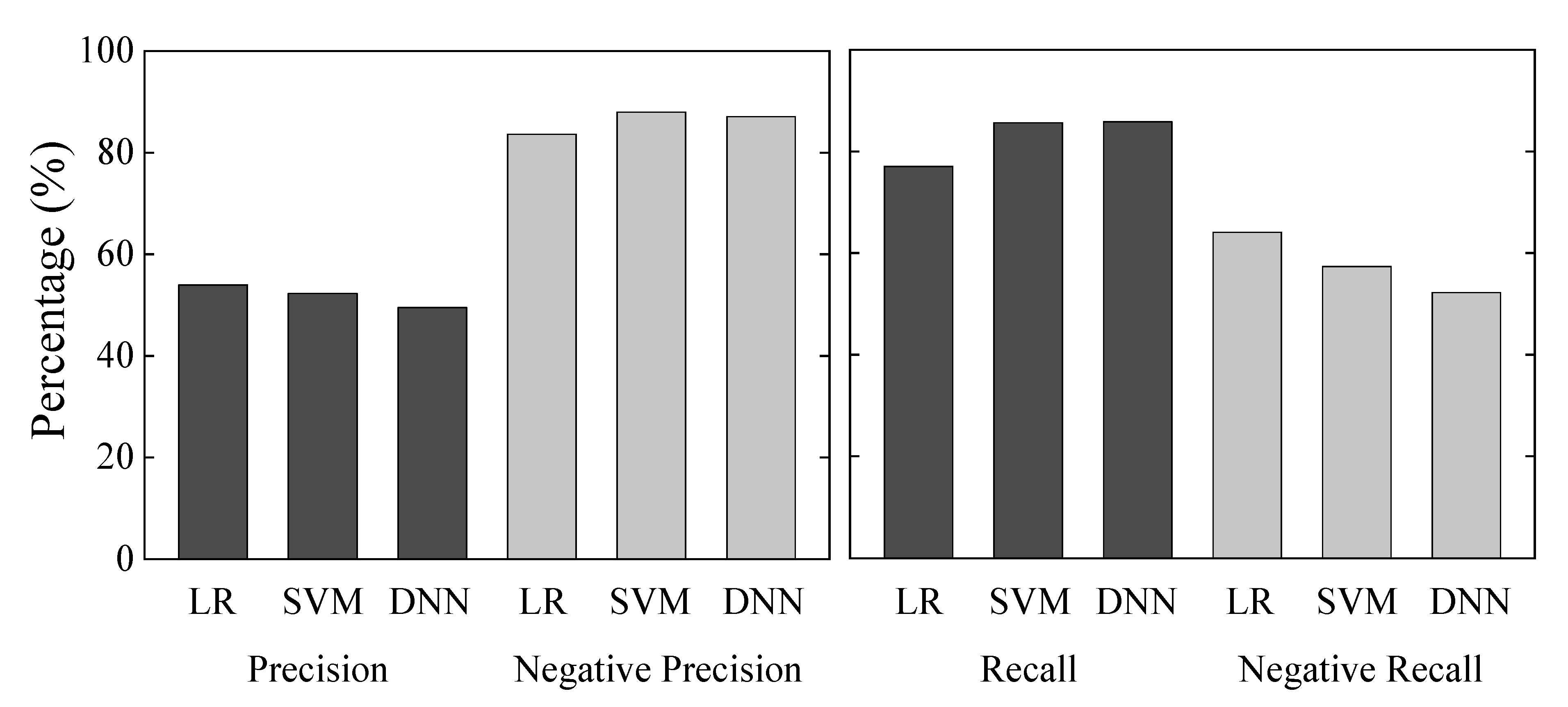
Figure 11 compares Precision, Negative Precision, Recall, and Negative Recall presented in this section. Precision was 54.2%, 52.5%, and 49.7%,, and Negative Precision was 83.6%, 88.0%, and 87.1%, for the LR, SVM, and DNN models, respectively. There was not much difference in Precision or Negative Precision between the different models. Recall was 77.0%, 85.6%, and 85.8%, and Negative Recall was 64.1%, 57.4%, and 52.3%, for the LR, SVM, and DNN models, respectively. Recall and Negative Recall also did not differ much from those in the other sections due to differences between the models.

3.9. Analysis of Representative Indoor Thermal Indices and Cooling

Cooling is used in Japanese summer homes to avoid heat. When cooling is in use, people often close doors and windows in order to cool rooms efficiently, and previous studies have shown that there is a trade-off between cooling and window features [48]. In addition, the fact that the cooling feature was selected for all machine learning models in feature selection suggests that the influence of cooling plays a significant role in window-opening and -closing behavior. Although it has been shown that there is a trade-off relationship between these factors, no study has been conducted using the features of cooling to predict window-opening and -closing behavior, and it has not been shown to what extent the features of cooling improve the prediction of window-opening and -closing behavior. Cooling usage data has become easier to acquire automatically in recent years due to the development of the Internet of Things (IoT). If features that have a trade-off relationship can be shown to be effective in predicting natural ventilation behavior, the results will be significant from an engineering use perspective. Therefore, in this section, machine learning was performed by adding cooling features to globe temperature, and an analysis was conducted to determine by how much the prediction accuracy could be improved.

Table 16. Comparison of results of machine learning models based on analysis considering globe temperature and cooling.

Model	Accuracy (%)	Precision (%)	Recall (%)	F-Measure (%)
NB	80.5	66.2	91.8	76.9
LR	80.3	66.0	91.8	76.8
DT	80.1	66.0	90.5	76.3
RF	79.8	65.4	91.2	76.2
GBDT	79.8	65.3	91.9	76.4
GPR	80.2	65.9	91.6	76.6
SVM	80.3	66.0	91.8	76.8
MLP	80.3	65.9	91.8	76.7
NN	80.3	66.0	91.8	76.8
DNN	80.0	65.6	91.6	76.5

compares the machine learning models according to the analysis with globe temperature and cooling. The analysis using both globe temperature and cooling was between 13% and 24% more accurate than that performed using globe temperature alone, and it was as accurate as that conducted using all variables. The model with the highest accuracy was the NB model, at 80.5%, and the lowest was the RF approach, at 79.8%. The differences in prediction accuracy between the different models were smaller than those in the other sections.

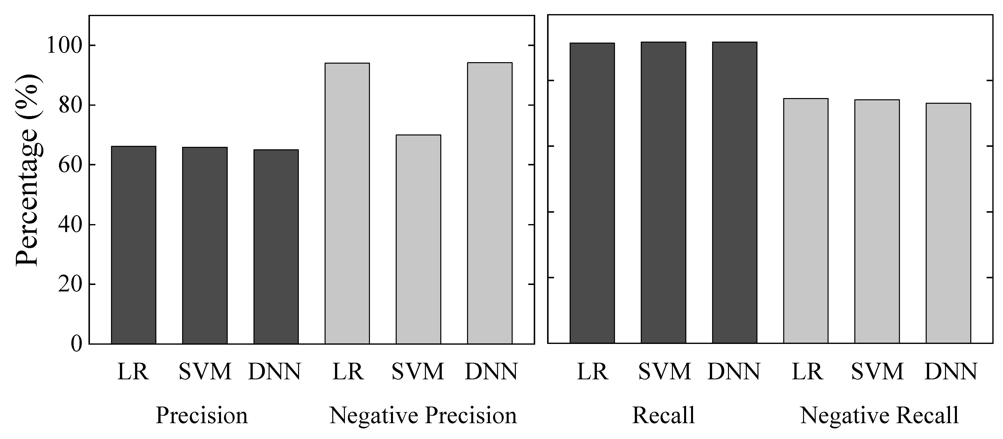
Figure 12 compares Precision, Negative Precision, Recall, and Negative Recall presented in this section. Precision was 66.0%, 66.0%, and 65.6%, and Negative Precision was 94.1%, 69.9%, and 94.2%, for the LR, SVM, and DNN models, respectively. Precision was similar for all models, whereas Negative Precision was higher for the LR and DNN approaches, at approximately 94%. Recall was 91.8%, 91.8%, and 91.6%, and Negative Recall was 74.5%, 74.1%, and 73.0%, for the LR, SVM, and DNN models, respectively. Recall and Negative Recall were close using any machine learning model. The trade-off between cooling features and windows suggests that cooling features may have a greater impact on window predictions than other features.

3.10. Investigation of Optimal Features Describing Window-Opening/Closing Behavior

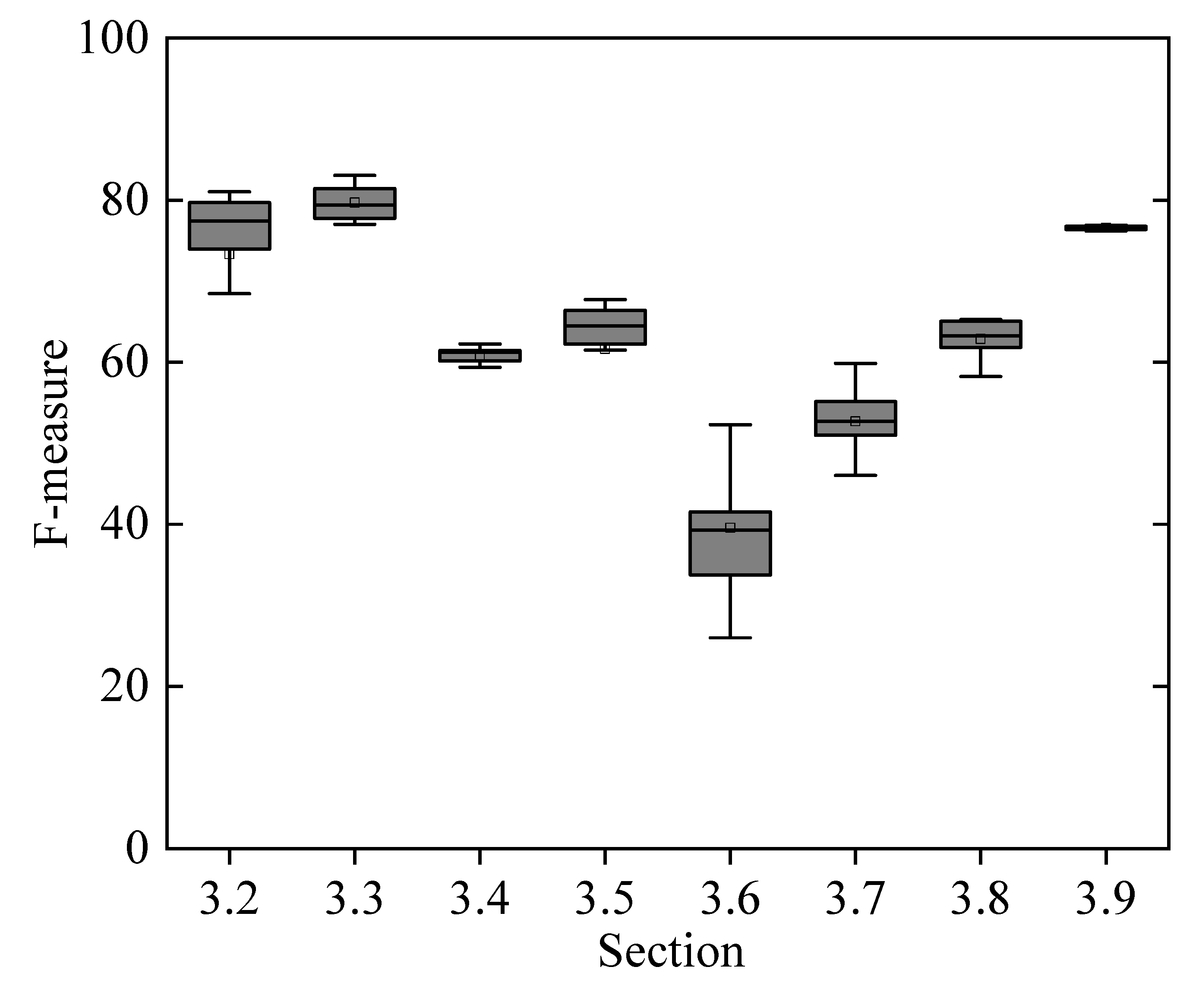
This section examines the extent to which accuracy is affected by the different features that have been used in Section 3.2, Section 3.3, Section 3.4, Section 3.5, Section 3.6, Section 3.7, Section 3.8 and Section 3.9. Figure 13 shows a comparison of the F-measure for the different features used. In Section 3.2. with all features and in Section 3.3. with feature selection, the F-measure was high. On the other hand, the analysis performed with fewer features did not provide useful accuracy in predicting window conditions. The F-measure for the analysis of indoor thermal environmental factors ranged from about 61% to 67%, and for the analysis using outdoor environmental factors, it ranged from about 49% to 60%. In the analysis where the cooling feature was added to globe temperature, the F-measure was approximately 76–77% of the value, indicating a valid result for adding the feature. The results in Section 3.9 suggest that one of the most effective means of improving the accuracy of predicting occupant behavior in terms of natural ventilation in summer is to use cooling features, which have a trade-off relationship.

3.11. Comparison with Previous Studies

The responses of the machine learning models to data imbalance and overall accuracy were analyzed using the F-measure. Haldi et al. [49] assessed the effects of occupancy patterns, indoor temperature, and outdoor climate parameters on window-opening and -closing behavior and developed modeling methods such as the LR and Markov chain approaches. Rijal et al. [18] proposed a window opening prediction model using LR and data from a thermal comfort survey conducted in a UK office building. They used globe temperature and outdoor air temperature to predict window conditions. Markovic et al. [50] used machine learning to predict window-opening and -closing behavior in German office buildings. They were predicted using data collected at the E.ON Energy Research Center and performed using 24 thermal environment features. Figure 14 compares the F-measures obtained in these previous studies and in the present study. For all models (the LR, SVM, and DNN models), the maximum value of the F-measure exceeded the results of previous studies. Therefore, it is possible to improve the accuracy of window opening and closing by combining features. On the other hand, as this study did not include hyperparameters, further improvement in accuracy can be expected.

4. Conclusions

We used machine learning to analyze occupant behaviors in terms of natural ventilation in the summer in Japan. Ten machine learning models were compared, and the best model for predicting occupant behavior was considered. The best machine learning models differed depending on the features used, but, in general, the LR model without hidden layers and the DNN model with hidden layers showed superior accuracy. SVM showed lower accuracy than the other machine learning models. However, SVM also showed high accuracy depending on the features selected. Based on these results, it was not possible to select a single model that is best-suited for predicting window conditions. Another validity obtained in this study is that models such as LR, which do not have a hidden layer, showed accuracy close to that of DNNs with a hidden layer. Since LR can show predictions in regression equations, it would be possible for the simulation to reflect the occupants’ behavior schedule using the function equation.

In examining the features, the highest accuracy was obtained by performing feature selection using backward elimination for each individual model. With the COVID-19 pandemic, it will become increasingly important to have a clear picture of occupants’ natural-ventilation behavior. On the other hand, to increase the value of engineering applications, it is necessary to explore features for which data are easy to obtain in order to achieve high accuracy with a small number of features. Of the data used in this study, it is important to give priority to features that can be measured constantly, such as temperature and humidity. It is difficult to engineer features that require subjective votes or to develop other questionnaires to be used. Data regarding cooling features, which have a trade-off relationship with window opening/closing behavior, have become easier to obtain automatically in recent years with the development of the IoT. The analysis using globe temperature and cooling features showed higher accuracy than those using the other feature combinations. In the future, it will be important to predict window opening/closing behavior using features that can be measured at all times. However, this study was conducted only on houses in Gifu, Japan, with low airtightness and low thermal insulation. Future work is needed to analyze occupant behavior in homes in different climatic zones as well as in highly insulated homes.

References

1. Huovila, P.; Ala-Juusela, M.; Melchert, L.; Pouffary, S.; Cheng, C.C.; Ürge-Vorsatz, D.; Koeppel, S.; Svenningsen, N.; Graham, P. Buildings and Climate Change: Summary for Decision Makers; Sustainable United Nations; United Nations Environment Programme: Nairobi, Kenya, 2009. [Google Scholar]
2. Congedo, P.M.; Baglivo, C.; Seyhan, A.K.; Marchetti, R. Worldwide dynamic predictive analysis of building performance under long-term climate change conditions. J. Build. Eng. 2021, 42, 103057. [Google Scholar] [CrossRef]
3. Carlucci, S.; Causone, F.; Biandrate, S.; Ferrando, M.; Moazami, A.; Erba, S. On the impact of stochastic modeling of occupant behavior on the energy use of office buildings. Energy Build. 2021, 246, 111049. [Google Scholar] [CrossRef]
4. Du, J.; Pan, W. Diverse occupant behaviors and energy conservation opportunities for university student residences in Hong Kong. Build. Environ. 2021, 195, 107730. [Google Scholar] [CrossRef]
5. Clevenger, C.; Haymaker, J.; Jalili, M. Demonstrating the impact of the occupant on building performance. J. Comput. Civ. Eng. 2014, 28, 99–102. [Google Scholar] [CrossRef]
6. Ioannou, A.; Itard, L.C.M. Energy performance and comfort in residential buildings: Sensitivity for building parameters and occupancy. Energy Build. 2015, 92, 216–233. [Google Scholar] [CrossRef]
7. Sun, K.; Hong, T. A simulation approach to estimate energy savings potential of occupant behavior measures. Energy Build. 2017, 136, 43–62. [Google Scholar] [CrossRef]
8. Wang, L.; Greenberg, S. Window operation and impacts on building energy consumption. Energy Build. 2015, 92, 313–321. [Google Scholar] [CrossRef]
9. Rijal, H.B.; Humphreys, M.A.; Nicol, J.F. Development of a window opening algorithm based on adaptive thermal comfort to predict occupant behavior in Japanese dwellings. Jpn. Archit. Rev. 2018, 1, 310–321. [Google Scholar] [CrossRef]
10. Andersen, R.; Fabi, V.; Toftum, J.; Corgnati, S.P.; Olesen, B.W. Window opening behaviour modelled from measurements in Danish dwellings. Build. Environ. 2013, 69, 101–113. [Google Scholar] [CrossRef]
11. Shi, S.; Zhao, B. Occupants’ interactions with windows in 8 residential apartments in Beijing and Nanjing, China. Build. Simul. 2016, 9, 221–231. [Google Scholar] [CrossRef]
12. Jeong, B.; Jeong, J.-W.; Park, J.S. Occupant behavior regarding the manual control of windows in residential buildings. Energy Build. 2016, 127, 206–216. [Google Scholar] [CrossRef]
13. Jones, R.V.; Fuertes, A.; Gregori, E.; Giretti, A. Stochastic behavioural models of occupants’ main bedroom window operation for UK residential buildings. Build. Environ. 2017, 118, 144–158. [Google Scholar] [CrossRef]
14. Shi, S.; Li, H.; Ding, X.; Gao, X. Effects of household features on residential window opening behaviors: A multilevel logistic regression study. Build. Environ. 2020, 170, 106610. [Google Scholar] [CrossRef]
15. Fabi, V.; Andersen, R.K.; Corgnati, S. Verification of stochastic behavioural models of occupants’ interactions with windows in residential buildings. Build. Environ. 2015, 94, 371–383. [Google Scholar] [CrossRef]
16. Lai, D.; Jia, S.; Qi, Y.; Liu, J. Window-opening behavior in Chinese residential buildings across different climate zones. Build. Environ. 2018, 142, 234–243. [Google Scholar] [CrossRef]
17. Zhang, Y.; Barrett, P. Factors influencing the occupants’ window opening behaviour in a naturally ventilated office building. Build. Environ. 2012, 50, 125–134. [Google Scholar] [CrossRef]
18. Rijal, H.B.; Tuohy, P.; Humphreys, M.A.; Nicol, J.F.; Samuel, A.; Clarke, J. Using results from field surveys to predict the effect of open windows on thermal comfort and energy use in buildings. Energy Build. 2007, 39, 823–836. [Google Scholar] [CrossRef]
19. Herkel, S.; Knapp, U.; Pfafferott, J. Towards a model of user behaviour regarding the manual control of windows in office buildings. Build. Environ. 2008, 43, 588–600. [Google Scholar] [CrossRef]
20. Yun, G.Y.; Steemers, K. Time-dependent occupant behaviour models of window control in summer. Build. Environ. 2008, 43, 1471–1482. [Google Scholar] [CrossRef]
21. Haldi, F.; Robinson, D. On the behaviour and adaptation of office occupants. Build. Environ. 2008, 43, 2163–2177. [Google Scholar] [CrossRef]
22. Deme Belafi, Z.; Naspi, F.; Arnesano, M.; Reith, A.; Revel, G.M. Investigation on window opening and closing behavior in schools through measurements and surveys: A case study in Budapest. Build. Environ. 2018, 143, 523–531. [Google Scholar] [CrossRef]
23. Fathi, S.; Srinivasan, R.; Fenner, A.; Fathi, S. Machine learning applications in urban building energy performance forecasting: A systematic review. Renew. Sustain. Energy Rev. 2020, 133, 110287. [Google Scholar] [CrossRef]
24. Wang, Z.; Srinivasan, R. A review of artificial intelligence-based building energy use prediction: Contrasting the capabilities of single and ensemble prediction models. Renew. Sustain. Energy Rev. 2016, 75, 796–808. [Google Scholar] [CrossRef]
25. Tardioli, G.; Kerrigan, R.; Oates, M.; O’Donnell, J.; Finn, D. Data driven approaches for prediction of building energy consumption at urban level. Energy Procedia 2015, 78, 3378–3383. [Google Scholar] [CrossRef]
26. Wei, Y.; Zhang, X.; Shi, Y.; Xia, L.; Pan, S.; Wu, J.; Han, M.; Zhao, X. A review of data-driven approaches for prediction and classification of building energy consumption. Renew. Sustain. Energy Rev. 2018, 82, 1027–1047. [Google Scholar] [CrossRef]
27. Pham, A.-D.; Ngo, N.-T.; Ha Truong, T.T.; Huynh, N.-T.; Truong, N.-S. Predicting energy consumption in multiple buildings using machine learning for improving energy efficiency and sustainability. J. Clean. Prod. 2020, 260, 121082. [Google Scholar] [CrossRef]
28. Robinson, C.; Dilkina, B.; Hubbs, J.; Zhang, W.; Guhathakurta, S.; Brown, M.A.; Pendyala, R.M. Machine learning approaches for estimating commercial building energy consumption. Appl. Energy 2017, 208, 889–904. [Google Scholar] [CrossRef]
29. Li, K.; Xie, X.; Xue, W.; Dai, X.; Chen, X.; Yang, X. A hybrid teaching-learning artificial neural network for building electrical energy consumption prediction. Energy Build. 2018, 174, 323–334. [Google Scholar] [CrossRef]
30. Olu-Ajayi, R.; Alaka, H.; Sulaimon, I.; Sunmola, F.; Ajayi, S. Building energy consumption prediction for residential buildings using deep learning and other machine learning techniques. J. Build. Eng. 2022, 45, 103406. [Google Scholar] [CrossRef]
31. Kayoko, H. Thermal insulation of clothing. J. Textile Mach. Soc. Japan 1982, 35, P358–P364. [Google Scholar]
32. Japan Meteorological Agency. Available online: https://www.data.jma.go.jp/obd/stats/etrn/ (accessed on 27 June 2022).
33. American National Standards Institute; American Society of Heating, Refrigerating and Air-Conditioning Engineers. ANSI/ASHRAE Standard 55-2020: Thermal Environmental Conditions for Human Occupancy; American Society of Heating, Refrigerating and Air Conditioning Engineers, Inc.: Atlanta, GA, USA, 2020. [Google Scholar]
34. American Society of Heating, Refrigerating and Air Conditioning Engineers. ASHRAE Handbook—Fundamentals 2017 Chapter 9: Thermal Comfort; American Society of Heating, Refrigerating and Air Conditioning Engineers, Inc.: Atlanta, GA, USA, 2017. [Google Scholar]
35. RapidMiner|Amplify the Impact of Your People, Expertise & Data, RapidMiner. Available online: https://rapidminer.com/ (accessed on 27 June 2022).
36. Cheung, F.K.T.; Skitmore, M. Application of cross validation techniques for modelling construction costs during the very early design stage. Build. Environ. 2006, 41, 1973–1990. [Google Scholar] [CrossRef]
37. van Herwerden, D.; O’Brien, J.W.; Choi, P.M.; Thomas, K.V.; Schoenmakers, P.J.; Samanipour, S. Naive Bayes classification model for isotopologue detection in LC-HRMS data. Chemom. Intell. Lab. Syst. 2022, 223, 104515. [Google Scholar] [CrossRef]
38. Domingos, P. A few useful things to know about machine learning. Commun. ACM 2012, 55, 78–87. [Google Scholar] [CrossRef]
39. Wang, Z.; Wang, Y.; Zeng, R.; Srinivasan, R.S.; Ahrentzen, S. Random Forest based hourly building energy prediction. Energy Build. 2018, 171, 11–25. [Google Scholar] [CrossRef]
40. What Is the Difference between Bagging and Boosting? Quantdare, 2016. Available online: https://quantdare.com/what-is-the-difference-between-bagging-and-boosting/ (accessed on 27 June 2022).
41. Bienvenido-Huertas, D.; Rubio-Bellido, C.; Pérez-Ordóñez, J.L.; Moyano, J. Optimizing the evaluation of thermal transmittance with the thermometric method using multilayer perceptrons. Energy Build. 2019, 198, 395–411. [Google Scholar] [CrossRef]
42. Rasmussen, C.D. Gaussian processes in machine learning. In Revised Lectures; Bousquet, O., von Luxburg, U., Rätsch, G., Eds.; Springer: Berlin/Heidelberg, Germany, 2004; pp. 63–71. [Google Scholar]
43. Noble, W.S. What is a support vector machine? Nat. Biotechnol. 2006, 24, 1565–1567. [Google Scholar] [CrossRef]
44. Chan, S.Y.; Chau, C.K. Development of artificial neural network models for predicting thermal comfort evaluation in urban parks in summer and winter. Build. Environ. 2019, 164, 106364. [Google Scholar] [CrossRef]
45. Goodfellow, I.; Bengio, Y.; Courville, A. Deep Learning; MIT Press: Cambridge, MA, USA, 2016. [Google Scholar]
46. Payet, M.; David, M.; Lauret, P.; Amayri, M.; Ploix, S.; Garde, F. Modelling of occupant behaviour in non-residential mixed-mode buildings: The distinctive features of tropical climates. Energy Build. 2022, 259, 111895. [Google Scholar] [CrossRef]
47. Shrestha, M.; Rijal, H.B.; Kayo, G.; Shukuya, M. A field investigation on adaptive thermal comfort in school buildings in the temperate climatic region of Nepal. Build. Environ. 2021, 190, 107523. [Google Scholar] [CrossRef]
48. Psomas, T.; Fiorentini, M.; Kokogiannakis, G.; Heiselberg, P. Ventilative cooling through automated window opening control systems to address thermal discomfort risk during the summer period: Framework, simulation and parametric analysis. Energy Build. 2017, 153, 18–30. [Google Scholar] [CrossRef]
49. Haldi, F.; Robinson, D. Interactions with window openings by office occupants. Build. Environ. 2009, 44, 2378–2395. [Google Scholar] [CrossRef]
50. Markovic, R.; Grintal, E.; Wölki, D.; Frisch, J.; van Treeck, C. Window opening model using deep learning methods. Build. Environ. 2018, 145, 319–329. [Google Scholar] [CrossRef]
Figure 1. Trends in outdoor temperatures during the study period (August 2010).
Energies 15 05993 g001
Figure 2. Measurement instruments used.
Energies 15 05993 g002
Figure 3. Distribution of occupants by gender and age.
Energies 15 05993 g003
Figure 4. Indoor thermal environment conditions.
Energies 15 05993 g004
Figure 5. Comparison of Precision, Negative Precision, Recall, and Negative Recall in Section 3.2.
Energies 15 05993 g005
Figure 6. Comparison of Precision, Negative Precision, Recall, and Negative Recall in Section 3.3.
Energies 15 05993 g006
Figure 7. Comparison of Precision, Negative Precision, Recall, and Negative Recall in Section 3.4.
Energies 15 05993 g007
Figure 8. Comparison of Precision, Negative Precision, Recall, and Negative Recall in Section 3.5.
Energies 15 05993 g008
Figure 9. Comparison of Precision, Negative Precision, Recall, and Negative Recall in Section 3.6.
Energies 15 05993 g009
Figure 10. Comparison of Precision, Negative Precision, Recall, and Negative Recall in Section 3.7.
Energies 15 05993 g010
Figure 11. Comparison of Precision, Negative Precision, Recall, and Negative Recall in Section 3.8.
Energies 15 05993 g011
Figure 12. Comparison of Precision, Negative Precision, Recall, and Negative Recall in Section 3.9.
Energies 15 05993 g012
Figure 13. Comparison of F-measures presented in each section.
Energies 15 05993 g013
Figure 14. Comparison of F-measure between this study and previous studies.
Energies 15 05993 g014