1. Introduction
Significant efforts have been made worldwide in recent years to increase the penetration of renewable energy source (RES) use while improving building energy efficiency [
1]. Meanwhile, by increasing the penetration of intermittent RESs, it becomes increasingly important to develop and integrate technological solutions able to absorb RES-related disruptions and sustain power grid network operations [
2]. The reliable, uninterrupted operation of energy systems relies on the balance between the consumption and generation of energy in real-time, taking into account the variability of production (e.g., the weather-dependent part) and consumption (e.g., building demand profiles, consumer behaviour) [
3]. Therefore, the intelligent control of consumption patterns of buildings and/or districts becomes increasingly important due to its ability to mitigate electricity fluctuations and reduce the available grid power demands as well as the associated costs [
4].
The electricity sector in the European Union (EU) currently faces an unprecedented crossroads. The incumbent market’s key drivers comprise the existence of both short-term effective optimisation of existing production capacities and long-term investment prospects for the construction of new capacities. However, the high level of market distortion in the electricity sector has a negative impact on this function of the current market [
4]. In this regard, flexibility in Europe’s power systems is required to accommodate an increasing share of variable power generation from RESs. Indeed, service quality issues start to arise on the grid when this share in electricity consumption reaches 10%. To meet the EU’s targets for reduction in greenhouse gas (GHG) emissions, this share should rise to 30% by 2030 and up to 50% by 2050.
A possible solution to this challenge is the change from supply control to demand control, i.e., adapting the demand to the generated power. This change requires the increased use of advanced control and optimisation algorithms to enable flexible demand through demand response (DR) technologies [
5,
6]. In 2019 in the United States and Australia, as well as in Europe, a 5% increase in the deployment of DR systems was reported; regulatory uncertainty in key European jurisdictions, as along with energy market changes, creates barriers for the DR outlook. Nevertheless, the global capacity for flexible applications in the residential, commercial, and industrial sectors that is utilised is currently 2%, calling for further efforts in this area [
7]. Expanding the DR coverage will involve the establishment of new flexibility and aggregation markets and regulatory frameworks to support fair opportunities and competition, as well as the development of platforms and DR providers to facilitate this transition [
8]. The incorporation of DR in the energy market will result in electricity load reduction until 2030, while side benefits will include the development of new revenue streams and reduced transaction costs, allowing distributed energy resources to participate in a wider range of markets.
DR is considered very promising and efficient, as it offers multiple benefits at the building and grid levels [
9]. Through advanced DR control, buildings can become more flexible with regard to the power demand from the power grid, while allowing an increase in the share of RESs in the grid [
10,
11]. DR by means of energy demand control and prediction of energy production and consumption profiles is identified as an attractive solution, especially for small-scale energy management systems [
12,
13]. Furthermore, DR solutions provide the advantages of ensuring secured power supply, enhancing the restoration capacity of systems, and reducing GHG emissions.
In view of this, the integration of DR is currently under investigation in order to increase the reliability of renewable and sustainable energy systems, as well as the RES penetration in the consumption mix [
14]. The electric energy consumption of buildings is mainly driven by the installed heating and cooling systems for satisfying occupants’ thermal comfort. Heating, ventilation, and air conditioning (HVAC) systems are used to moderate the internal conditions by converting electric power to heating or cooling power, and this process influences the diurnal and hourly energy consumption. While maintaining buildings’ indoor temperature, humidity, and air renewal within the comfort bounds, the electricity demand of HVAC systems is highly flexible, and can be regulated by changing the setpoints [
15]. In this context, a flexible building system refers to a configuration with the ability to respond to requests that contribute to matching the electricity demand and supply on the grid by utilising energy storage at the building level and load-shifting of installed systems [
10]. In this respect, buildings provide energy flexibility for DR control by adjusting their electric consumption profile in response to a given signal. This solution is based on utilising buildings for energy storage through thermal mass use. Thermal mass is a material’s ability to absorb and store heat energy before releasing it. It is used in buildings to maintain the appropriate temperature of the rooms. The concept of exploiting the thermal mass of buildings for demand response and increasing RES penetration is investigated thoroughly, and the great potential to maximise the penetration of RESs is demonstrated, in [
16]. In this regard, the exploitation of the buildings’ thermal mass can be achieved by controlling and optimising the HVAC settings using predictive data-driven algorithms aiming to reduce the operational costs and the interaction with the grid. By overheating or overcooling a room (thermal zone) or a whole building, excess electric energy can be stored in the thermal mass of the building, and be released back at a later time when the cost of imported energy is increased or the available RES energy is decreased.
Furthermore, the interaction between the heating system and the available thermal mass is significant [
17]. In this regard, the use of a building’s internal thermal mass as a passive way to participate in electricity DR has been widely studied in recent years [
10,
18,
19]. The authors of [
20] addressed the flexibility potential for new buildings in relation to the heating energy that can be stored in the buildings for a certain period of time without compromising the thermal comfort of the occupants. The study concluded that there is high dependence of flexibility potential on boundary conditions, namely, ambient temperature, solar radiation, and internal gains. The potential for storing additional energy was highest during days with moderate ambient temperature for the heating season, while increased solar gains led to decreased flexibility potential. Regarding the different building design parameters, it was shown that ambient heat losses govern the potential for flexibility, while the concrete thickness of the walls was not a determinant factor by itself. The contribution of the thermal capacity of the internal walls was shown to be higher than that of the external walls.
This paper presents an efficient solution to convert and store the excess renewable generated energy as thermal energy and, thus, provide services to both the electric grid at the building level (low voltage), and the thermal grid through a field study of a multilevel control approach for DR in an energy district. As opposed to only exploiting fast electric energy storage elements, such as batteries or electric vehicles, our solution exploits the existing thermal mass in buildings and the optimal coupling between heating and electrical networks. The multilevel control algorithm aims at reducing the supporting flexibility in the grid during peak times by constraining the energy exchange with the grid and increasing the self-consumption of the district while respecting the occupants’ thermal comfort. The multilevel control algorithm was deployed in a small district in the Lavrion Technological and Cultural Park at the National Technical University of Athens for aggregation and management of the electric and thermal flexibilities at the district level, along with conversion and storage of the excess electrical energy to thermal energy in the freely available building inertia. The proposed solution is compatible with both new and existing buildings. The evaluation methodology is based on International Performance Measurement and Verification Protocol (IPMVP) guidelines for assessing the energy performance, and the ASHRAE handbook for determining the occupants’ thermal comfort.
The rest of this paper is organised as follows:
Section 2 details the proposed multilevel control algorithm. The experimental design and test site are described in
Section 3. Results from the field evaluation and a discussion of lessons learnt are presented in
Section 4. Conclusions and outlook are provided in
Section 5.
2. Materials and Methods
2.1. Concept
Energy flowing through electric elements—such as batteries, appliances, or electric vehicles—is simple to model; however, most of the consumption of residential buildings comes from their heating and cooling systems, which represent a major challenge to model. The main objective of the proposed multilevel control approach is to enhance the penetration of RESs in the electricity grid through building flexibility.
The proposed concept of the multilevel control system is depicted in
Figure 1. The system consists of a building management algorithm (BA)—which is an intermediate layer between the buildings—and a district management algorithm (DA). The BA receives measurements of the state variables of the building (e.g., zone temperature, power consumption of different systems, etc.). Based on this information from the building and weather predictions for the day ahead, the BA computes a forecast of the building’s power consumption (baseline load) for the next 24 h, as well as the available flexibility (up and down) for the same period. The DA receives the baseline and flexibility forecasts from all buildings, as well as the input signals from the grid operator or market. These signals can be energy prices, grid power constraints for the next 24 h, or desired power consumption for a certain period. Based on these signals and the information from the buildings, the DA computes the optimal allocation of activations among the different buildings (i.e., time and desired power of activation). In the following subsections, we detail the main steps of the BA and DA.
2.2. Building Management Algorithm
The BA is the first-level algorithm used for monitoring and controlling the state and setpoints of the building’s flexible elements [
21]. The BA has four main objectives, corresponding to four individual processes: (1) reading measurements from a district data aggregator and recording them to a database for the processes to come; (2) responding to flexibility requests of the DA; (3) providing the DA with a flexibility map, computed daily; and (4) computing the necessary setpoints for the various technical systems of the building, so as to enhance the penetration of renewables on the basis of model predictive control (MPC) optimisation.
The MPC’s main function is to maintain indoor thermal comfort while providing a middle control layer that translates the flexibility requests from the DA into the appropriate control actions (i.e., temperature setpoints) for the building. Its objective is to minimise the power exchange between the grid and the building, while respecting the rooms’ temperature constraints [
22]. For the facilitation of the MPC objectives, the main two actions include using the building envelope to store thermal energy via overheating or overcooling by using heat pumps, chillers, etc., or deploying batteries, e.g., in-house batteries, to store electricity directly.
For initialisation of the BA, the following signals are required for the previous 2 h before the starting time of the prediction horizon:
HVAC temperature setpoints;
HVAC on–off activation;
Outdoor air dry-bulb temperature;
Outdoor relative humidity;
Direct solar radiation rate per area;
Total electrical energy consumption for heating;
Temperatures in the thermal zones of the building.
The BA is based on an encoder–decoder architecture for long short-term memory (LSTM) neural networks to simulate the thermal aspects (i.e., building envelope, heat pumps, etc.). Real data are then used to calibrate the models. The encoder–decoder architecture is well suited to modelling nonlinear dynamic systems [
23]. These models are included in an optimisation problem that combines an objective function that minimises the total energy exchanged from/to the grid (aiming at maximising self-consumption), as well as constraints associated with heating and cooling.
The BA is also in charge of computing the building’s load forecast (baseline) and flexibility estimations for the day ahead. An example of the so-called flexibility map is shown in
Figure 2. The flexibility map consists of three signals:
The baseline consumption forecast for the day ahead with an hourly resolution. This represents the typically expected consumption of the building given its present state.
The upward flexibility for the day ahead, which represents the maximum consumption the building can achieve, given the present state of the building.
The downward flexibility forecast for the day ahead, which represents the minimum consumption the building can achieve, given the present state of the building.
The flexibility map gives information to the DA about the available flexibility from the building for the day ahead, its ability to change or shift its consumption without affecting the normal operation of the building—i.e., thermal comfort—and operational constraints.
2.3. District Management Algorithm
The DA’s function is to aggregate the baseline consumption forecasts from all buildings and correct the aggregated exchange with the grid such that the exchanged power is constantly within the desired limits. To adjust the exchanged power with the grid, the DA computes the optimal scheduling of flexibility activations for the different buildings based on the grid power constraints and the information from the buildings (i.e., the forecasted baseline consumption and flexibility map). The DA is run every hour in a receding horizon fashion, i.e., it computes the optimal schedule and value of the activations for the next 24 h, but it only applies the result for the first hour, and repeats the process for the next hour with a shifted horizon.
The DA’s objective is to activate the flexibility in the buildings to correct the aggregated power consumption if at some point in time it falls out of the desired power limits (lower and upper limits). To compute the optimal allocation of activations, the DA solves the following optimisation problem:
where
;
: baseline of building
;
: production of source
at hour
t, and
: down and up flexibility, respectively, for building
at hour
;
and
: minimum and maximum aggregated power allowed by the grid operator, respectively;
: number of buildings’ loads and number of generation plants, respectively, in the district;
: optimisation horizon in discrete samples. Typically,
for a horizon of 24 h with hourly resolution.
The DA aims for the minimisation of the electrical demand via optimal energy scheduling. The deterministic or nominal energy scheduling problem consists of determining the optimal operation in terms of electricity exchange with the grid over the time horizon [
24]. In the deterministic approach, all parameters are assumed to be unaffected by uncertainty, considering the nominal forecasted values for the electrical demand. To tackle the problem of uncertainty, a robust optimisation solution is considered, defining a computationally trackable method for energy scheduling [
24]. In this instance, a tuneable parameter q was set, so as to achieve a desired hourly deviation from the baseline consumption (on average), taking into account the variations in the energy demand. Another approach is to utilise the math-heuristic algorithm to generate local optimal solutions every last simulation period, so as to obtain the global optimal solution in an acceptable computational time [
25].
Several recent scientific studies on power grids show that energy scheduling must consider power equality and power flow constraints as well as grid stability aspects [
26,
27]. In this regard, the objective function in the DA optimisation problem minimises the number and value of the activations to avoid a high number of activations per day. The first constraint keeps the aggregated power—total load minus total production—between the power limits
and
set by the grid operator. The second constraint keeps the total power deviation (sum of absolute deviation) for all buildings bounded by
, which is a tuneable parameter that can be set, for example, to achieve a desired hourly deviation from the baseline consumption (on average). The idea behind this constraint is to prevent activations from only one building and not distribute the activations among all available buildings. Finally, the last constraint keeps the activations’ power between the available flexibility boundaries for each building. Note that within the district, there might be some buildings that are “active”, i.e., they actively participate in the DR scheme, while other buildings might be “passive”, i.e., they do not actively participate in the DR scheme. Although the passive buildings do not offer any flexibility to the district, their predicted baseline consumption needs to be considered in the optimal allocation problem. The active and passive buildings can change in operation, and they can easily be adjusted by changing the constraints of the problem, i.e., by setting
for all
(buildings) that are passive.
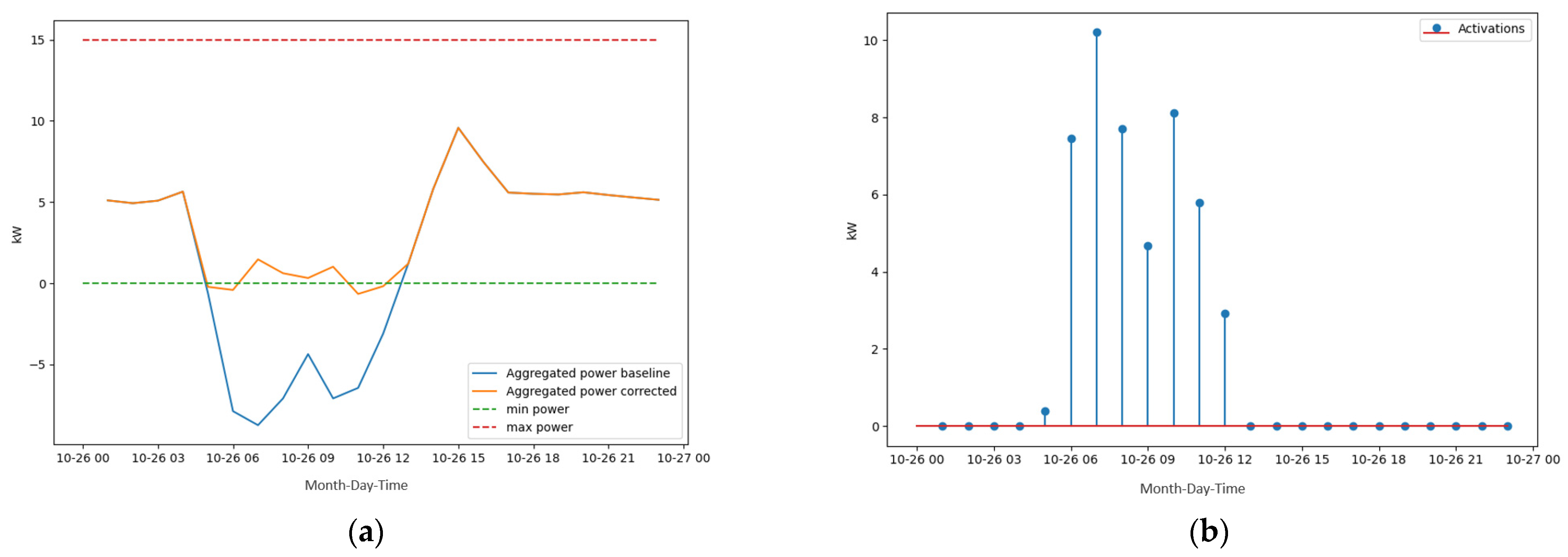
An example of the DA’s operation is presented in
Figure 3a, which shows the forecasted baseline and optimised aggregated power exchange with the grid. The baseline aggregated power (blue) has injections to the grid during the morning hours and noon. The corrected aggregated power reduces these injections, achieving close to zero consumption during those hours.
Figure 3b also shows the computed activations by the DA to correct the aggregated power.
2.4. Key Performance Indicators
The evaluation methodology aimed to deliver an overall view of the performance of an MV and LV electricity district network configuration that is connected to the electrical grid through a single connection node. In this respect, the evaluation plan with regard to the IPMVP guidelines [
28] covered the aspects of the building energy performance and the RES penetration. The following key performance indicators (KPIs) were used.
Firstly, the electric energy imported and exported from the district grid was calculated as the summation of the total electric demands of the buildings being tested. With the knowledge of the PV data, these calculations were possible. Then, the data were normalised concerning the variable-base degree-day (VBDD) method [
29]. Thus, the normalised total demand and the normalised net imported and exported energy for both the evaluation and baseline periods were calculated and then compared by computing the normalised rate of change (
):
KPIs for near-zero-electricity buildings [
30], including the load cover factor (autarky) and supply cover factor (self-consumption), were calculated. The load cover factor (
) quantifies the self-sufficiency, and is calculated as the ratio of useable electricity production (
) to the total electricity demand (
) for 15 min intervals.
The supply cover factor (
) quantifies self-consumption, and is calculated as the ratio of useable electricity production (
) to the total electricity production.
Moreover, regarding the RES penetration, the penetration of each period was estimated based on the , which expresses the percentage of the renewable production used for covering the local demand. Accordingly, the RES penetration increase was determined as the between the RES penetration of the baseline and the evaluation.
As mentioned, the KPIs were evaluated by comparing the baseline period with the results from the evaluation period and after normalisation based on the IPMVP guidelines. The period without the implementation of the solution served as a reference for the analysis of the KPIs. The VBDD method was used to normalise the buildings’ consumption from the baseline and the evaluation period. Furthermore, the factors and conditions that could affect the performance of the proposed solution were investigated in parallel with the KPIs. Significant impacts on the predictions and the overall performance can have the following factors: (i) faulty, unreliable values of the input parameters (e.g., low precision); (ii) missing input values; (iii) bad weather forecasts; (iv) communication failures; (v) physical equipment failures; (vi) occupants’ intervention; and (vii) COVID-19 impacts (e.g., safety measures). To conclude, the reflection of the influential factors on the evaluation results provided a complete overview of the proposed multilevel control approach’s performance in a district.
The thermal comfort and thermal sensation can be computed by using the predicted mean vote (PMV) and the predicted percentage of dissatisfied (PPD) (ISO 7730 [
31]):
PMV is an index that predicts the mean value of votes of a group of occupants on a seven-point thermal sensation scale. This index can be influenced by levels of physical activity, clothing insulation, and the parameters of the thermal environment. In the PMV sensation scale, +3 reflects an environment that is too hot, while −3 represents an environment that is too cold;
PPD provides the percentage of people predicted to experience local discomfort. The main factor that causes local discomfort is considered to be the unwanted cooling or heating of an occupant’s body. Influential factors include drafts, abnormally high vertical temperature differences between the ankles and head, and/or floor temperature.
All occupied areas in a space should be kept below 20% PPD to ensure thermal comfort according to the known standards (ASHRAE and ISO 7730). The thermal comfort categories are summarised in
Table 1 below.
3. Experimental Design
3.1. Case Study
Lavrion Technological and Cultural Park (LTCP) is the only technological park in Attica, and its Research and Development activities are specialised in applied technology, electronics technology, telecommunications, robotics, laser technology, environmental technology, and energy management. The park consists of 48 fully renovated buildings, 3 RES systems, 2 PV plants, 6 wind turbines, 2 energy storage systems, a battery bank with a storage capacity of 1364 Ah, a hydrogen production and storage bank able to store 1 MWh of energy, and a weather station.
All of these components are connected to the electrical grid through a single connection node, with the main MV switchboard (20 kV/50 Hz). Three MV/LV transformers with a capacity from 800 to 1250 KVA are connected to the main MV switchboard, as shown in
Figure 4.
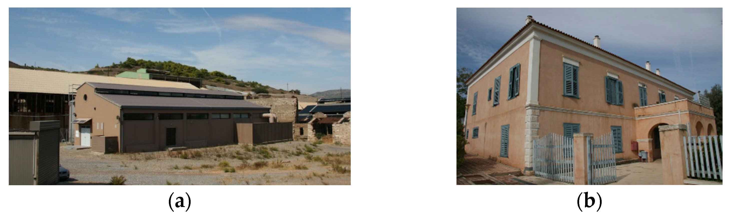
For fulfilling the experimental design purposes, the testing boundaries of LTCP include two fully controlled buildings—the H2 (active) building (143 kWh/m
2 per year) (
Figure 5a) and the admin (passive) building (92 kWh/m
2 per year) (
Figure 5b)—and two PV plants (15.1 kWp and 46.8 kWp).
The buildings are renovated, including a variety of materials in their envelope (i.e., stone, gutter tiles, concrete, bricks, etc.), and they are equipped with advanced HVAC systems. In particular, Building #1 has two separate HVAC systems; the first consists of 2 exterior variable refrigerant flow (VRF) units and 13 floor-mounted fan-coil units (maximum electrical load is approximately 25 kW). The two VRF units are able to operate either simultaneously or individually, depending on the requested load, and with a view to maximising their lifetime. The second system is a combination of an air-handling unit (AHU) and a closed-loop air/water heat pump (HP) that provides the heating/cooling demands of half of the building. The AHU ensures the recirculation of air through air ducts inside the building, with a maximum air supply of 10,000 m3/h. The total maximum electrical load of the AHU and the HP is approximately 32 kW. Building #2 has a central heating oil burner and a water boiler as well as a water chiller (25 kW), and 19 floor mounted fan-coil units.
Inside the park, there is also a variety of RES equipment that can be utilised for this test case. A PV plant with photovoltaic panels (46.8 kWp) of thin-film technology, with the efficiency of the inverters close to 98%, was selected. Additionally, photovoltaic panels (15.1 kWp) of monocrystalline cell technology with an efficiency ratio of almost 16% were included. Moreover, an online weather station is installed on the perimeter of the park. It provides measurements with a 15 min interval for ambient temperature, humidity, solar irradiance, wind speed and direction, and rainfall. The collected weather data are crucial for the development and validation of proposed solution.
The data collection, monitoring, and evaluation of the case study were performed through the deployment of more than 480 measuring points gathered to a single SQL server synchronising district and building data. The district operates under an advanced building energy management system (BEMS) that monitors the RES production and runs the control parameters of the buildings (e.g., lighting, HVAC setpoints).
3.2. Experimental Procedure
LTCP was tested under different operational schedules—residential buildings and offices, with variable PV capacities. The experimental campaign in the test site was divided into three periods, which are described in
Table 2. Firstly, this separation concerns the scaling of PV generation, which is different for each test. Secondly, it concerns the change in the environmental conditions, given that the period of September and October in Greece is distinguished by intense weather changes. This change can be observed even from the average external temperature in each period. The first period, Period 1, consisted of 28 days distributed between September and October 2020. Periods 2 and 3 consisted of 7 days each at the end of October 2020, with a colder average temperature than Period 1.
The collected data included the following:
Temperature (°C) collected from temperature sensors located inside the buildings, with a 15 min interval;
Temperature (°C), global irradiance (W/m2), and wind speed (m/s) measurements collected from the weather station, with a 15 min interval;
Energy consumed by HVAC systems (kW), determined from power meters, with a 15 min interval;
Energy generated by both photovoltaic panels (kW), determined from power meters, with a 15 min interval.
The reason for testing different scenarios was to evaluate the proposed solution for different levels of PV generation.
Figure 6 shows the configuration of the district formed at LTCP. It consists of two buildings—one active and one passive—and one PV generation station.
The BA runs every hour and produces two outputs: (1) a flexibility map for the 24 h ahead, and (2) the temperature setpoint for all fan-coil units (FCUs) in the H2 (active) building. In general, this function is performed by constantly maintaining a comfortable indoor environment for occupants, and the temperatures cannot vary by more than ±2 °C from the selected temperature setpoints. The temperature setpoints during baseline are fixed to 22 °C for both buildings. The setpoints for the FCUs are constrained to be in the set [20 °C,21 °C,22 °C,23 °C,24 °C], given by the baseline setpoint ±2 °C, to account for the quantisation of the low-level control system at LTCP.
If no activation is requested, the BA operates in its normal mode of operation. If activation is requested, the BA computes the optimal setpoint to achieve the requested activation while maintaining the thermal comfort in the building.
As mentioned above, the DA runs every hour, with an optimisation horizon of 24 h and an hourly resolution, i.e., H = 24. Going back to the optimisation problem described above, there are two buildings and two generation sources; thus, N = 2 and M = 2. The optimisation problem that the DA solves has a bound constraint of and for the power exchanged with the grid at all times. Firstly, the electric demand of the district is calculated as the summation of the total electric demands of Building #1 and Building #2. With the knowledge of the PV data, these calculations are now possible. In practice, these constraints are incorporated as soft constraints in the solver to prevent the solver from reaching unfeasible solutions in situations when is not possible to avoid injections to the grid or to have power withdrawn from the grid above 25 kW.
After the experiments, a detailed analysis was carried out for each period. The data for every experimental period (evaluation) were then compared with the data for the same period of the previous year (baseline). A key factor that must be noted is that there is a clear separation in the analysis depending on the district operating scenario. Specifically, the buildings have two operating modes, which refer to residential and office use. During residential use, the HVAC system operates 24/7 to establish the desired temperature conditions for the residents. On the other hand, during office use, the HVAC system operates only during office hours, i.e., the period between 6:00 and 18:00 (local time) for Greece. Consequently, the district also adopts these two operating modes, which are analysed separately. Thus, the data evaluated were differentiated for each scenario according to the facts mentioned above.
4. Results and Discussion
4.1. Energy Balance
The basic components of energy balance include imported energy, exported energy, and energy storage. Additionally, the total electric consumption of the buildings is essential, and consists of the imported energy from the grid and the generated energy from the RESs that were used in the buildings. The energy consumed by buildings can be influenced by several factors, including climate parameters, building envelopes, energy systems, and the behaviour of occupants, all of which must be considered for successfully identifying the energy efficiency potential and opportunities of the buildings [
32].
Regarding the two time periods (baseline and evaluation), it is worth noting that despite the implementation of the program, the consumption of the buildings in the evaluation period was several times higher than in the baseline period. This may be because of the new regulations regarding COVID-19, such as the legislation requiring the supply of 100% fresh air and no use of recirculation in the buildings, or the legislation requiring open windows throughout the day. All of these factors contribute to a massive increase in the buildings’ energy demand.
The results of the tests performed at LTCP are presented in
Table 3, and are separated by the use of the buildings and the test period (see
Table 2). In terms of total electric demand, LTCP showed an increase in its normalised consumption during the evaluation period. It is highlighted that in the first case, the consumption was extended throughout the day, whereas in the second case, the consumption was concentrated during daylight hours. Therefore, a higher potential for increasing self-consumption was found in the case of offices.
By considering the electric demand and the available PV production for each 15 min interval, the net imported and exported energy were estimated at the district level.
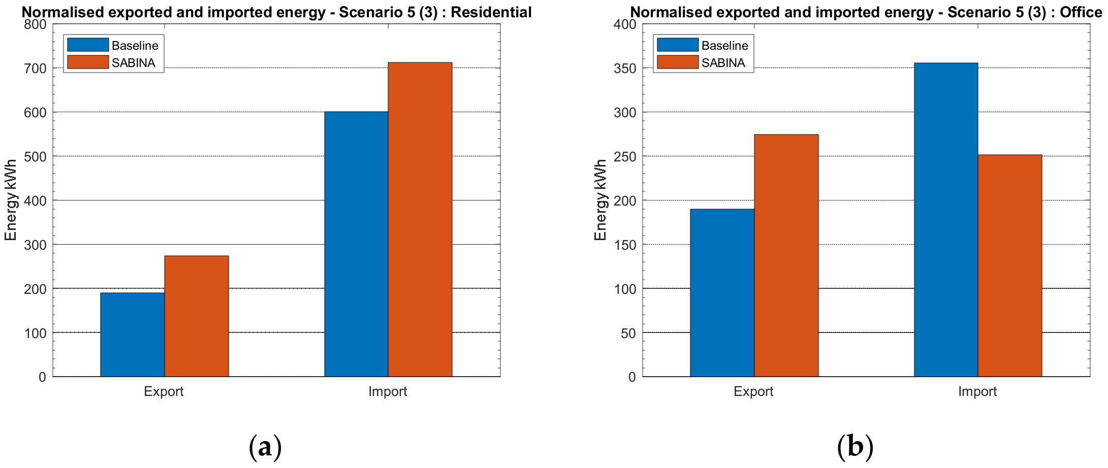
Figure 7a,b depict the normalised imported and exported energy with the grid for Period 1.
The exported energy was decreased significantly; however, the demands were increased, causing the imported energy to be increased. Even though we observed that almost all of the generated energy was consumed on-site, the energy demand of LTCP was higher during evaluation than during the baseline. This behaviour was mostly due to the mismatch in the forecasts from the different models (PV production, baseline production, etc.), which affected the optimisation of the DA, as well as the rebound effect in the afternoons/evenings due to the activations requested in the peak production hours of the PV panels (solar noon).
Figure 8a,b present the imported and exported energy for Period 2. The experiments showed that the DR solution reduced the total energy exported to the grid by 27%. All of the above can be observed in the diagrams below.
Lastly,
Figure 9a,b present the imported and exported energy for Period 3. The DR solution left the exported energy almost identical to the baseline solution. Period 3 had an average outside temperature of 18.2 °C, which is colder than the minimum zone temperature; thus, no cooling was needed during this period. This explains why the DR solution did not work properly, since the building could not deliver the requested flexibility activations by the DA. All of the above can be observed in the diagrams below.
4.2. Load Cover and Supply Cover Factors
The load and supply cover factors are indices to describe the relationship between the on-site energy generation and the buildings’ energy consumption.
Table 4 summarises the results for the LCF and SCF for both residential and office uses for all test periods.
As shown above, when the period of renewable production matches the demand of the district (office use), the benefits for the site are higher in comparison with consumption during periods with no production (residential use). The DA accomplishes a reduction in the power of the PVs, which are not used on-site significantly.
4.3. Self-Consumption
The self-consumption increase was the last KPI to be evaluated. The main objective was to increase self-consumption in the district by matching the buildings’ demand to the RES production. For this evaluation, the district was tested for the cooling period in Greece.
Table 5 summarises the self-consumption increases for residential and office use of buildings when the DA manages LTCP.
A self-consumption increase of 23.4% for the residential case and 37.1% for the office case was accomplished for the tested period. The main findings of the evaluation show that the DA accomplishes synchronisation of the input data from sites and the generated data from the models and algorithms, and delivers setpoints for the next 24 h. This optimisation provides numerous advantages for the district, including the increase in the RES penetration in the energy mix, as well as the reduction in imported energy from the electric grid. In this respect, not only the environmental footprint of the buildings, but also the operative costs for heating and cooling the buildings, are reduced.
The performance can be affected by the location and the orientation of the building (e.g., weather conditions), as well as the construction characteristics of the building (e.g., lightweight), which affect its thermal storage capacity. Furthermore, the properties and the dimensioning of the utilities and systems used (e.g., HVAC), along with the use and the schedule of the building (e.g., residential, office), can result in different beneficial opportunities, as shown from the results.
4.4. Thermal Comfort
The thermal comfort and thermal sensation depend on the physical activity that is carried out and the clothing worn, as well as on environmental parameters, e.g., air temperature, mean radiant temperature, air velocity, and humidity. Given the environmental parameters, only the temperature and, occasionally, the velocity are controlled by the HVAC. Indicatively, the results for Periods 1 (
Figure 10a), 2 (
Figure 10b), and 3 (
Figure 10c) are presented. The overall comfort level was improved for all periods, as it increased the percentage of CAT I and eliminated the occurrence of CAT IV, compared to the baseline period.
4.5. Future Research
The proposed solution aims to go beyond the state of the art and deliver services to medium- and low-voltage grids by exploiting energy storage and synergies between electric and thermal networks, and is inherently compatible with demand response. In view of this, the management algorithms are inherently capable of demand response, and prioritise the integration of renewable energy production or other controllable energy sources when available.
As observed from the results, the performance of the proposed approach and the benefits it provides to the site and the end users are linked to the building’s properties and thermal flexibility, as well as the availability of RESs and the control capability of the district. The more thermal mass a building provides, the more flexibility the system offers for thermal energy storage. In this regard, further investigation on renovating the buildings and integrating new materials is needed in order to enhance the performance of buildings towards a decarbonised and clean energy system. Phase-change materials (PCMs) are a very attractive alternative for conventional buildings’ thermal mass, including solid wood, stone, brick, gypsum, and concrete. Such materials provide high heat storage capacity within a small range of temperature change. Indicatively, for traditional internal building applications, such as walls or floors, PCMs’ phase-transition temperature is typically within the human comfort range of 20–30 °C. Therefore, improving the thermal mass of the buildings by integrating new materials, such as PCMs, can contribute to enhancing SABINA performance and reaching higher targets.
5. Conclusions
In the present work, the use of demand-side flexibility and its optimisation for exploiting distributed energy storage systems—such as buildings’ thermal mass—to constrain the energy exchange with the grid was investigated. A multilevel control algorithm was developed and validated at a district of LTCP in Greece.
The analysis was performed in accordance with the IPMVP and the KPIs defined to deliver an efficient solution to convert and store the excess renewable energy as thermal energy and, thus, provide services to both the electric grid at the building level, and the thermal grid. For the end users, management algorithms contribute to the energetic expenditure reduction of exported energy from the grid by up to 27% (based on PV availability and building-related demand). In view of this, the management algorithms are inherently capable of demand response, and prioritise the integration of renewable energy production (up to 37% increase in self-consumption) or other controllable energy sources when available. In parallel with electricity balance optimisation, the comfort level of the occupants is not only respected, but also improved to a high-standard quality (CAT I) in most cases.
This study presents great potential for RES penetration through building thermal mass exploitation. However, it should be mentioned that the case study was based on conventional buildings with high energy demand, which are not representative of the current EU buildings’ energy ratings. Renovation schemes adapting efficient insulation technologies or a building envelope embedded with high-latent-heat-capacity materials could significantly improve the activation response time and heat storage duration. At the district level, the proposed multilevel control approach transforms the building envelope into a virtual battery, which increases the grid flexibility and optimises the RES penetration. The construction industry can benefit from this technology for designing innovative building envelopes, promoting RES self-consumption, and minimising the imported energy from the grid.


 ,
, 


