Research on Anomaly Detection of Wind Farm SCADA Wind Speed Data

Abstract

Supervisory control and data acquisition (SCADA) systems are critical for wind power grid integration and wind farm operation and maintenance. However, wind turbines are affected by regulation, severe weather factors, and mechanical failures, resulting in abnormal SCADA data that seriously affect the usage of SCADA systems. Thus, strict and effective data quality control of the SCADA data are crucial. The traditional anomaly detection methods based on either “power curve” or statistical evaluation cannot comprehensively detect abnormal data. In this study, a multi-approach based abnormal data detection method for SCADA wind speed data quality control is developed. It is mainly composed of the EEMD (Ensemble Empirical Mode Decomposition)-BiLSTM network model, wind speed correlation between adjacent wind turbines, and the deviation detection model based on dynamic power curve fitting. The proposed abnormal data detection method is tested on SCADA data from a real wind farm, and statistical analysis of the results verifies that this method can effectively detect abnormal SCADA wind data. The proposed method can be readily applied for real-time operation to support an effective use of SCADA data for wind turbine control and wind power prediction.

1. Introduction

Wind energy has become one of the fastest-growing energy sources. According to the estimate by the World Wind Energy Association, by 2020, approximately 12% of the world’s electricity will be generated by wind power (GLOBAL WIND REPORT 2019). Supervisory control and data acquisition (SCADA) systems, as comprehensive monitoring systems that remotely connect each wind turbine with the main control room, have been widely used in wind power grid connection, power prediction, and wind farm operation [1,2,3] and maintenance [4]. During the operation of a wind turbine, a SCADA system typically samples wind turbine data at a high frequency (e.g., every second). Due to the high sampling frequency, SCADA data are not fully understood or utilized [5,6,7,8].

SCADA systems record numerous types of operating data, including historical operating status, and some data can be converted into characteristic curves reflecting the performance of the wind turbine, which has great utilization value [9]. High-quality SCADA data are the basis of data assimilation and post-processing of model forecasts for error correction. However, there are often abnormal data in SCADA data, including abnormal wind turbine status information, abnormal data collection, human intervention, and abnormal weather conditions. These anomalies sometimes destroy the data trends in the normal state of the wind turbine and complicate the use of data, especially for wind power prediction. Therefore, it is very important to detect and analyze anomalies in SCADA data.

At present, the prevailing methods for anomaly data detection include statistical correlation, distance relationship, deviation from physical relationship, and deviation from prediction. Anomaly detection based on statistical relationship is mainly used to test the inconsistency of each point in the sample set [10,11], finding an abnormal behavioral relationship between an individual sample and the dataset. The distance relationship method detects anomalies through the distance between a single data sample and the center of the dataset [12]. These two methods are not effective for some other complex abnormal conditions. Anomaly detection based on deviation relation is used to establish a group of data subsets of a dataset, and by calculating the dissimilarity between subsets, one can determine the outliers. In the actual data processing process, this is complex and difficult to deploy [13,14]. The method based on prediction is used to learn from a large amount of historical data, put the data into the prediction model, and compare the test data with the prediction data to confirm their abnormal characteristics [15,16]. This method sometimes assigns some normal mutation data as abnormal. For example, there are both abnormal information caused by the change in the turbine blade performance and sudden changes caused by natural severe weather. It is difficult to comprehensively detect anomalies by relying on one of the above methods alone. Therefore, this study refines and integrates three anomaly detection methods into a comprehensive detection method for filtering the abnormal SCADA data.

The rest of this article is organized as follows. In Section 2, three detection methods are introduced: the EEMD-BiLSTM network, wind speed correlation detection between adjacent wind turbines, and dynamic power curve fitting deviation detection. In Section 3, the novel design of a comprehensive detection method utilizing the three detection methods is presented, and the feasibility of the method is verified based on historical data of several wind turbines. The results of the real-time operation of the wind speed abnormality detection in the SCADA data method for a medium-sized wind farm are analyzed to determine the effectiveness of the proposed method for real-time wind speed abnormality detection in SCADA data. Finally, in Section 4, the experimental results are summarized to obtain conclusions. The major finding of this study is that the proposed detection method is capable of effectively filtering abnormal SCADA data. This method can be used for cleaning historical data records and also for real-time SCADA data quality control, effectively ensuring suitable use of SCADA data.

2. Method

2.1. EEMD-BiLSTM Network

In recent years, long short-term memory (LSTM), a deep learning technology, has been widely used in wind power prediction in the field of wind energy [17,18,19]. LSTM is a time cyclic neural network, which is specially designed to solve the long-term dependence problem existing in general RNN (Recursive Neural Network) and CNN (Convolution Neural Network).

However, using the time series model method alone, the detailed information in the data cannot be effectively displayed, so the set empirical mode decomposition method is adopted. When splitting the original signal, the decomposed components can automatically match their own scale [20]. If the decomposed components can still be split, they continue to decompose until they are not decomposed. At this time, all components of the original signal decomposed by the EEMD method have been obtained [21]. This decomposition method can mine more detailed information from inside the signal and is very suitable for dealing with unstable data. EEMD has two steps (Figure 1):

Step 1: Add normal-distributed noise to the wind speed time series to enhance EMD performance (Huang et al. [21]).

Step 2: Apply the EMD (Empirical Mode Decomposition) method to obtain N IMF (intrinsic mode components) components and a residual. This process includes obtaining the local extremum of the data, finding the upper and lower envelope of the waveform, and obtaining IMF (intrinsic mode components) by deducting the average value of the upper and lower envelope from the original time series.

The decomposition steps diagram of EEMD is shown in Figure 1.

The prediction process is shown in Figure 2 below. Firstly, the ensemble empirical mode decomposition method is used to split it into signals of different scales, so as to greatly reduce the vibration and motility of the wind speed signal. The decomposed component signals are used to optimize the parameter batch_size and the number of neurons of the Bi-LSTM model. After finding the optimal parameters, the Bi-LSTM model is initialized, and each component signal is sent to the Bi-LSTM model for training to obtain their own prediction results. The predicted wind speed is finally accumulated by the results of all components.

The EEMD-BiLSTM model is trained with SCADA data for each wind turbine independently. Figure 3 shows test results for a sample wind turbine from a mid-size wind farm located in northern Inner Mongolia. The model was trained with 10 months of data. With this short period of training data, the EEMD-BiLSTM network model can infer the true value of the wind speed with good accuracy. It can be expected that the model could be further improved with longer accumulation of data samples.

The time series anomaly detection model assumes that the observation to be detected is a missing value and uses EEMD-BiLSTM deep learning technology to estimate/project the wind speed at that time point based on the other part of the time series data, and then it is used as a reference to judge the reliability of the wind speed observed by the SCADA system. To evaluate this method, we must first evaluate the accuracy of the deep learning scheme to estimate wind speed. We used the historical observation data collected from 1 January to 31 October 2020 of a wind turbine in northern Inner Mongolia to fill in the value of the “extract and leave the missing” value of the test sample, and then compare the filled estimated wind speed with the observation to calculate the estimation accuracy. Let us use RMSE to evaluate the effect.

The RMSE is the square root of the sum of squares of the deviation between the observed and true values and the reciprocal of the number of observations (m). This parameter can be used to measure the deviation between the observed and true values. If ${\widehat{y}}^{\left(test\right)}$ represents the predicted value of the model in the testing set, then the RMSE can be expressed as:

$$RMS{E}_{test}=sqrt(\frac{1}{m}\Vert {\displaystyle \sum }_i\left({\widehat{y}}^{\left(test\right)}-y^{\left(test\right)}\right){\Vert }_i^2$$

(1)

Table 1. Root mean square error (RMSE) of the original data and the projected data under different data missing rates.

Missing Rate	RMSE
5%	0.22
10%	0.26
20%	0.48
50%	0.58

shows the statistical results for the cases of different missing rates of the data. It shows that when the missing data are within 10%, the root mean square error between the filled data and the original data is less than 0.3 m/s, indicating high accuracy.

Since there are often continuous data abnormalities in the production and operation of wind turbines, we conducted deep learning time series data estimation tests with EEMD-BiLSTM for different consecutive abnormal points.

Table 2. Root mean square error (RMSE) of original data and added data under different numbers of consecutive missing points.

Number of Consecutive Missing Points	RMSE
1	0.23
2	0.26
3	0.38
5	0.84
10	1.68

shows the experimental comparison results.

It can be seen from Table 2 that when one to three consecutive points are missing, the time series model filling data can accurately simulate the original observation data (root mean square error < 0.4 m/s), so it can be used as a reference to identify and monitor abnormal measurement data. Figure 4 shows how a time series model can be used to fill in data to monitor abnormal data points. It can be seen from the figure that this method can effectively monitor abnormal timing data.

2.2. Detection of Wind Speed Correlation between Adjacent Wind Turbines

Under the conditions of global atmospheric circulation and weather system circulation, the near-surface airflow of wind farms is determined by the local topography and other underlying surfaces, and it has a high degree of correlation over several hundred meters to several kilometers. Thus, the correlation of wind speed between two adjacent wind turbines contains crucial information on the anomalies in one or both wind turbines. The correlation analysis of wind speed between adjacent wind turbines refers to the analysis of two or more correlated variable elements to measure the closeness of the correlation between the two variable factors. The correlation coefficient reflects the direction and degree of the change trend between two variables. Its value ranges from −1 to +1, where 0 means that the two variables are not correlated. A positive value means a positive correlation, and a negative value means a negative correlation. The larger the value, the stronger the correlation.

The correlation coefficient, one of the first statistical indicators designed by statistician Carl Pearson, is a quantity measuring the degree of linear correlation between variables, usually expressed in the letter r. Due to the different study subjects, the correlation coefficient can be defined in several ways. Among them, the Pearson correlation coefficient is more commonly used.

$$r\left(X,Y\right)=\frac{Cov\left(X,Y\right)}{\sqrt{Var\left[X\right]Var\left[Y\right]}}$$

(2)

where $Cov\left(X,Y\right)$ is the covariance of $X$ and $Y$, $Var\left[X\right]$ is the $X$ variance, and $Var\left[Y\right]$ is the $Y$ variance.

The Pearson correlation analysis is widely used in the field of wind power. Selwyn [22] applied the correlation method to analyze the reliability of wind turbine components. Mostafa [23] applied wind load correlation analysis for wind farm reliability assessment. Shin [24] applied the structural correlation evaluation method of wind farms to evenly estimate the reliability of wind farms.

The wind speed correlation of two wind turbines is mainly affected by the distance between the wind turbines and the micro-scale topography of the area. First, we used the wind speed data of the wind turbines in 2019.1–2019.12 to verify the correlation. Here, we selected a medium-sized wind farm in central Mongolia, China and identified their wind speed correlation. The verification results are shown in

Table 3. Relationship between wind turbine correlation coefficients and turbine (short distance). A1–A10 are the IDs of the turbine sample.

	A1	A2	A3	A4	A5	A6	A7	A8	A9	A10
A1		0.874	0.858	0.897	0.864	0.834	0.703	0.740	0.692	0.63
A2	0.8		0.846	0.865	0.823	0.770	0.770	0.717	0.706	0.847
A3	1.03	0.23		0.818	0.806	0.767	0.850	0.612	0.675	0.815
A4	1.39	1.36	1.50		0.788	0.894	0.875	0.711	0.693	0.641
A5	1.76	1.63	1.60	2.95		0.712	0.646	0.637	0.780	0.761
A6	1.96	1.75	1.82	0.61	3.38		0.65	0.86	0.555	0.768
A7	1.97	1.30	1.20	1.38	2.73	1.23		0.639	0.519	0.818
A8	2.08	2.83	3.07	2.41	3.57	2.94	3.67		0.682	0.559
A9	2.30	2.99	3.16	3.53	2.55	4.15	4.26	2.19		0.587
A10	2.38	1.60	1.36	2.58	2.05	2.62	1.44	4.44	4.31

Note: The lower left part of the table is the distance relationship between the wind turbines, expressed in kilometers, and the upper right part of the table is the corresponding correlation relationship.

.

Table 3 and

Table 4. Relationship between wind turbine correlation coefficients and turbine (short distance). B1–B10 are the IDs of the turbine sample.

	B1	B2	B3	B4	B5	B6	B7	B8	B9	B10
B1		0.811	0.824	0.786	0.65	0.682	0.701	0.612	0.545	0.467
B2	2.72		0.745	0.801	0.711	0.648	0.622	0.601	0.568	0.531
B3	3.16	5.41		0.856	0.824	0.804	0.782	0.753	0.589	0.678
B4	4.01	6.70	2.2		0.847	0.854	0.843	0.817	0.777	0.632
B5	5.60	8.22	3.11	1.68		0.903	0.877	0.836	0.791	0.712
B6	6.45	9.02	3.75	2.60	0.93		0.893	0.813	0.754	0.697
B7	7.19	9.81	4.61	3.23	1.59	0. 88		0.887	0.743	0.654
B8	8.21	10.76	5.42	4.32	2.65	1.75	1.18		0.802	0.715
B9	10.60	13.25	8.05	6.58	5.03	4.30	3.45	2.76		0.666
B10	11.92	13.61	8.82	9.40	8.13	7.39	7.55	6.67	7.99

Note: The lower left part of the table is the distance relationship between the wind turbines, expressed in kilometers, and the upper right part of the table is the corresponding correlation relationship.

show that the wind turbines situated close to each other are highly correlated, whereas those situated farther apart are weakly correlated. Therefore, correlation of close-by wind turbines, namely, with a distance less than 3–5 km, can be used to infer the anomalies of the data of the two turbines. For a turbine of concern, by applying the algorithm to two to three close-by wind turbines, one can generally determine if the target turbine is an anomaly. In other words, if the correlation between a wind turbine and several surrounding wind turbines is very poor, this indicates that the wind turbine may be abnormal.

To demonstrate the correlation-based anomaly detection method, we selected four wind turbines (turbine A and its three adjacent turbines A1, A2, and A3) from a wind farm in northern Inner Mongolia to test the ability of our detection method to detect abnormal data. The data period used was from 1 November to 31 December 2020, and the data are the 15-min average wind speeds of the SCADA wind speed data of the four wind turbines. The calculated correlation coefficients of the four turbines are shown in

Table 5. SCADA wind speed correlation coefficients of four wind turbines.

ID	Correlation Coefficient
A1—A2	0.9834
A1—A3	0.8968
A2—A4	0.9217

.

The statistical results based on long-term (two months) samples, presented in Table 5, show that if the wind turbine is normal most of the time, the correlation between adjacent wind turbines is very good. Although there are certain differences in the correlation between different wind turbines—for example, the correlation coefficient between the A1 and A2 wind turbines and the correlation coefficient between the A1 and A3 wind turbines are relatively large—the overall result can be used by focusing on a short-term correlation, such as over the course of one to three days, to detect degrading data quality. Short-term correlation detection provides support for the quality of wind speed observation.

Table 6. Wind turbine SCADA wind speed correlation coefficient.

ID	A	A1	A2	A3
A		0.4194	0.2651	0.3087
A1	0.4194		0.8466	0.8599
A2	0.2651	0.8466		0.9160
A3	0.3087	0.8599	0.9160

shows the correlation calculation results for a three-day period.

It can be seen from Table 6 that turbine A has a poor correlation with its adjacent wind turbines A1, A2, and A3 during this period. The wind speed timing diagram of these four wind turbines during this period (Figure 5) shows that the wind speed of wind turbine A began to be abnormal at 3600 min after the start of the detection period, which is consistent with the correlation analysis result. In real-time operational applications, rolling correlation evaluation and testing of wind turbine data were performed over the past three days.

2.3. Dynamic Power Curve Fitting and Deviation Detection

2.3.1. Dynamic Power Curve Fitting

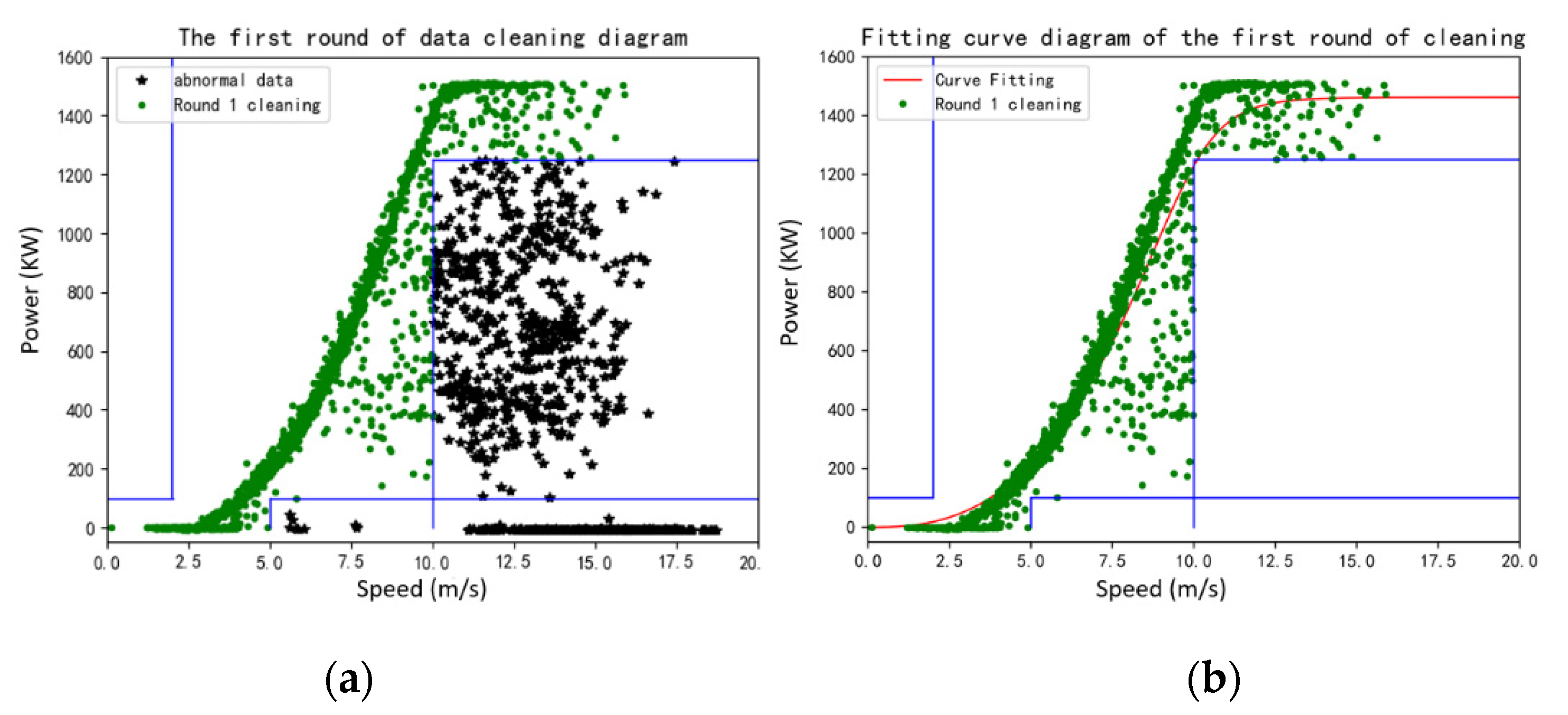
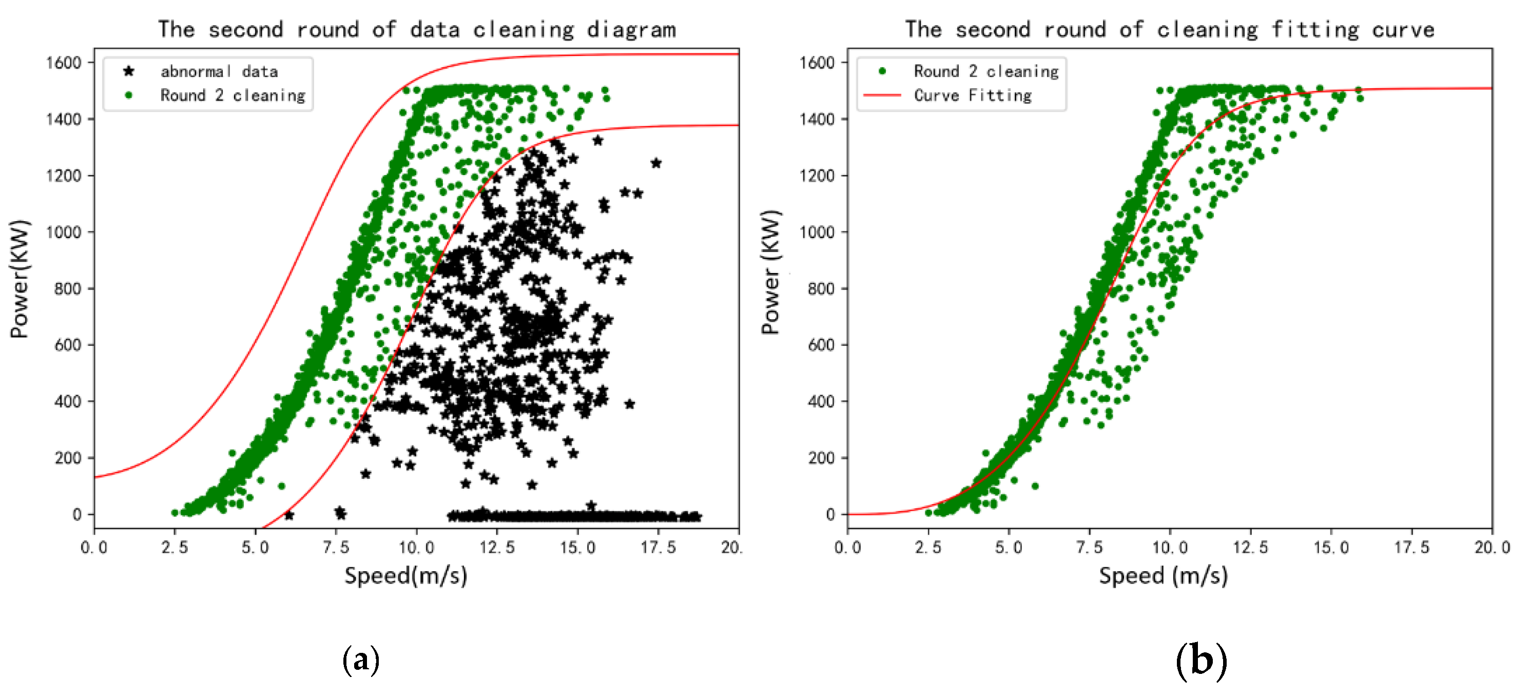
The power generated by a wind turbine is proportional to the third power of the wind speed, which satisfies a certain functional relationship, that is, a power curve. A wind turbine power curve will be provided by the wind turbine manufacturer, but due to many external factors, the actual power curve of the wind turbine installed in the wind farm will be different from the manufacturer’s calibrated power curve, and the actual power curves of identical wind turbines will not be completely consistent at different sites. SCADA wind speed and wind power monitoring data can be used to establish a dynamic power curve, which can then be used to detect abnormal wind speeds of wind turbines.

The actual power curve established based on the measured data of SCADA can be completed by the statistical fitting method. The actual power curve and the wind speed–power dispersion graph are general measures of wind turbine performance and contain important information about the overall health of the wind turbine. Many failures and performance degradation processes will be manifested in the measured power curve. The power curve generated from SCADA data can be used to detect wind turbine failures or give early indications of severe performance degradation. It also manifests abnormal SCADA data due to human interference, operation of the wind turbine, and other factors, such as icing, strong turbulence, etc.

The wind turbine power curve modeling methods of wind farms are divided into three categories, namely discrete methods, parametric methods, and non-parametric methods. Discrete methods mainly adopt a standardization algorithm based on Taylor series expansion and turbulence intensity [25]. Parametric methods mainly include the piecewise average method (IEC) [26], the piecewise linear model method [27], polynomial fitting [28], exponential fitting [29], and four-parameter logistic function [30]; non-parametric methods mainly include support vector basis, k-nearest neighbors, the decision tree, and the extreme random tree [31,32,33]. The accuracy of the parametric methods is generally worse than that of the non-parametric methods, but the parametric methods are easier to deploy. Therefore, parametric methods are often used to model the wind speed–power characteristic curve in practical applications. The three methods used in this study are described below.

(1)

Polynomial fitting method

Polynomial fitting uses polynomial expansion to fit all the observation points in the analysis area to obtain the objective analysis field of the observation data. The expansion coefficient (a) is determined by least squares fitting. For the wind speed and power data points $(x_i,y_i),1\le i\le N$ of a given wind turbine, the following n-order polynomials can be used to fit:

$$f\left(x,y\right)=a_0+a_{1}x+a_2{x}^2+\dots ={\displaystyle \sum }_{k=0}^n{a}_k{x}^k.$$

(3)

The polynomial fitting method is simple to deploy, and the power curve modeling of wind turbines currently uses polynomial fitting modeling. However, the regional polynomial fitting of this method is not stable, and missing data will cause severe distortion of the fitting curves.

(2)

Exponential fitting

The wind power curve is the most intuitive expression of the generating capacity of the unit. The power curve used for wind turbine performance analysis and evaluation is calculated from the measured wind power according to a certain algorithm.

$$p\left(v\right)=p_{max}{(1+{(\frac{\beta }{v})}^{\alpha })}^{-k}$$

(4)

where $p\left(v\right)$ is the power value, $p_{max}$ is the rated maximum power value of the wind turbine, $v$ is the wind speed value, and $\alpha$,$\beta$, and $k$ are the fitting curve parameters.

(3)

Four-parameter logic function

The shape of the curve is determined by the vector parameter $v$ = ($h$,$m$,$q$,$\tau$) of the logic function. The parameters of the logistic function can be estimated by the least square method, the maximum likelihood method, and the evolutionary programming method. Parameters can be obtained using the genetic algorithm, particle swarm optimization algorithm, and difference algorithm. The accuracy of the power curve model based on these methods is much higher than that obtained by the non-parametric method.

$$p\left(v\right)=h(1+m{e}^{-\frac{v}{\tau }}+q{e}^{-\frac{v}{\tau }})$$

(5)

(4)

Comparison of different power-curve fitting methods

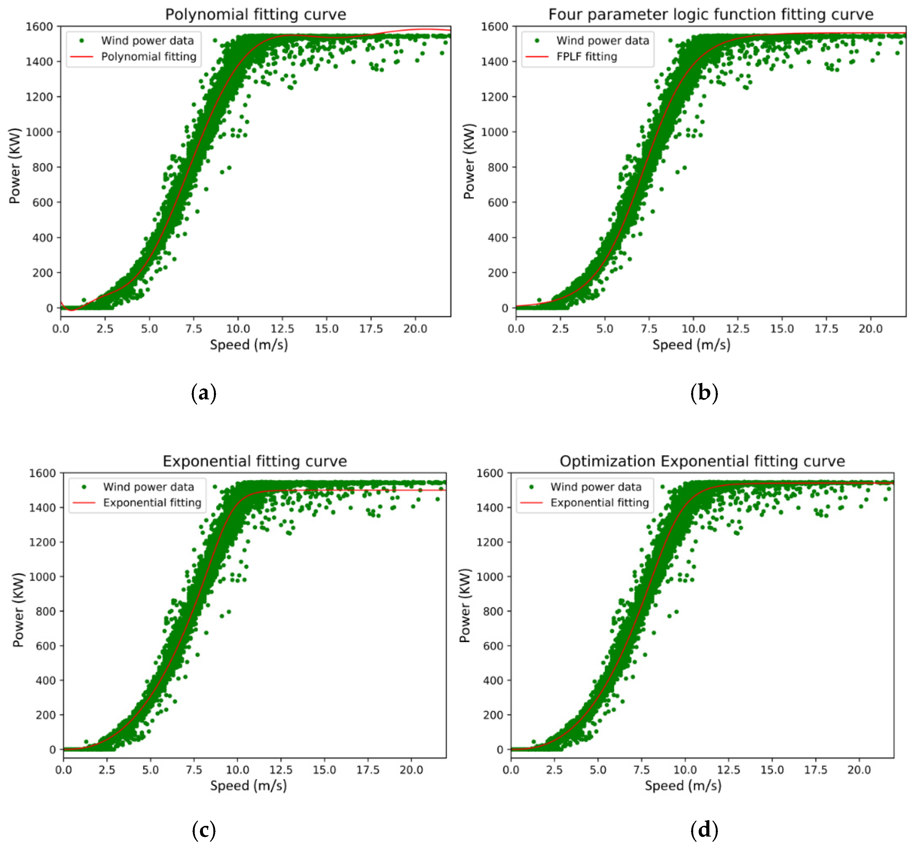
The polynomial fitting curve lacks inertia and is easily affected by abnormal data. When the wind speed reaches the maximum value and the wind speed is very small, oscillation is likely to occur. Feasible solutions require artificial reconstruction of data, which is more complicated. The four-parameter logic function is relatively more stable, but the maximum value part is prone to deviation. Non-parametric functions can better fit the wind power curve, but the relevant parameters of the fitted curve cannot be directly obtained, which is inconvenient for deployment in actual projects.

The maximum value of the curve of the exponential function method is closer to the actual curve, and there is a maximum coefficient, which can be easily determined according to the nominal power of the wind turbine or the maximum power value of the business operation. However, the maximum value of actual power may be abnormal data, so the maximum value is optimized.

$$p_{max}=p_{median}\left(p_{max-1\%}\right)$$

(6)

in which $p_{max-1\%}$ represents the power data that satisfy the wind speed—the power condition data value is in the top 1%, and $p_{median}$ represents the median of these data.

The exponential fitting formula is improved as follows:

$$p\left(v\right)=p_{median}\left(p_{max-1\%}\right) {\left(1+{\left(\frac{\beta }{v}\right)}^{\alpha }\right)}^{-k}$$

(7)

in which $p\left(v\right)$ is the power value, $v$ is the wind speed value, and $\alpha$,$\beta ,$ and $k$ are the fitting parameters. By fitting Equation (7) with the wind farm data using the Python curve_fit function, $\alpha$, $\beta$, and $k$ providing the objective function of Equation (7) and inputting historical data, the best fitting parameters are searched. The fitting curve parameters obtained by inputting one year of historical data can well reflect the curve trend.

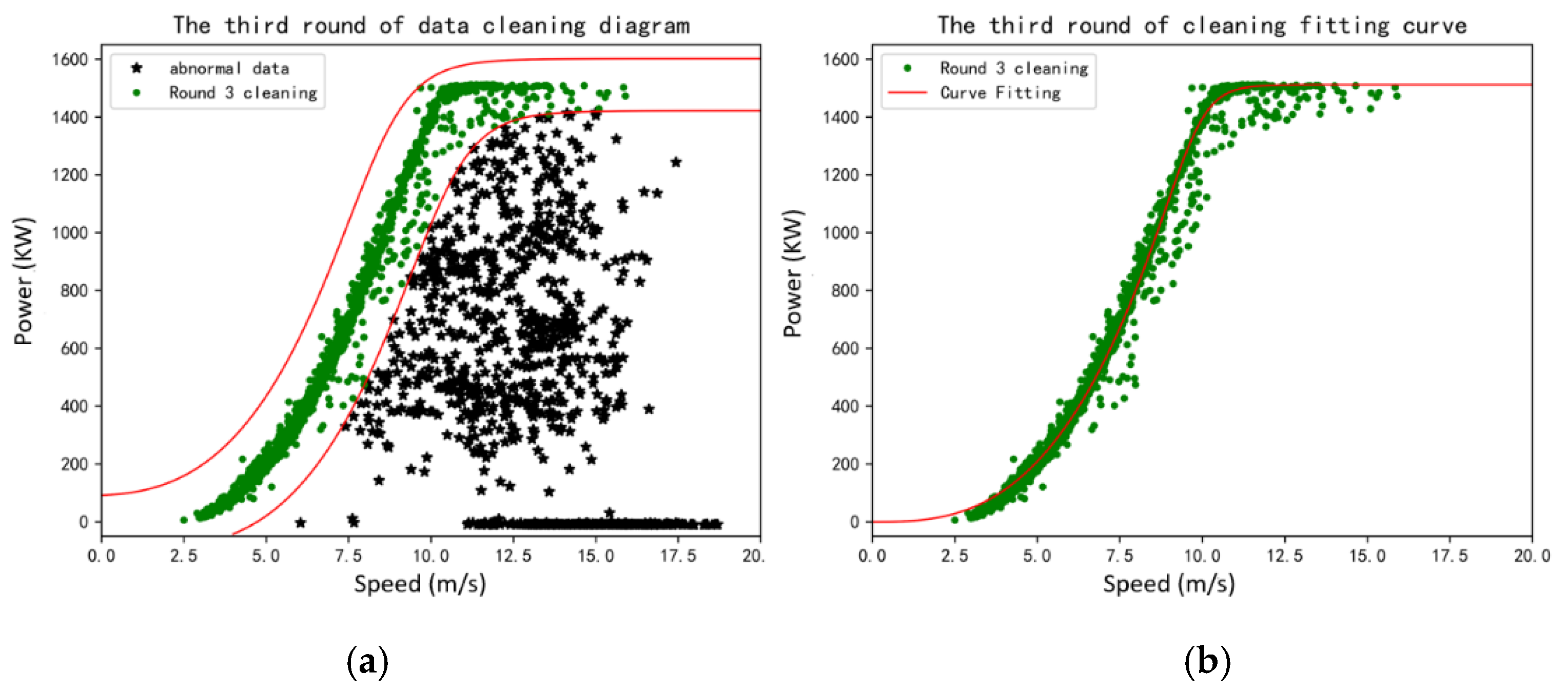
When performing power curve fitting detection, it is necessary to verify the validity of wind speed. Therefore, the power–wind speed relationship can be written as Equation (7).

$$v\left(p\right)=\frac{\beta }{{({\left(\frac{p_{max}}{p}\right)}^{\frac{1}{k}}-1)}^{\frac{1}{\alpha }}}$$

(8)

For the purpose of comparison, the above methods are employed to fit the same data of a wind turbine with a rated power of 1500 kW in the selected wind farm in northern Inner Mongolia, and the fitting results are shown in Figure 6.

Table 7. Fitting parameters of four power curve methods and standard deviation (STD).

Method Name	Estimated Power Curve Model	STD
Polynomial fitting curve	$\begin{array}{c}\hfill p\left(v\right)=(1.818525e-07)v^{12}+(-2.087167e-07)v^{11}+(0.001049e-07)v^{10}\\ \hspace{1em}\hspace{1em}\hspace{1em}\hspace{1em}\hspace{1em}\hspace{1em}+(-0.030400e-07)v^9+(0.560398e-07)v^8+(-6.864335e\hfill \\ \hspace{1em}\hspace{1em}\hspace{1em}\hspace{1em}\hspace{1em}\hspace{1em}-07)v^7+(56.650744e-07)v^6+(-312.860432e-07)v^5\hfill \\ \hspace{1em}\hspace{1em}\hspace{1em}\hspace{1em}\hspace{1em}\hspace{1em}+(1124.427590e-07)v^4+(-2481.557522e-07)v^3\hfill \\ \hspace{1em}\hspace{1em}\hspace{1em}\hspace{1em}\hspace{1em}\hspace{1em}+(3010.529090e-07)v^2+(-1536.384914e-07)v^1\hfill \\ \hspace{1em}\hspace{1em}\hspace{1em}\hspace{1em}\hspace{1em}\hspace{1em}+(40.998947e-07)\hfill \end{array}$	100.71
Four parameter logic function fitting curve	$p\left(v\right)=40.583958(1+0.001335e^{-\frac{v}{0.642477}}+7.120038e^{-\frac{v}{0.642477}})$	112.26
Exponential fitting curve	$p\left(v\right)=1500{(1+{\left(\frac{0.018541}{v}\right)}^{1.527456})}^{-8534.785265}$	94.97
Optimization exponential fitting curve	$p\left(v\right)=1512.0{(1+{\left(\frac{0.018571}{v}\right)}^{1.508083})}^{-7657.954055}$	92.80

gives the trained parameters of the four curve-fitting methods and the corresponding standard deviation. Although the optimized exponential fitting method does not significantly improve the STD compared with the polynomial fitting method, it has fewer control parameters and is convenient for practical deployment.

Figure 6 shows that in a well-performed wind turbine, all methods achieve reasonably good fitting curves, although there are evident differences in the wind ranges below the turbine cut-in speed and above label power capacity.

2.3.2. Mahalanobis Distance

Since the unit scale of wind speed and power is inconsistent, a Mahalanobis distance pair is used to describe the similarity relationship between points. It is an effective method to calculate the similarity of two unknown sample sets. Unlike Euclidean distance, it considers the relationship between various characteristics.

If two vectors, $x_1,x_2\in R,$ are two groups of samples of the dataset, U is the mean of vector $x_1$, V is the mean of vector $x_1$, and Σ is the covariance of $x_1$ and $x_2$, the Mahalanobis distance between $x_1$ and $x_2$ is:

$$Di{s}_{\mathrm{Mahalanobis}}(x_1,x_2)=\sqrt{{\left(x_1-U\right)}^T{\mathsf{\Sigma }}^{-1}\left(x_2-V\right)}$$

(9)

Table 8. Table of relationship between distance and points.

Mahalanobis Distance	Percentage of Distance Range Content Points
0.5	30%
0.9	70%
1.5	90%
2	93%
3	94%

shows that if the Mahalanobis distance is 1.5, a better retention point can be obtained. When the distance is greater than 2, the number of the retention points changes little.

2.3.3. Power–Curve Deviation Abnormal Data Detection

For data quality control, it is important to note that one should not use all data of a wind turbine for fitting its power curve. If one does, and if there is a significant amount of abnormal data, the generated fitting curve (e.g., the red curve shown in Figure 7 for a selected turbine) will not contain useful information for the deviation detection requirements.

To solve the problem, a multi-step dynamic power fitting method was implemented. Firstly, based on the wind turbine operating mechanism and operating strategy, a coarse-grained confidence equivalent wind speed boundary model was established to identify and eliminate obvious abnormalities, that is, “power curve impossible” data. The cleaning process is shown in Figure 8.

The diagram on the left in Figure 8 illustrates the first round of cleaning data. The blue box indicates the “impossible power curve area”, which is directly eliminated. The diagram on the right in Figure 8 shows the data fitting after the first round of cleaning, where the red line is the power curve generated using the cleaned data. The power curve generated by the data after the first round of cleaning better reflects the power curve. Based on the first-round fitted wind power curve, we performed the second step of cleaning to improve the accuracy of the power curve. The setting method is to substitute the SCADA data power value into the first fitting curve to calculate the wind speed. The wind speed value in the SCADA data is within the range of ±2 when the wind speed value in the SCADA data is in the range of ±2. A wind farm verifies that the restriction conditions used in the second round of cleaning are reasonable. The fitting curve after cleaning is shown in Figure 9.

The diagram on the left side of Figure 9 illustrates the second-round data cleaning algorithm. The black points are the abnormal data points, which are directly eliminated. The diagram on the right side of Figure 9 shows the data fitting after the second round of cleaning, where the red line is the power curve generated using the cleaned data. After the second step of data cleaning, the fitted power curve is more accurate. The third step is to repeat the cleaning process of the second step based on the wind power curve fitted in the second step. The setting method is to substitute the SCADA data power value into the second fitting curve to inversely calculate the wind speed. If the wind speed value in the SCADA data is within the range of ±1.5 for the inverse wind speed value, the data are considered normal. The process is shown in Figure 10.

The diagram on the left side of Figure 10 shows the third round of data cleaning. The black points are designated as the abnormal data points. The diagram on the right side of Figure 10 shows the data fitting after the third round of cleaning, where the red line is the power curve generated using the cleaned data. After the third step of data cleaning, the fitted power curve much accurately expresses the wind speed and power relationship of the wind turbine.

The advantage of dynamic power curve fitting is that it can accurately fit the wind speed–power function relationship of wind turbines in the normal operation state of wind farms and readily support monitoring of wind turbine performance and aid in quality control of wind turbine SCADA wind speed data. In practical applications, it is necessary to experimentally determine the data length (time period) and update frequency for power curve fitting. The length of the time period must meet the representative requirement of number of data samples for the power curve fitting, and the update frequency is mainly affected by seasonal changes in the performance of the wind turbine mechanical equipment and meteorological conditions. Based on the wind farm selected for this study, the SCADA data of the past two months can meet the requirements, and the frequency of updating the fitting can be up to a month.

3. Evaluation of Real-Time Application

3.1. Summary of Data

In this study, SCADA data obtained from a real wind farm in northern Inner Mongolia were used to evaluate the proposed detection method. The wind farm is located in mountainous with steep terrain, and there are 42 wind turbines distributed along the ridges of the terrain at heights of around 1770–1960 m. The distribution of wind turbines is shown in Figure 11. We note that due to proprietary requirements, the geophysical information (e.g., latitude and longitude) of the wind turbines and the domain are not shown. The data include 15-min average wind speed and power output from 1 January to 31 October 2020 for all 42 wind turbines.

3.2. Evaluation Method

A two-class confusion matrix (

Table 9. Table of contingencies.

The True Situation	Test Result (Positive)	Test Result (Negative)
Positive	True positive (TP)	False negative (FN)
Negative	False positive (FP)	True negative (TN)

) is used to quantitatively assess the anomaly detection state.

Based on the matrix in Table 9, the following three statistical scores can be calculated:

(1)

Precision

Precision is defined as follows:

$$Precision=\frac{TP}{TP+FP}$$

(10)

Precision shows a ratio of correctly detected anomaly samples over the total detected anomaly samples.

(2)

Recall

Recall is defined as follows:

$$Recall=\frac{TP}{TP+FN}$$

(11)

Recall is the proportion of the number of anomalies correctly detected to the actual number of anomalies in the testing dataset.

(3)

F1-Score

These quantities are also related to the F1-Score, which is defined as the harmonic mean of precision and recall:

$$F1=2\times \frac{Precision\times Recall}{Precision+Recall}$$

(12)

The system can obtain a high precision score while a number of anomalies are being missed. Similarly, the system can obtain a high recall score, while the false positive rate is higher. Therefore, the F1-score provides more general information on the accuracy of the proposed approach because it is the weighted average of the precision and recall rates.

3.3. Evaluation Results

In this section, we present the results of the three anomaly detection schemes and the combined approach. The data period is from 1 November 2020 to 31 December 2020, with a total of 245,952 15-min mean value samples.

3.3.1. Efficiency of the Three Detection Methods

EEMD-BiLSTM Correlation and Power Curve based abnormal data detection methods attempt to identify anomaly data from very different perspectives of the SCADA data. The EEMD-BiLSTM model can detect sudden abnormal information of the wind turbine in the time series, but it cannot effectively detect abnormal changes in wind speed trends or abnormal data that do not meet the normal state of the wind turbine. It can be seen from the statistics in

Table 10. Detection of abnormal situations from SCADA data.

Method	Total Number of Wind Data Sample	Detected Anomaly Points	Failed to Detect Abnormal Points	Detection Ratio
EEMD-BiLSTM	691,200	17,646	30,046	0.37
Correlation	691,200	31,476	16,216	0.66
Power curve fitting	691,200	12,400	35,292	0.26

that correlation detection can find a larger proportion of the abnormal data, but the other two methods cannot effectively find abnormal data. Therefore, it is difficult to comprehensively monitor all abnormalities using the three methods individually.

A combined application of the EEMD-BiLSTM model, the wind speed correlation detection approach, and dynamic power curve fitting and deviation detection algorithm would enable an effective integrated anomaly detection model. Figure 12 lays out the dataflow of the combination scheme that allows the three methods to collaboratively discover abnormal data.

3.3.2. Overall Evaluation

For an overall evaluation, all 42 stably running wind turbines of a medium-sized wind farm were selected for evaluating the abnormal wind speed detection methods. The data from 1 January 2019 to 31 October 2020 were selected for training the models, and the data from 1 November 2020 to 31 December 2020 were for anomaly detection test. We computed the Precision, Recall, and F1-Score of the individual analysis of the three anomaly detection methods developed in this study and their combined usage. The results are presented in

Table 11. Comparison of anomaly data detected by the proposed combined approach with the individual approaches.

Method	Precision	Recall	F1-Score
EEMD-BiLSTM	0.3699	0.8976	0.5239
Correlation	0.6599	0.9967	0.7940
Curve fitting	0.2600	0.9947	0.4122
Combined approach	0.9125	0.9978	0.9532

. The table shows that the correlation detection method gains the best precision, while the F1-Scores of the three methods are close. However, the combined approach, with use of the three methods collaboratively, yields significantly superior performance.

4. Summary and Conclusions

There are many reasons for and different manifestations of SCADA data abnormalities, and a single detection method cannot effectively and comprehensively evaluate abnormal conditions. This study introduces a method for detecting the quality and anomalies of SCADA data with a combined approach based on EEMD-BiLSTM deep learning data fitting anomaly detection, correlation anomaly detection, and dynamical power-curve fitting anomaly detection. The characteristics and performance of the anomaly detection approaches are studied with wind farm SCADA data. The main conclusions of this study are as follows:

(1)

The wind speed correlation detection of nearby wind turbines can be used to effectively determine whether the wind speed data are abnormal for a certain period, but it cannot be used to determine individual data abnormalities.

(2)

The wind power curve is effective to determine whether the discrete wind speed point value is in line with the rated generation of the wind turbine, but it is less useful for weak winds (less than the cut-in wind speed) and strong winds (larger than the wind speed of the rated power). It also requires continuous monitoring of the overall health of wind turbines to make sure the automatic power-curve fitting is working properly.

(3)

The EEMD-BiLSTM model can be used to determine whether the wind speed value meets the time series law, but it is only effective for short-term abnormalities.

(4)

Through the coordinated combined monitoring of the three methods, abnormalities of SCADA data can be effectively detected.

The SCADA anomaly detection method developed in this study can be readily deployed for real time uses. It has been applied by the Inner Mongolia Electric Power Company, China, for real-time operation, and the system plays a critical role for supporting the data assimilation and model output bias correction of a numerical weather prediction model operated by the company for wind forecasting at over 100 wind farms.

References

1. Zhao, Y.; Li, D.; Dong, A.; Kang, D.; Lv, Q.; Shang, L. Fault Prediction and Diagnosis of Wind Turbine Generators Using SCADA Data. Energies 2017, 10, 1210. [Google Scholar] [CrossRef]
2. Kong, Z.; Tang, B.; Deng, L.; Liu, W.; Han, Y. Condition monitoring of wind turbines based on spatio-temporal fusion of SCADA data by convolutional neural networks and gated recurrent units. Renew. Energy 2020, 146, 760–768. [Google Scholar] [CrossRef]
3. Qiu, Y.; Feng, Y.; Infield, D. Fault Diagnosis of Wind Turbine with SCADA Alarms Based Multidimensional Information Processing Method. Renew. Energy 2019, 145, 1923–1931. [Google Scholar] [CrossRef]
4. GWEC. GWEC|Global Wind Report 2019. 2020. Available online: https://gwec.net/global-wind-report-2019/ (accessed on 9 September 2021).
5. Zaher, A.S.A.E.; McArthur, S.D.J.; Infield, D.G.; Patel, Y. Online wind turbine fault detection through automated SCADA data analysis. Wind Energy 2010, 12, 574–593. [Google Scholar] [CrossRef]
6. Schlechtingen, M.; Santos, I.F.; Achiche, S. Wind turbine condition monitoring based on SCADA data using normal behavior models. Part 1: System description. Appl. Soft Comput. 2013, 13, 259–270. [Google Scholar] [CrossRef]
7. Uluyol, O.; Parthasarathy, G.; Foslien, W.; Kim, K. Power Curve Analytic for Wind Turbine Performance Monitoring and Prognostics. In Proceedings of the Annual Conference of the Prognostics and Health Management Society, Montreal, QC, Canada, 25–29 September 2011; pp. 1–8. [Google Scholar]
8. Yang, W.; Court, R.; Jiang, J. Wind turbine condition monitoring by the approach of SCADA data analysis. Renew. Energy 2013, 53, 365–376. [Google Scholar] [CrossRef]
9. Lin, Z.; Liu, X.; Collu, M. Wind power prediction based on High-frequency SCADA data along with isolation forest and deep learning neural networks. Int. J. Electr. Power Energy Syst. 2020, 118, 105835. [Google Scholar] [CrossRef]
10. Yu, S.; Li, X.; Chen, S.; Zhao, L. Exploring the Intrinsic Probability Distribution for Hyperspectral Anomaly Detection. Remote Sens. 2021, 14, 441. [Google Scholar] [CrossRef]
11. He, Z.; Xu, X.; Deng, S. Discovering cluster-based local outliers. Pattern Recognit. Lett. 2003, 24, 1641–1650. [Google Scholar] [CrossRef]
12. Pang, G.; Yan, C.; Shen, C.; Hengel AV, D.; Bai, X. Self-Trained Deep Ordinal Regression for End-to-End Video Anomaly Detection. In Proceedings of the IEEE/CVF Conference on Computer Vision and Pattern Recognition, Seattle, WA, USA, 13–19 June 2020. [Google Scholar]
13. Hu, W.; Gao, J.; Li, B.; Wu, O.; Du, J.; Maybank, S. Anomaly Detection Using Local Kernel Density Estimation and Context-Based Regression. IEEE Trans. Knowl. Data Eng. 2020, 32, 218–233. [Google Scholar] [CrossRef]
14. Wu, X.; Shi, B.; Dong, Y.; Huang, C.; Faust, L.; Chawla, N.V. Restful: Resolution-aware forecasting of behavioral time series data. In Proceedings of the 27th ACM International Conference on Information and Knowledge Management, Torino, Italy, 22–26 October 2018; pp. 1073–1082. [Google Scholar]
15. Su, Y.; Zhao, Y.; Niu, C.; Liu, R.; Sun, W.; Pei, D. Robust Anomaly Detection for Multivariate Time Series through Stochastic Recurrent Neural Network. In Proceedings of the KDD ’19: 25th ACM SIGKDD International Conference on Knowledge Discovery & Data Mining, Anchorage, AK, USA, 4–8 August 2019. [Google Scholar]
16. Zong, B.; Song, Q.; Min, M.R.; Cheng, W.; Lumezanu, C.; Cho, D.; Chen, H. Deep Autoencoding Gaussian Mixture Model for Unsupervised Anomaly Detection. In Proceedings of the International Conference on Learning Representations, Vancouver, BC, Canada, 30 April–3 May 2018. [Google Scholar]
17. Yalan, H.; Liang, C. A nonlinear hybrid wind speed forecasting model using LSTM network, hysteretic ELM and Differential Evolution algorithm. Energy Convers. Manag. 2018, 173, 123–142. [Google Scholar]
18. Chen, M.R.; Zeng, G.Q.; Lu, K.D.; Weng, J. A Two-Layer Nonlinear Combination Method for Short-Term Wind Speed Prediction Based on ELM, ENN and LSTM. IEEE Internet Things J. 2019, 6, 6997–7010. [Google Scholar] [CrossRef]
19. Memarzadeh, G.; Keynia, F. A new short-term wind speed forecasting method based on fine-tuned LSTM neural network and optimal input sets. Energy Convers. Manag. 2020, 213, 1–15. [Google Scholar] [CrossRef]
20. Jaseena, K.U.; Kovoor, B.C. Decomposition-based hybrid wind speed forecasting model using deep bidirectional LSTM net-works. Energy Convers. Manag. 2021, 234, 113944. [Google Scholar] [CrossRef]
21. Huang, N.E.; Shen, Z.; Long, S.R.; Wu, M.C.; Shih, H.H.; Zheng, Q.; Yen, N.-C.; Tung, C.C.; Liu, H.H. The empirical mode decomposition and the Hilbert spectrum for nonlinear and non-stationary time series analysis. Proc. R. Soc. A Math. Phys. Eng. Sci. 1998, 454, 903–995. [Google Scholar] [CrossRef]
22. Selwyn, T.S.; Kesavan, R. Reliability Analysis of Sub Assemblies for Wind Turbine at High Uncertain Wind. In Advanced Materials Research; Trans Tech Publications Ltd.: Bäch, Switzerland, 2012; pp. 1121–1125. [Google Scholar]
23. Hosseinpour, M.; Rajabi Mashhadi, H.; Hajiabadi, M.E. A probabilistic model for assessing the reliability of wind farms in a power system. J. Zhejiang Univ. Sci. C 2013, 14, 464–474. [Google Scholar] [CrossRef]
24. Shin, J.S.; Kim, J.O.; Cha, S.T.; Wu, Q. Reliability evaluation considering structures of a large scale wind farm. In Proceedings of the Power Electronics and Applications (EPE), 15th European Conference on IEEE, Lille, France, 2–6 September 2013; pp. 2–6. [Google Scholar]
25. Ling, W.N.; Han, N.S.; Li, R.Q. Short-term wind power forecasting based on cloud SVM model. Electr. Power Autom. Equip. 2013, 33, 34–38. [Google Scholar]
26. Thapar, V.; Agnihotri, G.; Seth, V.K. Critical analysis of methods for mathematical modeling of wind turbines. Renew. Energy 2011, 36, 3166–3177. [Google Scholar] [CrossRef]
27. Lydia, M.; Selvakumar, A.I.; Kumar, S.S.; Kumar, G.E.P. Advanced algorithms for wind turbine power curve modeling. IEEE Trans. Sustain. Energy 2013, 4, 827–835. [Google Scholar] [CrossRef]
28. Trivellato, F.; Battisti, L.; Miori, G. The ideal power curve of small wind turbines from field data. J. Wind. Eng. Ind. Aerodyn. 2012, 107, 263–273. [Google Scholar] [CrossRef]
29. Marčiukaitis, M.; Žutautaitė, I.; Martišauskas, L.; Jokšas, B.; Gecevičius, G.; Sfetsos, A. Non-linear regression model for wind turbine power curve. Renew. Energy 2017, 113, 732–741. [Google Scholar] [CrossRef]
30. Feijoo, A.; Villanueva, D. Four parameter models for wind farm power curves and power probability density functions. IEEE Trans. Sustain. Energy 2017, 8, 1783–1784. [Google Scholar] [CrossRef]
31. Ouyang, T.; Kusiak, A.; He, Y. Modeling wind-turbine power curve: A data partitioning and mining approach. Renew. Energy 2017, 102, 1–8. [Google Scholar] [CrossRef]
32. Janssens, O.; Noppe, N.; Devriendt, C.; Van de Walle, R.; Van Hoecke, S. Data-driven multivariate power curve modeling of offshore wind turbines. Eng. Appl. Artif. Intell. 2016, 55, 331–338. [Google Scholar] [CrossRef]
33. Gill, S.; Stephen, B.; Galloway, S. Wind turbine condition assessment through power curve Copula modeling. IEEE Trans. Sustain. Energy 2012, 3, 94–101. [Google Scholar] [CrossRef]
Figure 1. The decomposition steps diagram of EEMD.
Energies 15 05869 g001
Figure 2. EEMD−BiLSTM model prediction flow chart.
Energies 15 05869 g002
Figure 3. An example of time series projection of wind speed by the Bi-LSTM model.
Energies 15 05869 g003
Figure 4. Sample result of EEMD-BiLSTM Anomaly data detection for a wind turbine.
Energies 15 05869 g004
Figure 5. The SCADA wind speed (72 h) change sequence diagram of the four selected wind turbines in the northern Inner Mongolia wind farm (cf. Figure 11).
Energies 15 05869 g005
Figure 6. Comparison of wind power fitting curves (red curve). The green dots are 15-min mean wind speed and wind power pairs. The data period is 1 January 2019 to 1 November 2019. (a) Polynomial fitting curve; (b) four parameter logic function fitting curve; (c) exponential fitting curve; (d) optimization exponential fitting curve.
Energies 15 05869 g006
Figure 7. SCADA wind speed and power data fitting diagram for a sample wind turbine. The power curve is shown in red. The green dots are 15-min mean wind speed and wind power pairs. The data period is 1 January 2019 to 31 December 2019.
Energies 15 05869 g007
Figure 8. Same as Figure 7, but for the first round of data cleaning and power curve fitting. labels (a): Areas (blue frames) of “power curve impossible” data (black dots) are marked and removed; labels (b) power curve fitting (red curve) after removing the bad data. (a) The first round of data cleaning diagram; (b) fitting curve diagram of the first round of cleaning. The blue lines enclose the areas of “impossible power curve area” determined empirically.
Energies 15 05869 g008
Figure 9. Same as Figure 8, but for the second round of data cleaning and power curve fitting. (a) The second round of data cleaning diagram; (b) the second round of cleaning fitting curve. The red lines in (a) enclose the area in which the wind speeds of the data samples deviate from the power curve obtained in Figure 8b by less than 2 m/s. The red lines in (b) are the refined power curve.
Energies 15 05869 g009
Figure 10. Same as Figure 8 but for the third round of data cleaning and power curve fitting. (a) The third round of data cleaning diagram; (b) the third round of cleaning fitting curve.
Energies 15 05869 g010
Figure 11. Distribution of wind turbines used for real-time study. The color shades show the terrain height (meters above sea level).
Energies 15 05869 g011
Figure 12. Framework of the integration of the collaborative anomaly detection schemes.
Energies 15 05869 g012