3D Fracture Propagation Simulation and Pressure Decline Analysis Research for I-Shaped Fracture of Coalbed

Abstract

After hydraulic fracturing, some treatments intended for production enhancement fail to yield predetermined effects. The main reason is the insufficient research about the fracture propagation mechanism. There is compelling evidence that I-shaped fracture, two horizontal fractures at the junction of coalbed and cover/bottom layer, and one vertical fracture in the coalbed have formed in part of the coalbed after hydraulic fracturing. Therefore, this paper aims at I-shaped fracture propagation simulation. A novel propagation model is derived on the basis of a three-dimensional (3D) model, and the coupling conditions of vertical fracture and horizontal fractures are established based on the flow rate distribution and the bottom-hole pressure equality, respectively. Moreover, an associated PDA (pressure decline analysis of post-fracturing) model is established. Both models complement with each other and work together to guide fracturing treatment. Finally, a field case is studied to show that the proposed models can effectively investigate and simulate fracture initiation/propagation and pressure decline.

1. Introduction

Hydraulic fracturing (HF) can be defined as the process of fracture initiation and propagation. It is the process of squeezing liquid into the fracture through hydraulic action [1]. Today, HF is an effective means to improve the production of oil and gas wells in the field of petroleum industry [2]. As a result of HF in a coal seam, artificially induced fractures appear, and permeability increases. In the meantime, high pressure fluid can squeeze out the gas in the coal seam, which can release and absorb the gas around the well to increase the total gas volume [3]. However, not all measures can achieve the expected effect in the production after coal seam fracturing [4,5]. Research on new fracture propagation mechanisms and models will provide more methods and effective guidance for analyzing and solving this problem. Promote the output after fracturing treatment to meet the expectation.

On the basis of theoretical and field experimental work on fracture propagation mechanism, vertical fracture and horizontal fractures coexist in coal seam after fracturing [6]. In this kind of complex fracture, T-shaped and I-shaped fracture are special shapes [7,8]. The mutual influence of many factors leads to this phenomenon, such as the existence of the coalbed cleats at the interface of coalbed and cover/bottom layer [9], the large differences in the mechanical properties between coalbed and cover/bottom layer, tectonic stress of coal seams, coal blockage, interface effects of different lithologies [10,11], etc. The T-shaped and I-shaped fracture have been found in some realistic areas, and they were directly observed after HF [12]. Meanwhile, Guo et al. [13] and Tang et al. [14] have proved the existence of these kinds of fractures. Hence, correct understanding the propagation mechanism of these kinds of fracture is essential for fracturing effects.

Several models have been developed to describe the fracture propagation during HF before, such as 2D fracture models, P3D models, and fully three-dimensional (F3D) models. These models describe the propagation of vertical fracture or horizontal fracture and are also the basis for studying the propagation of I-shaped fracture. Before the 1980s, the study of fracture propagation used 2D fracture models, such as the PKN [15], KGD [16], and Penny [17] models. PKN is the basis of various complex models [18], which can still play an excellent effect on some specific problems [19]. The 2D model is a simple and fast alternative tool, but the effect is not very good because it can not simulate the propagation of fracture in horizontal and vertical directions at the same time [20]. Scholars proposed a variety of P3D fracture models and two F3D fracture models based on the past study. Developed from the 2D models, the 3D models assume that the height increases with fracturing time and varies along the propagating direction. P3D models have been widely used [21,22,23]. Guo et al. [9] and Dontsov et al. [24] have researched and developed the P3D fracture model. Zhang et al. [25] distinguished the material properties and in-situ stress of the conventional model, and proposed a new quasi three-dimensional model with its numerical solution. Zia and Lecampion [26] proposed an open-source simulator of P3D model on Python and gave a series of numerical examples. Aiming at the problem that it was difficult to couple hydraulic fracturing with proppant transportation, Skopintsev et al. [27] proposed an enhanced P3D model. Linkov and Markov [28] combined KGD with P3D to obtain an improved P3D model, which is more perfect in considering in-situ stress. Wen et al. [29] considered the rheology and filtration of fracturing fluid, improved the PKN model, and obtained a new P3D model. The even more complex F3D models can produce better results. Clifton et al. and Lam established the F3D models respectively and had developed them later [30,31]. The F3D models are more rigorous in mathematics, but the operation cost is much higher. For complex fractures, Karimi-Fard et al. [32] and Hossain et al. [33] established fracture simulation models for fracturing of shale gas and tight gas reservoir, respectively. Wu et al. [9] and Cheng et al. [8] established a 2D mathematical model of the T-shaped fracture of the coalbed and solved this model, but it is limited to the 2D plane-strain conditions, which is different from actual situation. In addition, the complex fracture models based on displacement discontinuity method (DDM) and embedded discrete fracture model (EDFM) can also address the fracture geometries [34,35,36]. However, these models are aimed at complex fracture networks, which are not suitable for the I-shaped fracture studied in this paper. Moreover, the conventional fracture models mentioned above can also be used as the basis for the study of I-shaped fracture, but they can not directly solve the problem of the propagation simulation of it.

It is well known that simulation of fracture propagation and simulation of PDA are two important tools for calculating the geometric sizes and mastering the dynamic propagation laws of fractures [37]. Both methods support and complement with each other, and work together to guide fracturing treatment. Therefore, the goal of this work is to establish propagation simulation model and PDA model based on the propagation mechanism of I-shaped fracture. The T-shaped fracture can be solved by the similar method. Guo et al. [38,39] and Zhao et al. [40] had proposed the P3D model of PDA, and obtained a series of research results. However, the PDA models which have existed are just for conventional fractures (vertical fracture or horizontal fracture). There has been no satisfactory model for the I-shaped fracture so far.

Therefore, this paper aims at the simulation of I-shaped fracture based on its propagation mechanism. A 3D fracture propagation simulator is developed based on the existing fracture propagation simulation model [38] and the propagation laws of I-shaped fracture [9]. The realistic coupling conditions is established in terms of the flow rate distribution and the bottom-hole pressure equality. A satisfactory numerical method of the P3D model is developed based on the iterative method. Similarly, the PDA model is obtained on the basis of convention methods and I-shaped fracture propagation laws [38,39].

2. I-Shaped Fracture Propagation Simulation Model

I-shaped fracture refers to the combined fracture in which the fracturing layer is vertical fracture and both the cover and bottom layer are horizontal fractures. According to the classical fracture propagation mechanism, the condition and process for the formation of type I-shaped fracture are as follows:

(1)

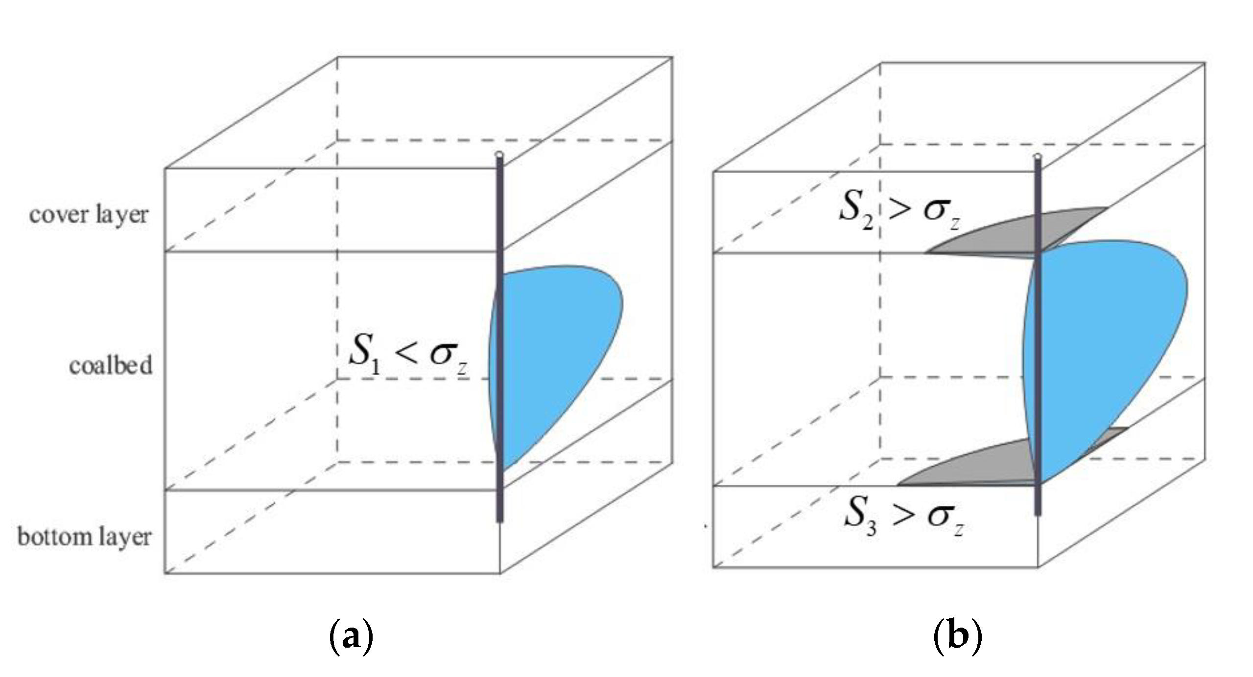
The hydraulic fracture starts from the coalbed. When the horizontal minimum principal stress of the fractured layer is less than the vertical stress, a vertical fracture is formed in the coalbed (Figure 1a).

(2)

Getting along with fracturing, the vertical fracture propagates longitudinally and break through the coal seam boundary. When the horizontal minimum principal stress of the cover and bottom layer is greater than the vertical stress, horizontal fractures are formed in the cover and bottom layer. Thus, an I-shaped fracture is produced (Figure 1b).

2.1. Fracture Propagation Simulation Model of Vertical Components

The vertical fracture propagation is shown in Figure 2. The fracture height is calculated according to the fracture height equation, which is not necessarily a parabola in most cases.

2.1.1. Continuity Equation

Before the vertical fracture propagates to the cover layer/bottom layer, the continuity equation is [35]

$$-\frac{\partial q_{\mathrm{V}}(x,t)}{\partial x}=\frac{2h(x,t)C_t(x,t)}{\sqrt{t-\tau (x)}}+\frac{\partial A(x,t)}{\partial t}$$

(1)

where A(x, t) is the cross-section area of fracture. C_t(x, t) is total fracturing fluid leak-off coefficient, m/min^0.5. τ(x) is the needed time of fracturing fluid to reach the given point x at time t, s.

When the vertical fracture propagates to the cover and bottom layer, the height of the vertical fracture formed by the fracturing treatment will not change, and then the continuity equation of the vertical fracture is

$$0=\frac{\partial q_{\mathrm{V}}(x,t)}{\partial x}+\frac{2H(x_0,t)C_t(x,t)}{\sqrt{t-\tau (x)}}+\frac{\partial A(x,t)}{\partial t}$$

(2)

where q_v is flow rate in vertical fracture, m³/s.

2.1.2. Pressure Drop Equations of the Vertical Component

According to the classic method of using pipe shape factor $\Phi (n^{\prime })$ in the pressure drop of fluid flowing in the parallel plate, pressure drop in 3D vertical fracture can be obtained:

$$\frac{\partial p_{\mathrm{V}}(x,t)}{\partial x}=-2^{n^{\prime }+1}{\left[\frac{(2n^{\prime }+1)q_{\mathrm{V}}(x,t)}{n^{\prime }\Phi (n^{\prime })h(x,t)}\right]}^{n^{\prime }}\frac{K^{\prime }}{d_{\mathrm{V}}{(x,0,t)}^{2n^{\prime }+1}}$$

(3)

$$\Phi (n^{\prime })={{\displaystyle {\int }_{-0.5}^{0.5}\left[\frac{d_{\mathrm{V}}(x,z,t)}{d_{\mathrm{V}}(x,0,t)}\right]}}^{\frac{2n\prime +1}{n\prime }}\mathrm{d}\left(\frac{z}{h(x,t)}\right)$$

(4)

where, p_V(x, t) is pressure inside vertical fracture at the given time t and point x, MPa. q_V(x, t) is flow rate in vertical fracture, m³/s. n′ is fracturing fluid flow behavior index, m/min^0.5. K′ is fracturing fluid consistency index, mPa⋅s^n′. h(x, t) is vertical fracture height, m. d_V(x, 0, t) is vertical fracture width at the center of cross section, m. t is fracturing time, s. The subscript “V” represents vertical fracture.

2.1.3. Fracture Width Equation of the Vertical Component

While fracture is propagating in coalbed, the net pressure in fracture (flowing pressure minus minimum horizontal principal stress) is

$$p(z)=p(x,t)-{\sigma }_{h1}-l\le z\le l$$

(5)

$$l=\frac{h(x,t)}{2}$$

(6)

where σ_h1 is least horizontal principal stress in coalbed, MPa.

At any height z, the width of the fracture width profile is [41]

$$d_{\mathrm{V}}(x,z,t)=\frac{4(1-{\nu }_1^2)}{E_1}\left[p(x,t)-{\sigma }_{h1}\right]\sqrt{l^2-z^2}-l\le z\le l$$

(7)

where ν₁ is Poisson’s ratio of coalbed, dimensionless. E₁ is Young’s modulus of coalbed, MPa.

When the vertical fracture propagates up and down to the cover/bottom layer, the net pressure (bottom-hole pressure minus the least horizontal principal stress) is

$$p(z)=\left\{\begin{array}{l}p(x,t)-{\sigma }_{h2} z_a \le z\le l\\ p(x,t)-{\sigma }_{h1} z_b\le z\le z_a\\ p(x,t)-{\sigma }_{h3} -l\le z\le z_b\end{array}\right.$$

(8)

$$z_a=\frac{H+h_{\mathrm{l}}(x,t)-h_{\mathrm{u}}(x,t)}{2}$$

(9)

$$z_b=-\frac{H+h_{\mathrm{l}}(x,t)-h_{\mathrm{u}}(x,t)}{2}$$

(10)

where σ_h2 is least horizontal principal stress of cover layer, MPa. σ_h3 is least horizontal principal stress of bottom layer, MPa. h₁(x, t) is the vertical fracture height in the bottom layer, m. h_u(x, t) is the vertical fracture height in cover layer, m. H is the thickness of coalbed, m.

According to the England and Green equation, the width of the fracture width profile at a specific height z is [38]

$$d_{\mathrm{V}}(x,z,t)=-16\frac{1-\nu {(z)}^2}{E(z)}{\displaystyle \underset{\left|z\right|}{\overset{l}{\int }}\frac{F(\tau )+zG(\tau )}{\sqrt{{\tau }^2-z^2}}\mathrm{d}\tau }$$

(11)

$$F(\tau )=-\frac{\tau }{2\pi }{\displaystyle \underset{0}{\overset{\tau }{\int }}\frac{f(z)}{\sqrt{{\tau }^2-z^2}}}dzG(\tau )$$

(12)

$$G(\tau )=-\frac{1}{2\pi \tau }{\displaystyle \underset{0}{\overset{\tau }{\int }}\frac{zg(z)}{\sqrt{{\tau }^2-z^2}}}dz$$

(13)

If the net pressure of vertical fracture is p_V(z) = f(z) + g(z), then the f(z) and g(z) are

$$f(z)=\frac{p_{\mathrm{V}}(z)+p_{\mathrm{V}}(-z)}{2}$$

(14)

$$g(z)=\frac{p_{\mathrm{V}}(z)-p_{\mathrm{V}}(-z)}{2}$$

(15)

2.1.4. Fracture Height Equation of Vertical Component

According to the theory of linear elastic fracture mechanics, when the vertical fracture is not propagated to the cover/bottom layer (h(x, t) < H), the stress intensity factors at ends up and down of fracture are mutually equal. Then, the fracture height is

$$K_{IC}=\frac{1}{\sqrt{\pi l}}{\displaystyle \underset{-l}{\overset{l}{\int }}p(z)\sqrt{\frac{l+z}{l-z}}dz}=[p(x,t)-{\sigma }_{h1}]\sqrt{\pi l}$$

(16)

When the vertical fracture extends to the cover layer and the bottom layer, the horizontal fracture initiates at the interface between the coal seam and the cover/bottom layer. Then, the fracture height is

$$h(x,t)=H$$

(17)

2.2. Model of Horizontal Component

2.2.1. Pressure Drop Equations of the Horizontal Component

When starting to produce horizontal fractures, the pressure drop also appears in them. During HF, the shape of horizontal fracture is circular. We can obtain the equation of pressure drop in upper and lower horizontal fracture as follows:

$$\frac{\mathrm{d}{p}_{\mathrm{upH}}(r)}{\mathrm{d}r}=-2{\left(\frac{q_{\mathrm{upH}}(r)}{\pi }\right)}^{n^{\prime }}{\left(\frac{2n^{\prime }+1}{n^{\prime }}\right)}^{n^{\prime }}\frac{K^{\prime }}{{\overline{d_{\mathrm{upH}}}}^{2n^{\prime }+1}}\frac{1}{r^{n^{\prime }}}$$

(18)

$$\frac{\mathrm{d}{p}_{\mathrm{lowH}}(r)}{\mathrm{d}r}=-2{\left(\frac{q_{\mathrm{lowH}}(r)}{\pi }\right)}^{n^{\prime }}{\left(\frac{2n^{\prime }+1}{n^{\prime }}\right)}^{n^{\prime }}\frac{K^{\prime }}{{\overline{d_{\mathrm{lowH}}}}^{2n^{\prime }+1}}\frac{1}{r^{n^{\prime }}}$$

(19)

where p_upH(r) is pressure inside upper horizontal fracture, MPa. p_lowH(r) is pressure inside lower horizontal fracture, MPa. q_upH(r) is flow rate in upper horizontal fracture, m³/s. q_lowH(r) is flow rate in lower horizontal fracture, m³/s. $\overline{d_{\mathrm{upH}}}$ is the average fracture width of upper horizontal fracture, m. $\overline{d_{\mathrm{lowH}}}$ is the average fracture width of lower horizontal fracture, m. The subscript “H” represents horizontal fracture.

2.2.2. Fracture Width Equation of the Horizontal Component

When the vertical fracture propagates up and down to the cover/bottom layer, horizontal fractures will be generated. A part of horizontal fractures will generate in the cover/bottom layer, the other part generates in the coalbed. According to Sneddon equation, the maximum width of horizontal fracture at r = r_w (r_w is wellbore radius) is

$$D_{\mathrm{H}\max }=\frac{8(1-{\nu }^2)}{\pi E}{\displaystyle \underset{0}{\overset{R}{\int }}\sigma (r){\cos }^{-1}(\frac{r}{R})\mathrm{d}r}$$

(20)

where σ(r) = p(r) − σ_h, D_Hmax is the maximum fracture width of horizontal fracture, m. r is radial coordinate of horizontal fracture, m. R is horizontal fracture radius at a given time, m.

Thus, the maximum width of upper and lower horizontal fractures between the coal seam and cover/bottom layer are represented respectively as

$$D_{\mathrm{up},\mathrm{H}\max }=D_{1,\mathrm{H}\max }+D_{2,\mathrm{H}\max }$$

(21)

$$D_{\mathrm{low},\mathrm{H}\max }=D_{1,\mathrm{H}\max }+D_{3,\mathrm{H}\max }$$

(22)

Therefore,

$$D_{\mathrm{up},\mathrm{H}\max }=\frac{8(1-{\nu }_1^2)}{\pi E_1}{\displaystyle \underset{0}{\overset{R_{\mathrm{up}}}{\int }}(p(x,t)-{\sigma }_{h1}){\cos }^{-1}(\frac{x}{R_{\mathrm{up}}})}\mathrm{d}x+\frac{8(1-{\nu }_2^2)}{\pi E_2}{\displaystyle \underset{0}{\overset{R_{\mathrm{up}}}{\int }}(p(x,t)-{\sigma }_{h2}){\cos }^{-1}(\frac{x}{R_{\mathrm{up}}})}\mathrm{d}x$$

(23)

$$D_{\mathrm{low},\mathrm{H}\max }=\frac{8(1-{\nu }_1^2)}{\pi E_1}{\displaystyle \underset{0}{\overset{R_{\mathrm{low}}}{\int }}(p(x,t)-{\sigma }_{h1}){\cos }^{-1}(\frac{x}{R_{\mathrm{low}}})}\mathrm{d}x+\frac{8(1-{\nu }_3^2)}{\pi E_3}{\displaystyle \underset{0}{\overset{R_{\mathrm{low}}}{\int }}(p(x,t)-{\sigma }_{h3}){\cos }^{-1}(\frac{x}{R_{\mathrm{low}}})}\mathrm{d}x$$

(24)

where R_up is upper horizontal fracture radius at a given time, m. R_low is lower horizontal fracture radius, m. ν_i (i = 1,2,3) is Poisson’s ratio, dimensionless. E_i (i = 1,2,3) is Young’s modulus, MPa. The subscript “1” represents coalbed, the subscript “2” represents cover layer, the subscript “3” represents bottom layer, the subscript “low” represents lower horizontal fracture, and the subscript “up” represents upper horizontal fracture.

2.3. Material Balance Equation

When the vertical fracture propagates to the cover/bottom layer, the flow rate was distributed to vertical fracture and generated horizontal fractures. Thus, the material balance equation is

$$Q=q_{\mathrm{upH}}+q_{\mathrm{lowH}}+2q_{\mathrm{V}}$$

(25)

where q_V is flow rate in vertical fracture, m³/s.

Meanwhile, the continuity equation of the vertical fracture and two horizontal fractures are

$$0=\frac{\partial q_{\mathrm{V}}(x,t)}{\partial x}+\frac{2H(x_0,t)C_t(x,t)}{\sqrt{t-\tau (x)}}+\frac{\partial A(x,t)}{\partial t}$$

(26)

$$q_{\mathrm{upH}}=\frac{8}{15}\pi (D_{\mathrm{up},\mathrm{H}\max }+\frac{R_{\mathrm{up}}}{2}\frac{{\mathrm{dD}}_{\mathrm{up},\mathrm{H}\max }}{\mathrm{d}{R}_{\mathrm{up}}})\frac{\mathrm{d}{R}_{\mathrm{up}}^2}{\mathrm{d}t}+2\pi {\displaystyle {\int }_0^t\frac{C(r)}{\sqrt{t-{\tau }^{\prime }}}}\frac{\mathrm{d}{R}_{\mathrm{up}}^2}{\mathrm{d}{\tau }^{\prime }}\mathrm{d}{\tau }^{\prime }$$

(27)

$$q_{\mathrm{lowH}}=\frac{8}{15}\pi (D_{\mathrm{low},\mathrm{H}\max }+\frac{R_{\mathrm{low}}}{2}\frac{\mathrm{d}{D}_{\mathrm{low},\mathrm{H}\max }}{\mathrm{d}{R}_{\mathrm{low}}})\frac{\mathrm{d}{R}_{\mathrm{low}}^2}{\mathrm{d}t}+2\pi {\displaystyle {\int }_0^t\frac{C(r)}{\sqrt{t-{\tau }^{\prime }}}}\frac{\mathrm{d}{R}_{\mathrm{low}}^2}{\mathrm{d}{\tau }^{\prime }}\mathrm{d}{\tau }^{\prime }$$

(28)

where C(r) is total fracturing fluid leak-off coefficient of horizontal fracture at x, m/s^0.5.

2.4. Boundary Conditions

In the ends of vertical fracture, the fracture height and flow rate are zero, and the pressure is the minimum horizontal principal stress of coalbed. At the ends of horizontal fractures, the pressure is the minimum horizontal principal stress of cover/bottom layer, respectively. In the propagating process of horizontal fractures, we can suppose as follows: (1) The fracturing fluid is assumed to fully saturate the fractures; (2) Within the propagation radius, the width of horizontal fractures is in accordance with parabola distribution; (3) Outside the propagation radius, the width is zero. Thus, the boundary conditions are

$$\left\{\begin{array}{l}{\left.q_{\mathrm{V}}(x,t)\right|}_{x=L_f}=0\\ {\left.p_{\mathrm{V}}(x,t)\right|}_{x=L_f}={\sigma }_{h1}\\ {\left.p_{\mathrm{H},\mathrm{up}}\right|}_{r=R_{\mathrm{up}}}={\sigma }_{h2}\\ {\left.p_{\mathrm{H},\mathrm{low}}\right|}_{r=R_{\mathrm{low}}}={\sigma }_{h3}\\ {\left.D_{\mathrm{H},\mathrm{up}}\right|}_{r=R_{\mathrm{up}}}=0\\ {\left.D_{\mathrm{H},\mathrm{low}}\right|}_{r=R_{\mathrm{low}}}=0\end{array}\right.$$

(29)

where L_f is half-length of fracture, m. R_up is radius of upper horizontal fracture, m. R_low is radius of lower horizontal fracture, m.

2.5. Initial Conditions

At the initial time, all parameters of vertical fracture are zero. The initial horizontal fracture radius is regarded as the wellbore radius because the horizontal fractures are calculated from the wellbore axis. Thus, the initial conditions are

$$\left\{\begin{array}{l}{\left.q_{\mathrm{V}}(0,t)\right|}_{t=0}=0\\ {\left.D_{\mathrm{V},\max }\right|}_{t=0}=0\\ {\left.D_{\mathrm{H},\max }\right|}_{t=\mathrm{T}}=0\\ {\left.R\right|}_{t=\mathrm{T}}=r_w\end{array}\right.$$

(30)

where T is the time of horizontal fracture began to propagating, s.

2.6. Coupling Conditions

According to the fracture propagation mechanism of I-shaped fracture, the vertical fracture and horizontal fractures are not completely independent. The pressure of two horizontal fractures and vertical fracture are equal in the intersection point. The total displacement pumped into wells equals to the sum of two horizontal fractures flow rate and vertical fracture flow rate. Hence, the coupling conditions are:

$$\left\{\begin{array}{l}{\left.p_{\mathrm{H},\mathrm{up}}\right|}_{r=0}={\left.p_{\mathrm{H},\mathrm{low}}\right|}_{r=0}={\left.p_{\mathrm{V}}\right|}_{x=0}\\ {\left.q_{\mathrm{H},\mathrm{up}}\right|}_{r=0}+{\left.q_{\mathrm{lowH}}\right|}_{r=0}+{\left.2q_{\mathrm{V}}\right|}_{x=0}=Q\end{array}\right.$$

(31)

where Q is total pumping displacement, m³/s.

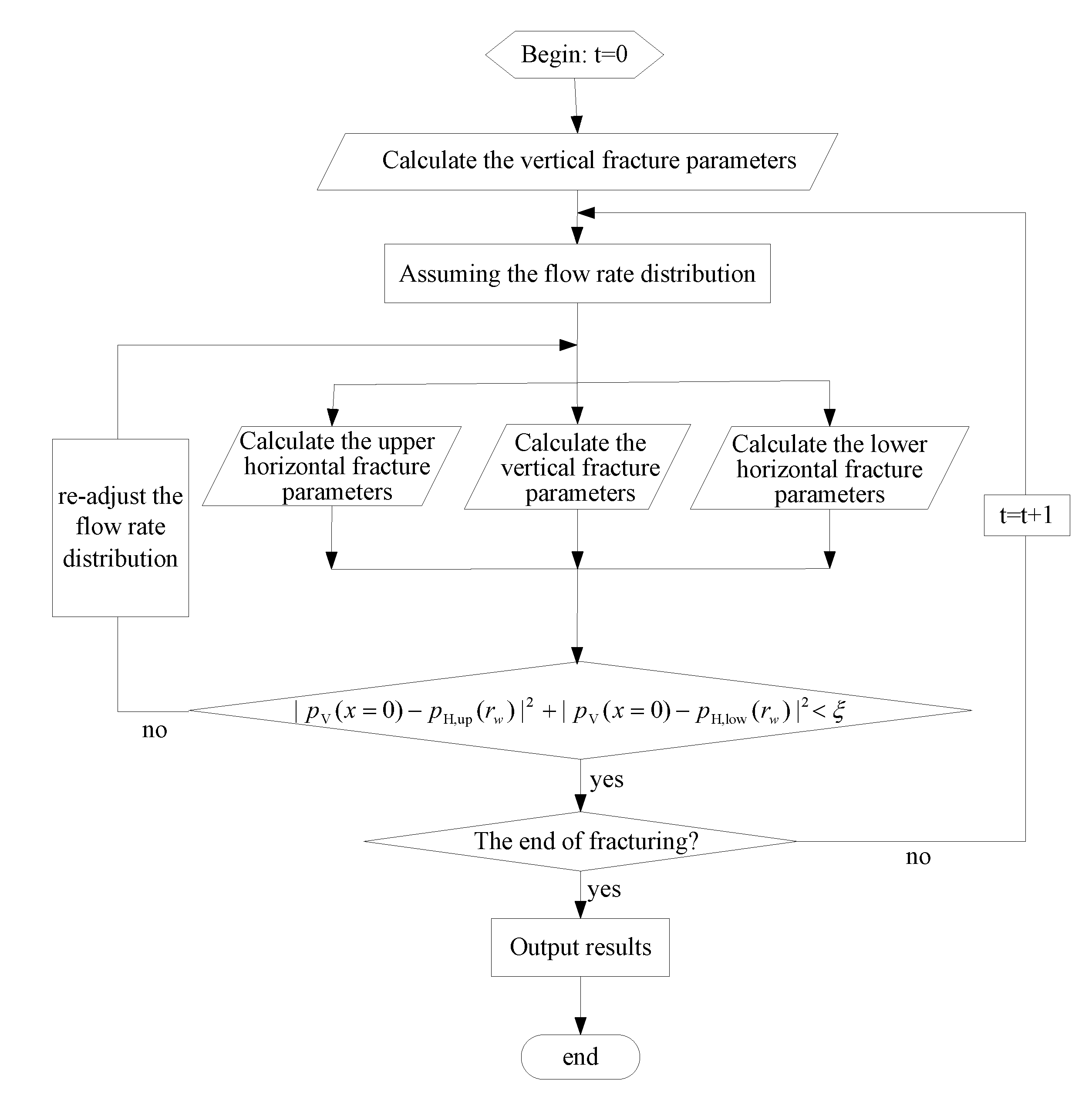
2.7. Numerical Method

The flow rate distribution of fracturing fluid is the key to solving the model. Once the flow rate ratio of horizontal fractures to vertical fracture is confirmed, the flow rate can be introduced into the horizontal and vertical fractures’ simulation models, respectively. According to the solution of the respective models, the geometric sizes of horizontal and vertical fractures can be obtained.

Figure 3 shows the flow chart of numerical method. The solving procedure of the above models involves five steps.

Step 1: Assume that the flow rate distribution in the initial moment is q_V: q_H,up: q_H,low = m₁: m₂: m₃;

Step 2: According to the flow rate distribution, the flow rates are substituted in vertical and horizontal fractures simulation models, respectively. At this time, according to solving steps of vertical and horizontal fracture simulation model, the bottom-hole pressures are calculated at the certain moment. The bottom-hole pressures of vertical fracture is p_V(x = 0), the bottom-hole pressures of upper horizontal fracture is p_H,up(r_w), and the bottom-hole pressure of lower horizontal fracture is p_H,low(r_w);

Step 3: Examine whether the bottom-hole pressures of two horizontal fractures are equal to the vertical fracture at the given moment. Generally, this is to determine whether the equation |p_V(x = 0) − p_H,up(r_w)|² + | p_V(x = 0) − p_H,up(r_w)|² < ξ (ξ is the maximum permissible error) is satisfied. If it is satisfied, the initial assumption of flow rate distribution is correct. Then, proceed to step 4. Otherwise, re-adjust the flow rate by the value of wellbore pressure and return to step 2;

Step 4: Calculate the bottom-hole pressures of the vertical and horizontal fractures at the next moment. Determine whether the fracturing ends. If it ends, proceed to step 5. Otherwise, return to step 3;

Step 5: The end.

3. PDA Model

The crustal stress of coalbed, cover layer, and bottom layer conforms to the distribution law of Figure 1. In this case, fracturing treatment will lead to the formation of I-shaped fracture, that is, the upper and lower horizontal fractures and a vertical fracture in the middle with symmetrical wings. In Section 2, the extension model of I-shaped fracture is established, and the following content is the establishment of PDA model of I-shaped fracture.

3.1. PDA Model of Vertical Fracture

At the time of t₁ and t, during the closure of the vertical fracture, according to the volume balance principle of the fluid, we can obtain the following equation [41]:

$$p_{w,\mathrm{V}}\left(t_1\right)-p_{w,\mathrm{V}}\left(t\right)=p_{\mathrm{V}}^{\ast }G\left(t_1,t\right)$$

(32)

$$p_{\mathrm{V}}^{\ast }=\frac{3}{2}\frac{E_1{C}_{\mathrm{V}}H\sqrt{t_{inj}}}{\left(1-{\nu }_1^2\right)H_w^2{\beta }_{\mathrm{V}}}$$

(33)

$$G\left(t_1,t\right)=\frac{4}{\pi }\left(g\left(t\right)-g\left(t_1\right)\right)$$

(34)

$$g\left(t\right)=\frac{2}{3}\left[{\left(1+t_D\right)}^{\frac{3}{2}}-t_D^{\frac{3}{2}}\right]+\frac{1}{2}\left[\left(1+t_D\right){\sin }^{-1}{\left(1+t_D\right)}^{-\frac{1}{2}}+t_D^{-\frac{1}{2}}\right]$$

(35)

$$t_D=\frac{t-t_{inj}}{t_{inj}}$$

(36)

where p_w,V(t) is bottom-hole pressure of vertical fracture at the given time t, MPa. $p_V^{*}$ is pseudo pressure of vertical fracture, MPa. H_w is vertical fracture height, m. β_V is the ratio of average pressure to bottom-hole pressure in vertical fracture. C_V is total fracturing fluid leak-off coefficient of vertical fracture, m/min^0.5. t_inj is the fracturing time, s.

For vertical fracture, the leak-off coefficient of post-fracturing fluid is

$$C_{\mathrm{V}}=\frac{2\left(1-{\nu }_1^2\right)H_w^2{\beta }_{\mathrm{V}}{p}_{\mathrm{V}}^{\ast }}{3E_{1}H\sqrt{t_{inj}}}$$

(37)

The maximum width of vertical fracture at the time of pump shutdown is

$$D_{\max ,\mathrm{V}}\left(t_{inj}\right)=\left\{\begin{array}{c}\frac{2\left(1-{\nu }_1^2\right)H_w}{E_1}\left(p_{ISI}-{\sigma }_{h1}\right), H_w<H\\ \frac{2\left(1-{\nu }_1^2\right)H_w}{E_1}\left(p_{ISI}-{\sigma }_{h1}\right)-\frac{4\left(1-{\nu }_1^2\right)H_w}{\pi E_1}\left({\sigma }_{h2}-{\sigma }_{h1}\right)\left({\cos }^{-1}\frac{H}{H_w}-\frac{H}{H_w}\ln \frac{H_w+\sqrt{H_w^2-H_{}^2}}{H}\right), H_w>H\end{array}\right.$$

(38)

where p_ISI is the instantaneous pressure of pump-stopping, MPa.

According to injection volume balance principle, at the time of stopping the pump, the fracture half-length is:

$$L_f=\frac{Q_{\mathrm{inj},\mathrm{V}}{t}_{inj}}{\frac{\pi }{3}{H}_w{D}_{\max ,\mathrm{V}}\left(t_{inj}\right){\beta }_{\mathrm{V}}+4C_{\mathrm{V}}H\sqrt{t_{inj}}g\left(t_{inj}\right)}$$

(39)

where Q_inj,V is the flow rate in vertical fracture during fracturing, m³/s.

The fracturing fluid efficiency is

$$\eta =\frac{\frac{\pi }{3}{L}_f{D}_{\max ,\mathrm{V}}\left(t_{inj}\right)H_w{\beta }_{\mathrm{V}}}{Q_{\mathrm{inj},\mathrm{V}}{t}_{inj}}$$

(40)

The time required for fracture closure is

$$g\left(t_c\right)=\frac{\pi D_{\max ,\mathrm{V}}\left(t_{inj}\right)H_w{\beta }_{\mathrm{V}}}{12C_{\mathrm{V}}H\sqrt{t_{inj}}}$$

(41)

3.2. PDA Model of Horizontal Fracture

According to the Carter filtration model and fracture propagation index, the of relationship between pressure fall-off and time is [42]

$$p_{w,\mathrm{Hup}}\left(t_1\right)-p_{w,\mathrm{Hup}}\left(t\right)=p_{\mathrm{Hup}}^{\ast }G\left(t_1,t\right)$$

(42)

$$p_{w,\mathrm{Hlow}}\left(t_1\right)-p_{w,\mathrm{Hlow}}\left(t\right)=p_{\mathrm{Hlow}}^{\ast }G\left(t_1,t\right)$$

(43)

$$p_{\mathrm{Hup}}^{\ast }=\frac{3{\pi }^2{C}_{\mathrm{Hup}}{f}_{p,\mathrm{up}}{E}_1\sqrt{t_{inj}}}{32(1-{\nu }_1^2){\beta }_{\mathrm{Hup}}}$$

(44)

$$p_{\mathrm{Hlow}}^{\ast }=\frac{3{\pi }^2{C}_{\mathrm{Hlow}}{f}_{p,\mathrm{low}}{E}_1\sqrt{t_{inj}}}{32(1-{\nu }_1^2){\beta }_{\mathrm{Hlow}}}$$

(45)

where p_w,Hup(t) is bottom-hole pressure of upper fracture, MPa. p_w,Hlow(t) is bottom-hole pressure of lower fracture, MPa. $p_{Hup}^{*}$ is pseudo pressure of upper horizontal fracture, MPa. In addition, $p_{Hlow}^{*}$ is pseudo pressure of lower horizontal fracture, MPa. C_Hup is total fracturing fluid leak-off coefficient of upper horizontal fracture, m/min^0.5. C_Hlow is total fracturing fluid leak-off coefficient of lower horizontal fracture, m/min^0.5. β_Hup is the ratio of average pressure to bottom-hole pressure in upper horizontal fracture, dimensionless. β_Hlow is the ratio of average pressure and bottom-hole pressure in lower horizontal fracture, dimensionless. f_p is the ratio of fracture leak-off area to fracture total area, dimensionless.

Based on the fracture leak-off coefficient which is fitted by the pseudo-pressure, some parameters of horizontal fracture are able to be obtained if the injection rate of fracture is known, such as leak-off coefficient of post-fracturing fluid, fracture radius and width, fracturing fluid efficiency and fracture closure time, etc.

The leak-off coefficient of post-fracturing fluid is

$$C_{\mathrm{Hup}}=\frac{32p_{\mathrm{Hup}}^{\ast }(1-{\nu }_1^2){\beta }_{\mathrm{Hup}}}{3{\pi }^2{f}_p{E}_1\sqrt{t_{inj}}}$$

(46)

$${\beta }_{\mathrm{Hup}}=3{\pi }^2/32$$

(47)

The fracturing fluid efficiency is:

$$\eta =\frac{\rho }{1+\rho }$$

(48)

$$\rho =\frac{p_{ISI}-p_c}{p_{\mathrm{Hup}}^{\ast }}\left\{\begin{array}{l}3\pi /16\\ 1/2\end{array}\right.$$

(49)

where p_c is fracture closure pressure, MPa.

At the stop time of fracturing, the fracture radius is

$$R_{p,\mathrm{up}}^3=\frac{3\eta Q_{\mathrm{inj},\mathrm{Hup}}{t}_{inj}{E}_1}{16\left(p_{ISI}-p_c\right)\left(1-{\nu }_1^2\right){\beta }_{\mathrm{Hup}}}$$

(50)

where Q_inj,Hup is the flow rate of upper horizontal fracture during fracturing treatment, m³/s.

At the stop time of fracturing, the average fracture width is

$${\overline{D}}_{\mathrm{Hup}}=\frac{16\left(1-{\nu }_1^2\right)\left(p_{ISI}-p_c\right)\beta R_{p,\mathrm{up}}}{3\pi E_1}$$

(51)

Similarly, the lower horizontal fracture parameters can be obtained.

3.3. Coupling Conditions

The pressures of two horizontal fractures are equal to the vertical fracture value at the bottom of the well. Thus, the pseudo pressures of two horizontal fractures are equal to the vertical fracture value. The total pumping displacement is equal to two horizontal fractures flow plus vertical fracture flow. Then, the coupling conditions are

$$\left\{\begin{array}{l}{p}_{\mathrm{V}}^{\ast }=p_{\mathrm{Hup}}^{\ast }=p_{\mathrm{Hlow}}^{\ast }\\ Q_{\mathrm{inj}}=Q_{\mathrm{inj},\mathrm{V}}+Q_{\mathrm{inj},\mathrm{Hup}}+Q_{\mathrm{inj},\mathrm{Hlow}}\end{array}\right.$$

(52)

By using the flow rate distribution principle and iterative method, we can obtain the leak-off coefficient of post-fracturing fluid, fracture length and width, fracturing fluid efficiency and fracture closure time of vertical fracture and the leak-off coefficient of post-fracturing fluid, fracture radius and width, and the fracturing fluid efficiency of upper and lower horizontal fracture. In addition, the numerical calculation method of PDA model for I-shaped fracture is similar to that in Section 2.7.

In the process of solving different practical problems, given an initial flow allocation, the iterative process will automatically narrow the interval containing the solution according to the judgment criteria, so that, after a certain number of iterations, a solution that meets the preset accuracy will be obtained.

3.4. History Matching of Pseudo Pressure

In order to obtain pseudo pressure, m points were selected in the period during shut-in and prior to closure, and an objective function is built as

$$J(p^{\ast })={\displaystyle \sum _{i=1}^m{\displaystyle \sum _{t_j\ge t_i}{\left[{\left(p_w\left(t_i\right)-p_w\left(t_j\right)\right)}^{obs}-{\left(p_w\left(t_i,p^{\ast }\right)-p_w\left(t_j,p^{\ast }\right)\right)}^{cal}\right]}^2}}$$

(53)

where (p_w(t_i) − p_w(t_j))^obs represents the observed pressure drop during time t_i to t_j, MPa. In addition, (p_w(t_i) − p_w(t_j))^cal represents the calculated pressure drop during time t_i to t_j, MPa. By adjusting pseudo pressure of p^*, the minimum error between observed pressure drop and calculated pressure drop can be obtained. Thus, this is an optimization model and can be expressed as

$$\min J(p^{*})$$

(54)

In this paper, the golden ration method was employed to solve the optimization model.

4. Results and Discussion

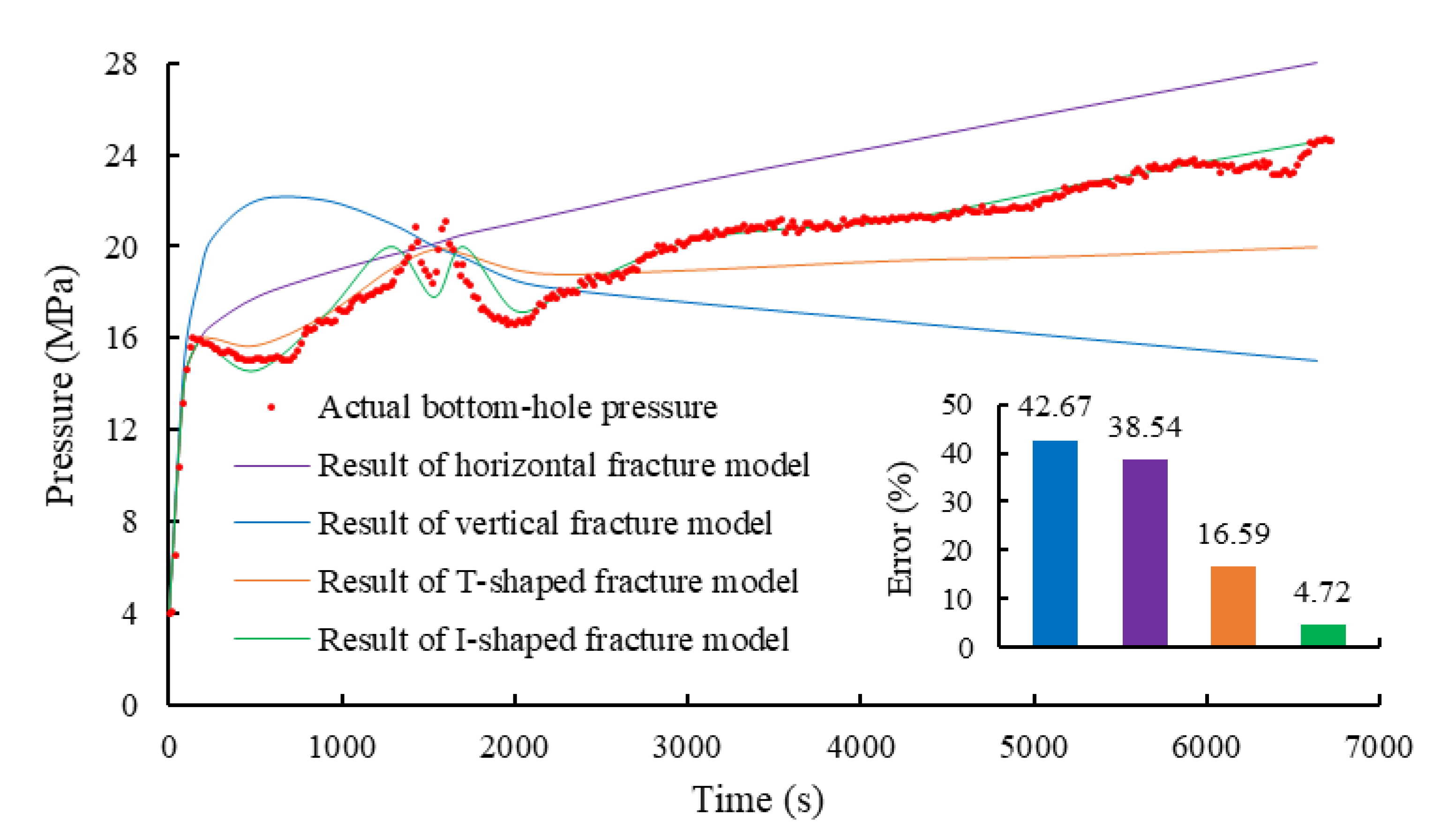
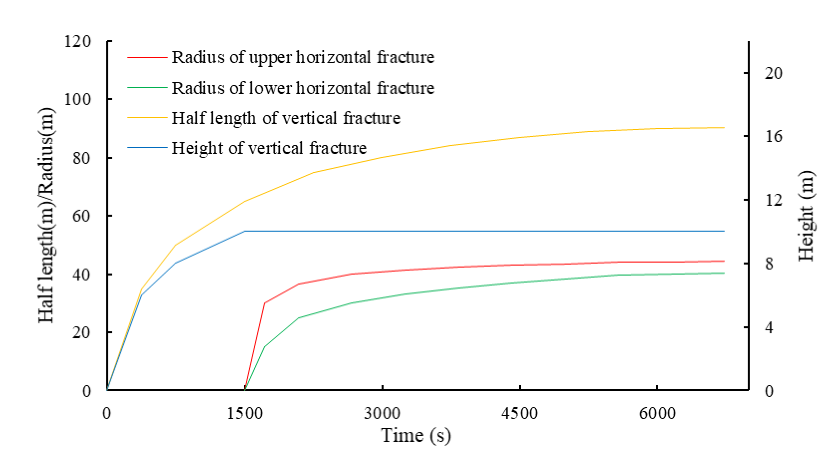
4.1. Results

The Hancheng area is a very important part in terms of the exploitation of CBM in China. Combining the I-shaped fracture propagation model with the PDA, a software on fracturing simulation has been applied in Hancheng area and achieved satisfactory effects.

Take well H-3-52 as an example.

Table 1. CBM formation properties and treatment parameters.

Parameter		Value	Parameter	Value
Young’s modulus (MPa)	Cover layer	18,000	Flow state index (dimensionless)	1
	Coalbed	3000	Fracturing fluid consistency coefficient (MPa·sn′)	1
	Bottom layer	15,000	Fracturing fluid density (kg/m3)	1000
Poisson ratio (dimensionless)	Cover layer	0.22	Fracturing fluid volume (m3)	469.3
	Coalbed	0.31	Injection rate (m3/min)	7
	Bottom layer	0.21	Coalbed permeability (10−3 μm2)	0.2
Coal seam thickness (m)		8.5	Coalbed porosity (dimensionless)	0.03

shows the formation properties and the treatment parameters that will be input into the simulation model. The construction curve of well H-3-52 is as shown in Figure 4. The values of all parameters in Table 1 are interpreted according to conventional logging data, as shown in Figure 5.

The construction curve of the well is shown in Figure 4. When fracturing treatment starts in the early stage, the fracture net pressure is less than the net overburden pressure. This phenomenon indicates that coalbed forms the vertical fracture. With the construction, the fracture net pressure began to exceed the net overburden pressure. This phenomenon indicates that formation forms the horizontal fractures. Therefore, the coalbed fracturing formed a complex fracture. Figure 5 shows the interpretation of rock mechanics parameters. In Figure 5, the difference between the minimum principal stress of cover/bottom layer and coalbed is 6 MPa. The minimum horizontal principal stress is the minimum stress in coal bed, and the overburden pressure is the minimum stress in cover/bottom layer. Thus, in Figure 4, the two labeled circle means that the horizontal fractures are formed.

Therefore, this paper simulates this fracturing treatment by the established models. Through continuous search and iteration, the ration of fractures flow rate for the propagation simulation model is: upper horizontal fracture: lower horizontal fracture: vertical fracture = 0.2376:0.2563:0.5061. We also simulate this treatment with a vertical fracture propagation model, a vertical fracture propagation model, and a T-shaped fracture propagation model. Figure 6 shows the bottom-hole pressure match using an I-shaped fracture propagation model, vertical fracture model, horizontal fracture model, and T-shaped fracture model. As seen in Figure 6, only the simulated pressure of I-shaped fracture model is consistent with the actual pressure on site (the error is 4.72%). The T-shaped fracture model deviates greatly from the actual situation in pressure simulation (the error is 16.59%). The pressure errors calculated by the conventional vertical and horizontal fracture models are completely distorted, and both of the trend and shape are different from the actual value.

Then, we set the above ration as the initial ration of PDA. Through continuous search and iteration, the ration of the fracture flow rate for the PDA model is: upper horizontal fracture: lower horizontal fracture: vertical fracture = 0.2503:0.2588:0.4909. In addition, we also analyzed the phase of pressure fall-off with T-shaped fracture PDA and convention PDA. Figure 7 shows the bottom-hole pressure match using I-shaped fracture PDA, T-shaped fracture PDA, and convention vertical and horizontal fracture PDA. As seen in Figure 7, an accurate pressure history match is obtained using a new model. However, the T-shaped fracture model and convention models cannot obtain the satisfactory pressure history match because of the inappropriate fracture shape.

The changes of fracture parameters during fracturing treatment are shown in Figure 8. In addition, the calculation of geometric sizes using a new model is shown in

Table 2. The calculation results of fracture geometry.

	Upper Horizontal Fracture Geometry		Lower Horizontal Fracture Geometry		Vertical Fracture Geometry
	Width (mm)	Radius (m)	Width (mm)	Radius (m)	Width (mm)	Half Length (m)	Height (m)
I-shaped Fracture propagation model	5.1589	40.4279	5.3013	44.3198	6.7478	90.1286	15
PDA	5.0461	42.2461	5.1387	43.4789	6.2365	84.2353

. As seen from the table, the simulation results of the propagation model and PDA have a slight difference. Meanwhile, based on the PDA model, the fracturing fluid efficiency is 14.9%, the leak-off coefficient of post-fracturing fluid is 0.001206 m/min^0.5, and the fracture closure time is 19.62 min.

The model proposed in this paper has good universality and is applicable to different geological conditions and rock types. Taking the construction data and logging data of well H-3-52 in the Hancheng area as an example, compared with the T-shaped fracture model and the conventional fracture models, the numerical simulation results of the I-shaped fracture model established in this paper are more accurate, and are in good agreement with the results of PDA model, which has been compared and analyzed in detail before.

For the fracture model and PDA model proposed in this paper, it is one of the further research directions to adopt a more complex iterative algorithm as an alternative to the numerical simulation method. In general, the I-shaped fracture model and PDA model established in this paper can provide effective guidance for simulating fracture initiation/propagation and pressure decline.

4.2. Discussion

4.2.1. Influence of Crustal Stress Variation on Fracture Geometry

In order to study the variation law of I-shaped fracture geometry with crustal stress, under the condition that the stress state meets the formation conditions of I-shaped fracture, take two points respectively around the minimum principal stress of the cover and bottom layer of well H-3-52 in 1 MPa steps, and calculate the variation of I-shaped fracture geometry. The specific results are shown in

Table 3. Fracture geometry changes with crustal stress of cover layer.

Parameter	Value
Crustal stress of cover layer (MPa)	17.7	18.7	19.7	20.7	21.7
Upper horizontal fracture radius (m)	44.8345	43.2174	40.4279	37.9618	36.3447
Vertical fracture half length (m)	80.3046	83.9097	90.1286	95.6264	99.2316
Lower horizontal fracture radius (m)	39.4889	41.2617	44.3198	47.0233	48.7961

and

Table 4. Fracture geometry changes with crustal stress of bottom layer.

Parameter	Value
Crustal stress of bottom layer (MPa)	18.4	19.4	20.4	21.4	22.4
Upper horizontal fracture radius (m)	36.4255	37.6384	40.4279	42.8940	44.5111
Vertical fracture half length (m)	81.2059	84.6308	90.1286	96.3475	99.0513
Lower horizontal fracture radius (m)	49.1507	47.3779	44.3198	41.6163	39.9321

.

In the above discussion, the horizontal minimum principal stress of the coal seam is less than the vertical stress, and the horizontal minimum principal stress of the cover and bottom layer is greater than the vertical stress. Therefore, these changes in these values can lead to the formation of I-shaped fracture.

It can be seen from Table 3 that, with crustal stress of cover layer increasing, the upper horizontal joint radius gradually decreases, and the half length of vertical fracture and the lower horizontal joint radius gradually increase. Similarly, with crustal stress of bottom layer increasing, the lower horizontal fracture radius gradually decreases, and the half length of vertical fracture and the upper horizontal fracture radius gradually increases. Compared with the horizontal fracture radius of cover and bottom layer, the change of crustal stress has a more significant impact on the half length of vertical fracture.

4.2.2. Influence of Fracturing Fluid on Fracture Geometry

The flow index is 1 and remains unchanged. First, the influence of fracturing fluid consistency coefficient K′ on fracture geometry is discussed. K′ gradually increases to 5 MPa·s^n′ in steps of 1 MPa·s^n′. The simulated geometric results of I-shaped fracture are shown in

Table 5. Fracture geometry changes with a fracturing fluid consistency coefficient.

Parameter	Value
Fracturing fluid consistency coefficient (MPa·sn’)	1	2	3	4	5
Upper horizontal fracture radius (m)	40.4279	42.3280	43.4196	44.4303	45.3197
Vertical fracture half length (m)	90.1286	94.3646	96.7981	99.0513	101.0342
Lower horizontal fracture radius (m)	44.3198	46.4028	47.5995	48.7075	49.6825

.

The higher the fracturing fluid consistency coefficient is, the smaller the fracture height will be, which will cause the fracture to propagate further. It can be seen from Table 5 that, with the increase of the fracturing fluid consistency coefficient, the radius of the horizontal fractures in the cover and bottom layers and the half length of the vertical fracture gradually increase. The simulation results are consistent with the actual situation.

Table 6. Fracture geometry changes with leak-off coefficient of post-fracturing fluid.

Parameter	Value
Leak-off coefficient of post-fracturing fluid (m/min0.5)	0.00100098	0.0010854	0.001206	0.001327	0.001447
Upper horizontal fracture radius (m)	41.9642	41.1152	40.4279	39.6193	38.8108
Vertical fracture half length (m)	93.5535	91.6608	90.1286	88.3260	86.5235
Lower horizontal fracture radius (m)	46.0040	45.0732	44.3198	43.4334	42.5470

shows the results of the change of I-shaped fracture geometry with the leak-off coefficient post-fracturing fluid. It can be seen from Table 6 that, with the increase of leak-off coefficient, the radius of horizontal fractures in the cover and bottom layers gradually decreases, while the half length of vertical fracture also gradually decreases. The greater the filtration is, the greater the limitation of I-shaped fracture propagation will be.

5. Conclusions

The I-shaped fracture model and PDA model proposed in this paper are effective tools to simulate the hydraulic fractures. The effectiveness of the methods is analyzed through examples, and the following conclusions can be summarized.

(1)

The adequate research regarding the fracture propagation mechanism is essential for coal seam fracturing. The I-shaped fracture is often occurred in coal seam fracturing. This paper elaborates its propagation mechanism.

(2)

This paper developed the 3D propagation simulation model of I-shaped fracture. Pressure-drop equations of fluid flowing in fractures, fracture width equation, fracture height equation, and continuity equation of fluid flowing in fractures are developed based on the 3D fracture propagation model. Furthermore, the coupling conditions of vertical fracture and horizontal fractures are established based on the flow rate distribution and the bottom-hole pressure equality. Moreover, a satisfactory numerical method of 3D model is developed based on the iterative method. Then, we can obtain the fracture geometries and total fracturing fluid leak-off coefficient.

(3)

This paper developed the PDA model of an I-shaped fracture. The coupling conditions and numerical method are similar to a P3D propagation simulation model. Then, we can obtain the leak-off coefficient of post-fracturing fluid, fracture geometries, fracturing fluid efficiency, and fracture closure time, etc.

(4)

The proposed models have been applied to a realistic CBM well of the Hancheng area. We obtained the fracture geometries, fracturing fluid efficiency, etc. It is concluded that the established two models are effective tools for the simulation of fracture initiation/propagation and pressure decline of post-fracturing.

References

1. Guo, Z.; Chen, Y.; Zhou, X.; Zeng, F. Inversing fracture parameters using early-time production data for fractured wells. Inverse Probl. Sci. Eng. 2020, 28, 674–694. [Google Scholar] [CrossRef]
2. Adachi, J.; Siebrits, E.; Peirce, A.; Desroches, J. Computer simulation of hydraulic fractures. Int. J. Rock Mech. Min. Sci. 2007, 44, 739–757. [Google Scholar] [CrossRef]
3. Guo, Z.; Zhao, J.; You, Z.; Li, Y.; Zhang, S.; Chen, Y. Prediction of coalbed methane production based on deep learning. Energy 2021, 230, 120847. [Google Scholar] [CrossRef]
4. Wang, D.; You, Z.; Johnson, R.L.; Wu, L.; Bedrikovetsky, P.; Aminossadati, S.M.; Leonardi, C. Numerical investigation of the effects of proppant embedment on fracture permeability and well production in Queensland coal seam gas reservoirs. Int. J. Coal Geol. 2021, 242, 103689. [Google Scholar] [CrossRef]
5. Wang, T.; Zhou, W.; Chen, J.; Xiao, X.; Li, Y.; Zhao, X. Simulation of hydraulic fracturing using particle flow method and application in a coal mine. Int. J. Coal Geol. 2014, 121, 1–13. [Google Scholar] [CrossRef]
6. Guo, Z.; Zhao, J.; Sun, X.; Wang, C.; Guo, D.; Hu, H.; Wang, H.; Zeng, Q. A Novel Continuous Fracture Network Model: Formation Mechanism, Numerical Simulation and Field Application. Geofluids 2022, 2022, 1468–8115. [Google Scholar] [CrossRef]
7. Feng, Q.; Wu, C.F.; Lei, B. Coal/Rock mechanics features of Qinshui basin and fracturing crack control. Coal Sci. Technol. 2011, 39, 100–103. [Google Scholar]
8. Cheng, Y.F.; Wu, B.L.; Dong, B.X.; Li, L.D.; Huang, H.Y. Establishment and application of “T” shape fracture propagation model in hydraulic fracturing of methane well. J. China Coal Soc. 2013, 38, 1430–1434. [Google Scholar]
9. Wu, X.; Xi, C.; Wang, G. The mathematic model research of complicated fractures system in coalbed methane wells. Nat. Gas Ind. 2006, 26, 124–126. [Google Scholar]
10. Zhang, Z.; Qin, Y.; Yi, T.; You, Z.; Yang, Z. Pore Structure Characteristics of Coal and Their Geological Controlling Factors in Eastern Yunnan and Western Guizhou, China. ACS Omega 2020, 5, 19565–19578. [Google Scholar] [CrossRef]
11. Zhang, Z.; Qin, Y.; Wang, G.; Sun, H.; You, Z.; Jin, J.; Yang, Z. Evaluation of Coal Body Structures and Their Distributions by Geophysical Logging Methods: Case Study in the Laochang Block, Eastern Yunnan, China. Nat. Resour. Res. 2021, 30, 2225–2239. [Google Scholar] [CrossRef]
12. Guo, Z.; Chen, Y.; Yao, S.; Zhang, Q.; Liu, Y.; Zeng, F. Feasibility Analysis and Optimal Design of Acidizing of Coalbed Methane Wells. J. Energy Resour. Technol. 2019, 141, 082906. [Google Scholar] [CrossRef] [Green Version]
13. Guo, D.-L.; Ji, L.-J.; Zhao, J.-Z.; Liu, C.-Q. 3-D Fracture Propagation Simulation and Production Prediction in Coalbed. Appl. Math. Mech. 2001, 22, 385–393. [Google Scholar] [CrossRef]
14. Tang, S.; Zhu, B.; Yang, Z. Effect of crustal stress on hydraulic fracturing in coalbed methane wells. J. China Coal Soc. 2011, 36, 65–69. [Google Scholar]
15. Garikapati, H.; Verhoosel, C.V.; van Brummelen, E.H.; Zlotnik, S.; Díez, P. Sampling-based stochastic analysis of the PKN model for hydraulic fracturing. Comput. Geosci. 2019, 23, 81–105. [Google Scholar] [CrossRef] [Green Version]
16. Liu, Y.; Wang, C.; Zhou, H. Optimization scheme of hydraulic fracturing simulation experiments using mixed-level uniform design method based on the PKN model. J. Phys. Conf. Ser. 2020, 1574, 012165. [Google Scholar] [CrossRef]
17. Golovin, S.; Isaev, V.; Baykin, A.; Kuznetsov, D.; Mamontov, A. Hydraulic fracture numerical model free of explicit tip tracking. Int. J. Rock Mech. Min. Sci. 2015, 76, 174–181. [Google Scholar] [CrossRef]
18. Nguyen, H.T.; Lee, J.H.; Elraies, K.A. A review of PKN-type modeling of hydraulic fractures. J. Pet. Sci. Eng. 2020, 195, 107607. [Google Scholar] [CrossRef]
19. Wrobel, M. On the application of simplified rheological models of fluid in the hydraulic fracture problems. Int. J. Eng. Sci. 2020, 150, 103275. [Google Scholar] [CrossRef]
20. Gu, M.; Mohanty, K. Effect of foam quality on effectiveness of hydraulic fracturing in shales. Int. J. Rock Mech. Min. Sci. 2014, 70, 273–285. [Google Scholar] [CrossRef]
21. Zia, H.; Lecampion, B.; Zhang, W. Impact of the anisotropy of fracture toughness on the propagation of planar 3D hydraulic fracture. Int. J. Fract. 2018, 211, 103–123. [Google Scholar] [CrossRef]
22. Baykin, A.N.; Golovin, S.V. Application of the Fully Coupled Planar 3D Poroelastic Hydraulic Fracturing Model to the Analysis of the Permeability Contrast Impact on Fracture Propagation. Rock Mech. Rock Eng. 2018, 51, 3205–3217. [Google Scholar] [CrossRef]
23. Redhaounia, B.; Bédir, M.; Gabtni, H.; Batobo, O.I.; Dhaoui, M.; Chabaane, A.; Khomsi, S. Hydro-geophysical characterization for groundwater resources potential of fractured limestone reservoirs in Amdoun Monts (North-western Tunisia). J. Appl. Geophys. 2016, 128, 150–162. [Google Scholar] [CrossRef]
24. Dontsov, E.; Peirce, A. An enhanced pseudo-3D model for hydraulic fracturing accounting for viscous height growth, non-local elasticity, and lateral toughness. Eng. Fract. Mech. 2015, 142, 116–139. [Google Scholar] [CrossRef] [Green Version]
25. Zhang, X.; Wu, B.; Jeffrey, R.G.; Connell, L.D.; Zhang, G. A pseudo-3D model for hydraulic fracture growth in a layered rock. Int. J. Solids Struct. 2017, 115-116, 208–223. [Google Scholar] [CrossRef]
26. Zia, H.; Lecampion, B. PyFrac: A planar 3D hydraulic fracture simulator. Comput. Phys. Commun. 2020, 255, 107368. [Google Scholar] [CrossRef]
27. Skopintsev, A.; Dontsov, E.; Kovtunenko, P.; Baykin, A.; Golovin, S. The coupling of an enhanced pseudo-3D model for hydraulic fracturing with a proppant transport model. Eng. Fract. Mech. 2020, 236, 107177. [Google Scholar] [CrossRef]
28. Linkov, A.; Markov, N. Improved pseudo three-dimensional model for hydraulic fractures under stress contrast. Int. J. Rock Mech. Min. Sci. 2020, 130, 104316. [Google Scholar] [CrossRef]
29. Wen, M.; Huang, H.; Hou, Z.; Wang, F.; Qiu, H.; Ma, N.; Zhou, S. Numerical simulation of the non-Newtonian fracturing fluid influences on the fracture propagation. Energy Sci. Eng. 2022, 10, 404–413. [Google Scholar] [CrossRef]
30. Peirce, A.; Detournay, E. An implicit level set method for modeling hydraulically driven fractures. Comput. Methods Appl. Mech. Eng. 2008, 197, 2858–2885. [Google Scholar] [CrossRef]
31. Salimzadeh, S.; Paluszny, A.; Zimmerman, R. Three-dimensional poroelastic effects during hydraulic fracturing in permeable rocks. Int. J. Solids Struct. 2017, 108, 153–163. [Google Scholar] [CrossRef]
32. Karimi-Fard, M.; Firoozabadi, A. Numerical Simulation of Water Injection in Fractured Media Using the Discrete-Fracture Model and the Galerkin Method. SPE Reserv. Eval. Eng. 2003, 6, 117–126. [Google Scholar] [CrossRef]
33. Hossain, M.; Rahman, M. Numerical simulation of complex fracture growth during tight reservoir stimulation by hydraulic fracturing. J. Pet. Sci. Eng. 2008, 60, 86–104. [Google Scholar] [CrossRef]
34. Chen, E.; Leung, C.K.; Tang, S.; Lu, C. Displacement discontinuity method for cohesive crack propagation. Eng. Fract. Mech. 2018, 190, 319–330. [Google Scholar] [CrossRef]
35. Zvyagin, A.V.; Luzhin, A.A.; Panfilov, D.I.; Shamina, A.A. Numerical method of discontinuous displacements in spatial problems of fracture mechanics. Mech. Solids 2021, 56, 119–130. [Google Scholar] [CrossRef]
36. Kim, H.; Onishi, T.; Chen, H.; Datta-Gupta, A. Parameterization of embedded discrete fracture models (EDFM) for efficient history matching of fractured reservoirs. J. Pet. Sci. Eng. 2021, 204, 108681. [Google Scholar] [CrossRef]
37. Guo, Z.; Zhao, J.; Li, Y.; Zhao, Y.; Hu, H. Theoretical and experimental determination of proppant-crushing ratio and fracture conductivity with different particle sizes. Energy Sci. Eng. 2022, 10, 177–193. [Google Scholar] [CrossRef]
38. Guo, D.; Zhao, J.; Guo, J.; Zeng, X. Three-dimensional model and mathematical fitting method of pressure test data after fracturing. Nat. Gas Ind. 2001, 21, 49–52. [Google Scholar]
39. Guo, D.; Wu, G.; Liu, X.; Zhao, J. Analyzing method of pressure decline to identify fracture parameters. Nat. Gas Ind. 2003, 23, 83–85. [Google Scholar]
40. Zhao, W.; Ji, G.; Li, K.; Liu, W.; Xiong, L.; Xiao, J. A new pseudo 3D hydraulic fracture propagation model for sandstone reservoirs considering fracture penetrating height. Eng. Fract. Mech. 2022, 264, 108358. [Google Scholar] [CrossRef]
41. Ji, L.; Guo, D.; Zhao, J.; Wu, G. 3-D models and its computation of acid fracture simulation. Drill. Prod. Technol. 2000, 23, 39–43. [Google Scholar]
42. Guo, D.; Zhang, S.; Li, T.; Pu, X.; Zhao, Y.; Ma, B. Mechanical mechanisms of T-shaped fractures, including pressure decline and simulated 3D models of fracture propagation. J. Nat. Gas Sci. Eng. 2018, 50, 1–10. [Google Scholar] [CrossRef]
Figure 1. (a) shows the vertical component of I-shaped fracture which formed firstly due to the minimum principal stress being the minimum horizontal principal stress, and (b) shows the horizontal component of I-shaped fracture which formed firstly due to the minimum principal stress being the minimum horizontal principal stress in both cover and bottom layers. S2 and S3 are usually greater than S1, while there is little difference between S2 and S3.
Energies 15 05811 g001
Figure 2. Schematic of vertical fracture propagation.
Energies 15 05811 g002
Figure 3. The flow chart of the numerical method.
Energies 15 05811 g003
Figure 4. The construction curve of the well.
Energies 15 05811 g004
Figure 5. The interpretation data of rock mechanics parameters.
Energies 15 05811 g005
Figure 6. Comparison of bottom-hole pressure calculated by different models during fracturing treatment.
Energies 15 05811 g006
Figure 7. Comparison of bottom-hole pressure calculated by different models at the phase of pressure fall-off.
Energies 15 05811 g007
Figure 8. Variation diagram of fracture parameters during fracturing treatment.
Energies 15 05811 g008