Laser Profilometry on Micro-PTC

Abstract

Profilometry is useful in detecting surface faults on solar concentrators, which can be imperfectly manufactured, thus affecting system performance. Profilometric analyses are performed on a micro-parabolic trough collector (m-PTC), with reduced sizes and greater mirror curvature than a usual PTC. The peculiar dimensions and shape of this micro-PTC request to develop a specific configuration of laser profilometry. It includes a laser diode with a converging lens placed in front of it, ensuring that the mirror curvature does not affect the beam reflection. A new method to calculate the spot position furnishes the reflected beam center even if it lies outside the target, giving it a virtual expansion. The profile is assessed with an iterative calculation, starting from a first point, physically measured. The results are the 3D profile reconstruction of the parabolic mirror and a map of the slope error for each mirror point. It also estimates the intercept factor, a parameter fundamental to optimize the m-PTC system, whose value is in agreement with a structured light measurement on the same object. This intercept factor was obtained averaging the local intercept factor calculated for each mirror point, which individuates the mirror portions not focusing the sunrays on the tube.

1. Introduction

Systems based on the concentration of solar radiation represent a well-established sector in the framework of renewable energy technologies. The principal components are the reflectors coupled to a receiver, exploiting various geometries. Parabolic trough collector (PTC) systems have a linear parabolic reflector that concentrates the solar irradiance over a linear absorber and the irradiance distribution depends on the geometric features of the mirror surface. Since the working principle of PTC is based on the mirror parabolic profile, the optical quality of the collector surface is a crucial aspect to be controlled in order to optimize the sunlight collection. The aim is to maximize the irradiation uniformity over the trough absorber; an incorrect parabolic curvature of the mirror or a localized defect on the mirror surface can direct sunlight outside the absorber. The sensitivity to these imperfections of the trough collector surface increases as the diameter of the linear receiver decreases.

For the production of heat at a medium temperature, 150–250 °C, solar collectors could be smaller with respect to the usual PTCs employed in the large high-temperature plants [1,2,3,4]. The advantage of having reduced dimensions permits to install these solar collection systems in small areas or even on building roofs [5,6,7,8]. The examined micro-PTC (m-PTC) is ten times smaller than a common PTC. Experimentations on this m-PTC are aimed to verify the dimension scalability of the PTC technology. The advantage would be to produce electricity and thermal energy near the end user in industrial and residential contexts.

There are various strategies to assess the single profile of a linear mirror or to detect the total shape of a reflector. Optical profilometry is suitable to check parabolic trough collectors; more generally, techniques of geometrical optics [9,10,11] can be applied to PTC mirrors. The most common optical techniques used on PTCs are: laser scanning profilometry, photogrammetry, and others based on image processing analysis, such as tube reflection analysis and deflectometry.

The principle of the laser scanning technique is based on the fact that for each luminous ray impinging on a point of the examined mirror surface, the reflected ray is deviated in agreement with the value of the local surface slope; if this slope value is correct, the beam will be reflected toward the parabola focus.

Optical profilometers based on point-by-point detection, such as in [12,13,14] for the characterization of PTC concentrators are more precise, so they are quite time consuming because they need to scan the whole mirror. Since the measurement time depends on the mirror surface dimensions and increases as the requested resolution improves, this method is advisable for small mirrors.

Photogrammetry [15,16], which is essentially the interpretation of photographic images, can be a powerful tool for the geometrical analysis of collectors and solar components. The setup requires applying a grid of targets that the camera can automatically detect on the surface to be measured.

Other methods are based on the analysis of the tube image reflected by the collector under test. One advantage is rapidity, because they can examine, in an acceptably short time, the total PTC surface.

If the observation distance exceeds the mirror focal distance, the image visible from far away covers the whole collector and the observer sees a uniformly colored image.

In general, collector surface defects subtract information from the image in the defective points, which appear as zones of altered intensity inside the image; several authors have successfully applied these detections to the PTCs [17,18,19].

A more empirical approach is to use calibrated masks [20,21]. In this case, the collector under examination reproduces the image of the mask and this image is suitably elaborated to extract the surface quality data.

Another powerful tool for the study of the optical quality of PTC is called deflectometry. It is a technique that utilizes the deformation and displacement of a sample pattern after reflection from a test surface to infer the surface [22,23]. A regular fringe pattern is displayed on a monitor and the tested object reflects it toward the camera. Any irregularities in the object give rise to a distortion of the observed fringes, which can be evaluated quantitatively. Fringe reflection can be also considered to assess surface quality on heliostats or solar mirrors [24,25]; these methods can provide a global reconstruction and a detailed characterization of the curve concentrator. The information about local slope errors is already interesting and useful for a surface quality assessment, but a suitable elaboration of the acquired image can provide a 3D reconstruction of the total collector surface. The 3D reconstruction of the collector gives a visual, comprehensive, and immediate overview of the quality of the reflecting surface [26].

During the past decades, the Solar Collector Laboratory of CNR-INO has studied [27] and experimented [28] several optical techniques that employ this approach to assess the surface quality on solar mirrors. A method based on color-coded patterns was applied to deformable heliostats [26], reconstructing the shape of the reflecting surface. This image processing technique is based on the projection of a luminous pattern composed of colored points over the heliostat. A suitable elaboration separating the different colors extracts the geometrical parameters and provides a reconstruction of the entire mirror. Another method that was applied to a PTC [29] examines, from a far point, the receiver image created by the collector. This optical configuration corresponds to observing an object, the receiver, through an optical system, the collector, in magnification conditions.

The exact fabrication of the parabolic profile is essential for the correct working of the PTC. Unfortunately, even small errors in the surface manufacture can cause significant energy losses in the solar collection system. A dedicated experimentation was carried out to develop a procedure practically applicable to PTC with reduced dimensions with respect to the typical ones.

A new prototype of micro-PTC was optically designed, realized, and tested [30,31,32,33]. The micro-PTC was successively utilized for the realization of a concentrated solar power plant. Solar energy could play an important role, especially in urban areas for residential or industrial applications. The thermal energy for residential application is a relevant part of the entire demand, so solar technologies could have a significant role in reducing fossil fuel consumption. In particular, it is important to realize systems of reduced dimension that allow the installation of CSP systems also in domestic environments.

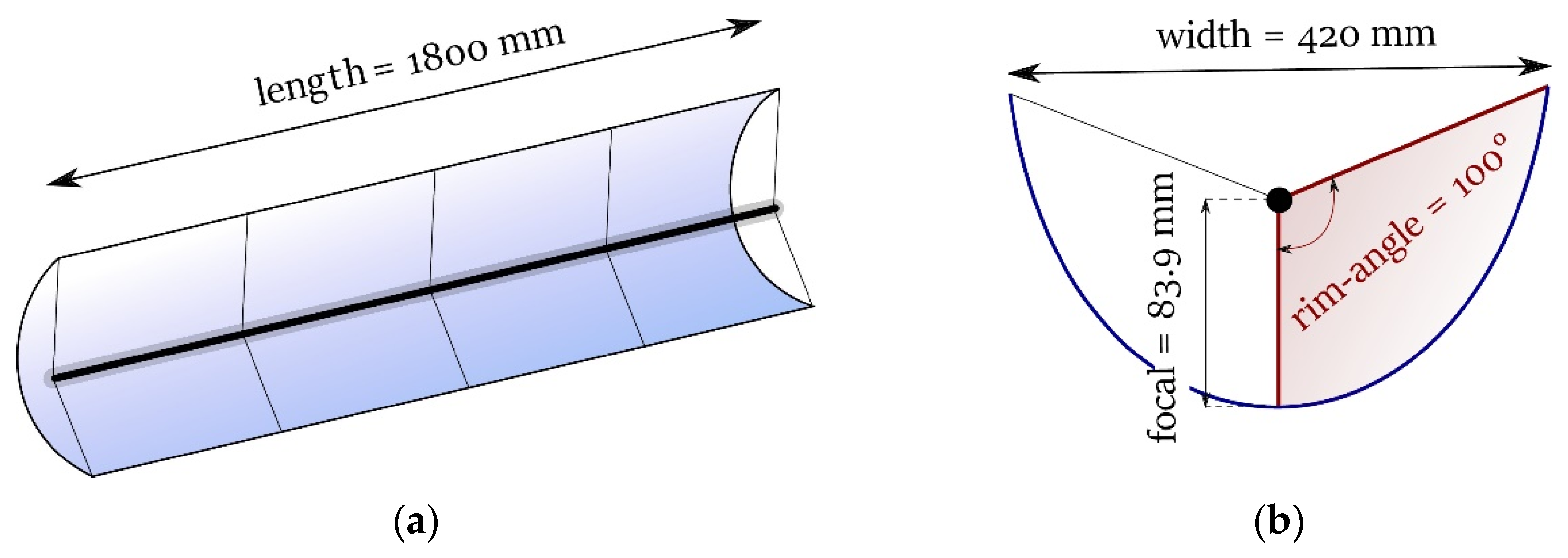
The m-PTC has 1800 mm of length, 420 mm of collector aperture, 83.9 mm of focal length, and 100° of rim angle (the focus under the mirror aperture). The rim angle (ϕ), highlighted in red in Figure 1, is the angle between the line that connects the focus position to the vertex of the parabola and the line that connects the focus position to the rim of the mirror. The surface manufacturing has been identified as crucial to system performance and profilometry measurements are useful to detect surface faults on solar concentrators, especially for linear parabolic mirrors, which can be imperfectly manufactured. In fact, the mirror surface can contain irregularities such as curvature errors or local defects.

The high rim angle of the m-PTC makes it difficult to apply some of the techniques described above to this case. In the previously examined cases, cited in the articles, the rim angles are <90°. In Ref. [28], two methods were briefly introduced without details, then the authors proposed to use structured light profilometry (SLP) [33], adapting the fringe projection for this m-PTC. The SLP technique is fast and allows to examine the entire m-PTC in a unique measurement. Unfortunately, it requires that the mirror be covered with an opaque film and this makes it difficult to apply controls performed after the setting up. The problem of applying the laser scanning technique to this type of concentrator was therefore tackled. This laser profilometry (LP) is slower and requires a longer time for the analysis of the entire collector but allows to operate on the mirror without the opacification carried out by the SLP technique. Precisely because of the rim angle greater than 90°, an accurate study of the measurement system was necessary, which led to the creation of an original configuration and a new image processing system. With this LP technique it is also possible to obtain information on the state of the surface, as it is possible to evaluate whether the ray reflected from the point under examination will go to the receiving tube or not. In this way, it is possible to determine whether the defects present on the reflecting surface lower the efficiency of the system or are negligible. The present article describes in detail the application of laser profilometry, presenting also new aspects and new comments that in [28] were absent because it was devoted to the comparison of the two methods.

2. Established Calculation

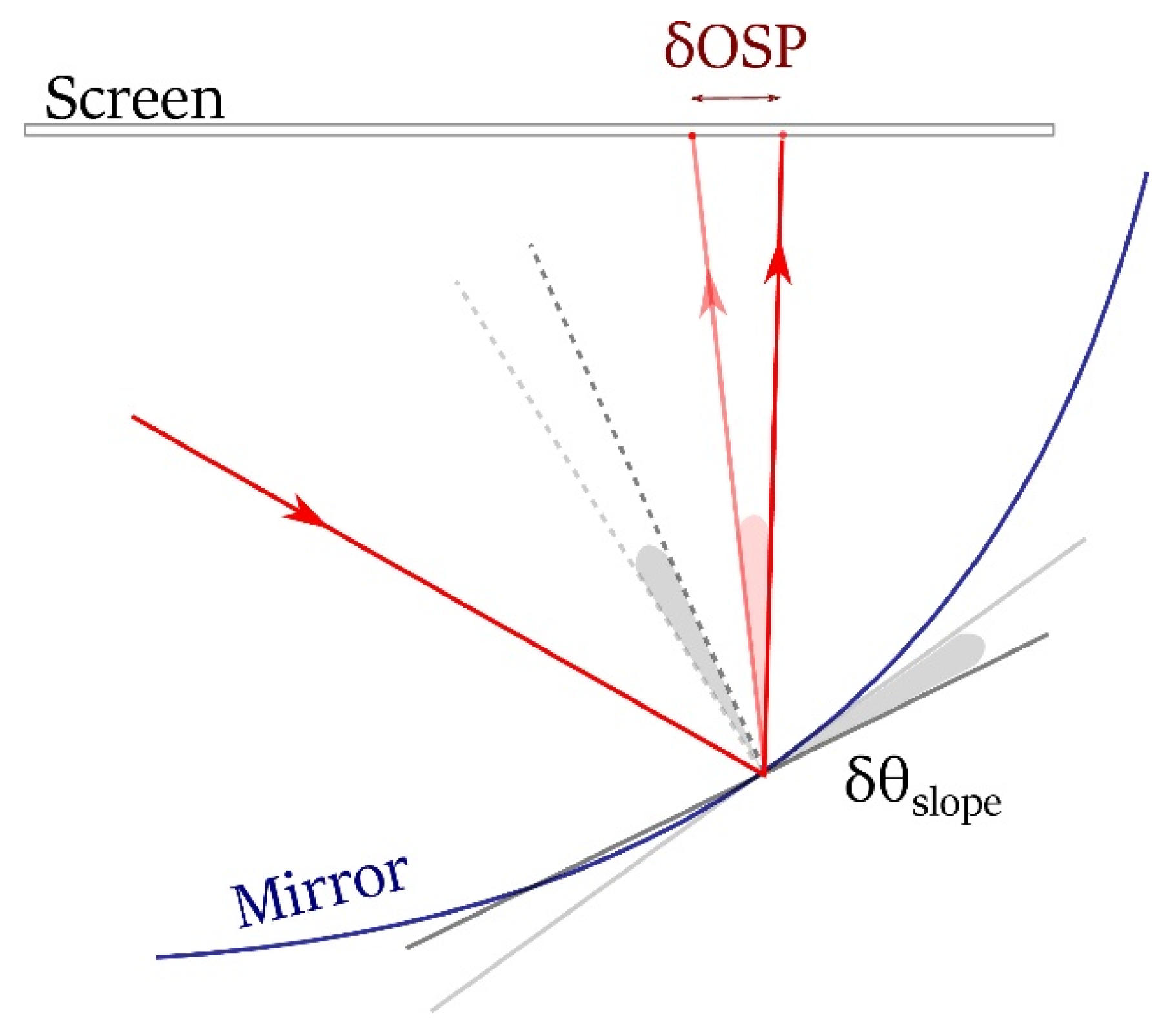
According to the law of reflection, the incident ray and the reflected ray form the same angle with the surface normal and lie in the same plane. For curved surfaces, the direction of reflected rays depends on the local slope of the surface, namely the direction of the line tangent to the curve. A different slope with respect to the ideal one (which can be parametrized by introducing the slope error), could deviate the rays from being intercepted by the receiver. In laser profilometry (LP), a screen (the target) intercepts the ray reflected by the examined mirror surface and the local slope of the surface is calculated after measuring the point where the laser beam intercepts the screen called the on-screen point (OSP) of the laser spot. Referring to Figure 2, for every non-ideal slope, the slope error (δθ_slope) is the angle between this slope and the tangent of the ideal surface. In LP measurements, the slope error (δθ_slope) is derived from the OSP-displacement δOSP of the laser spot with respect to the ideal surface.

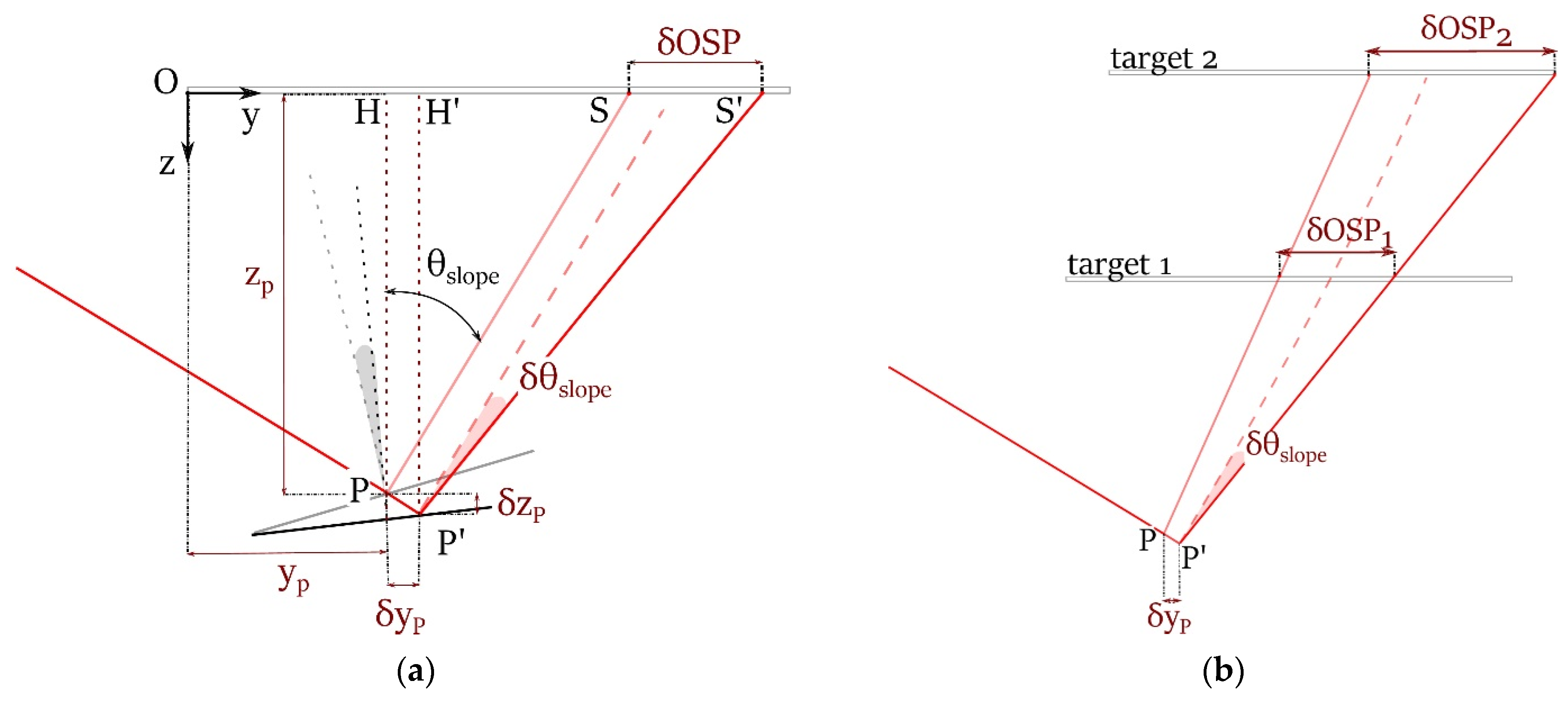
To solve the geometrical problem, the coordinates of the ideal parabola are taken into account. This could be a reasonable approximation if the distance between the examined mirror and the screen is huge with respect to the possible error on the coordinate of the reflection point on the mirror. In other words, it is considered that a variation of the coordinate of the reflection point causes a negligible variation on the OSP of the reflected ray. A simple calculation can be exploited, with reference to Figure 3a, the relationship between coordinate errors, the slope error, and the OSP displacement. The OSP displacements along the x-axis could be neglected because the system is invariant in the longitudinal direction of the receiver tube (along x-axis). Figure 3b compares the slope errors, considering two different distances between the target and the reflecting surface.

In Figure 3a, points P and S represent, respectively, the point of the designed reflector (without any errors) and the relative position of the laser spot on the screen. On the other hand, P’ is the point of the real mirror, resulting from coordinate errors (δz_P, δy_P) and slope errors (δθ_slope), while S’ is the relative on-screen position. In this schema, δOSP is the change in the y coordinates for the laser spot on the screen.

Observing the triangles PHS and P′H′S′:

$$\mathsf{\delta }\mathrm{OSP}=\left({\mathrm{z}}_{\mathrm{P}}+{\mathsf{\delta }\mathrm{z}}_{\mathrm{P}}\right)\cdot \tan \left(\mathsf{\theta }+{\mathsf{\delta }\mathsf{\theta }}_{\mathrm{slope}}\right)+{\mathsf{\delta }\mathrm{y}}_{\mathrm{P}}-{\mathrm{z}}_{\mathrm{P}}\cdot \tan \left(\mathsf{\theta }\right)$$

(1)

where z_P, y_P are the coordinates of the ideal parabola; δz_P, δy_P the coordinate error. From the above formula, the slope error can be written as:

$${\mathsf{\delta }\mathsf{\theta }}_{\mathrm{slope}}=\arctan \left[\frac{\mathsf{\delta }\mathrm{OSP}-{\mathsf{\delta }\mathrm{y}}_{\mathrm{P}}+{\mathrm{z}}_{\mathrm{P}}\cdot \tan \left(\mathsf{\theta }\right)}{{\mathrm{z}}_{\mathrm{P}}+{\mathsf{\delta }\mathrm{z}}_{\mathrm{P}}}\right]-\mathsf{\theta }$$

(2)

If the distance between the target and the reflecting surface increases, δOSP will be greater for a fixed δθ_slope, making δy_P negligible in the formula. Furthermore, z_P would increase as well and δz_P will be negligible (with respect to z_P). Starting from the previous hypothesis (δz_P ≪ z_P and δy_P ≪ δOSP), the slope error could be calculated without considering the coordinate errors:

$${\mathsf{\delta }\mathsf{\theta }}_{\mathrm{slope}}=\arctan \left[\frac{\mathsf{\delta }\mathrm{OSP}+{\mathrm{z}}_{\mathrm{P}}\cdot \tan \left(\mathsf{\theta }\right)}{{\mathrm{z}}_{\mathrm{P}}}\right]-\mathsf{\theta }$$

(3)

Usually, it is possible to give an estimate for the maximum values of δy_P and δz_P and it can be found a suitable distance between mirror and target that makes the coordinate error negligible.

However, neglecting the coordinate error is not always the most precise choice, since it is not legitimate for any position of the target. This could be the case in which the target position is constrained and cannot be placed adequately far from the mirror, as it is in the present case, whose configuration will be described in Section 3 “Experimental Setup”. To get a quantitative idea of the effect, the following argument is proposed.

Firstly, it is assumed that the laser impinges on a point with negligible coordinate errors (δz_P ≈ 0, δy_P ≈ 0) so Equation (1) becomes:

$$\mathsf{\delta }\mathrm{OSP}={\mathrm{z}}_{\mathrm{P}}\cdot \left[\tan \left(\mathsf{\theta }+{\mathsf{\delta }\mathsf{\theta }}_{\mathrm{slope}}\right)-\tan \left(\mathsf{\theta }\right)\right]$$

(4)

Taking into consideration a small slope error (tan(δθ_slope) ≈ δθ_slope) and using the addition formula for the tangent:

$$\mathsf{\delta }\mathrm{OSP}={\mathrm{z}}_{\mathrm{P}}\cdot \left[\frac{\tan \left(\mathsf{\theta }\right)+{\mathsf{\delta }\mathsf{\theta }}_{\mathrm{slope}}}{1+\tan \left(\mathsf{\theta }\right)\cdot {\mathsf{\delta }\mathsf{\theta }}_{\mathrm{slope}}}-\tan \left(\mathsf{\theta }\right)\right]$$

(5)

Considering a reasonable slope error δθ_slope ~ 10⁻³ rad and a target distance of z_P ~ 10⁻¹ m, for tanθ ~ 0 will be δOSP ~ 10⁻⁴ m. In such a case, the OSP displacement will be very small and comparable with the possible coordinate errors, the approximation would not be reliable, and the slope measurement will be inaccurate. As will be seen in the next section, these numbers are typical of our experimental setup, therefore this approximation cannot be used and Equation (3) cannot be applied in the present configuration.

Another possibility was represented by an optical profilometer developed at ENEA by A. Maccari and M. Montecchi [12]. The profile reconstruction can be developed with an iterative method that considers the properties of quadratic functions. In fact, for any two points of a parabola, the abscissa of interception of the tangent lines lies exactly in the middle of the abscissas of the two points. In other words, the approximation says that the behavior between two consequent scanned points has a quadratic form, such as in a Taylor expansion, that is a well reasonable condition. This condition leads to an iterative formula for the reconstruction, where the coordinates are related to those of the closest reconstructed point. For this reason, a first point needs to be measured directly. This approach is the one that has been used for the reconstruction reported in this paper. The calculations developed for this special case are presented in Section 4 “Geometrical Calculation”.

3. Experimental Setup

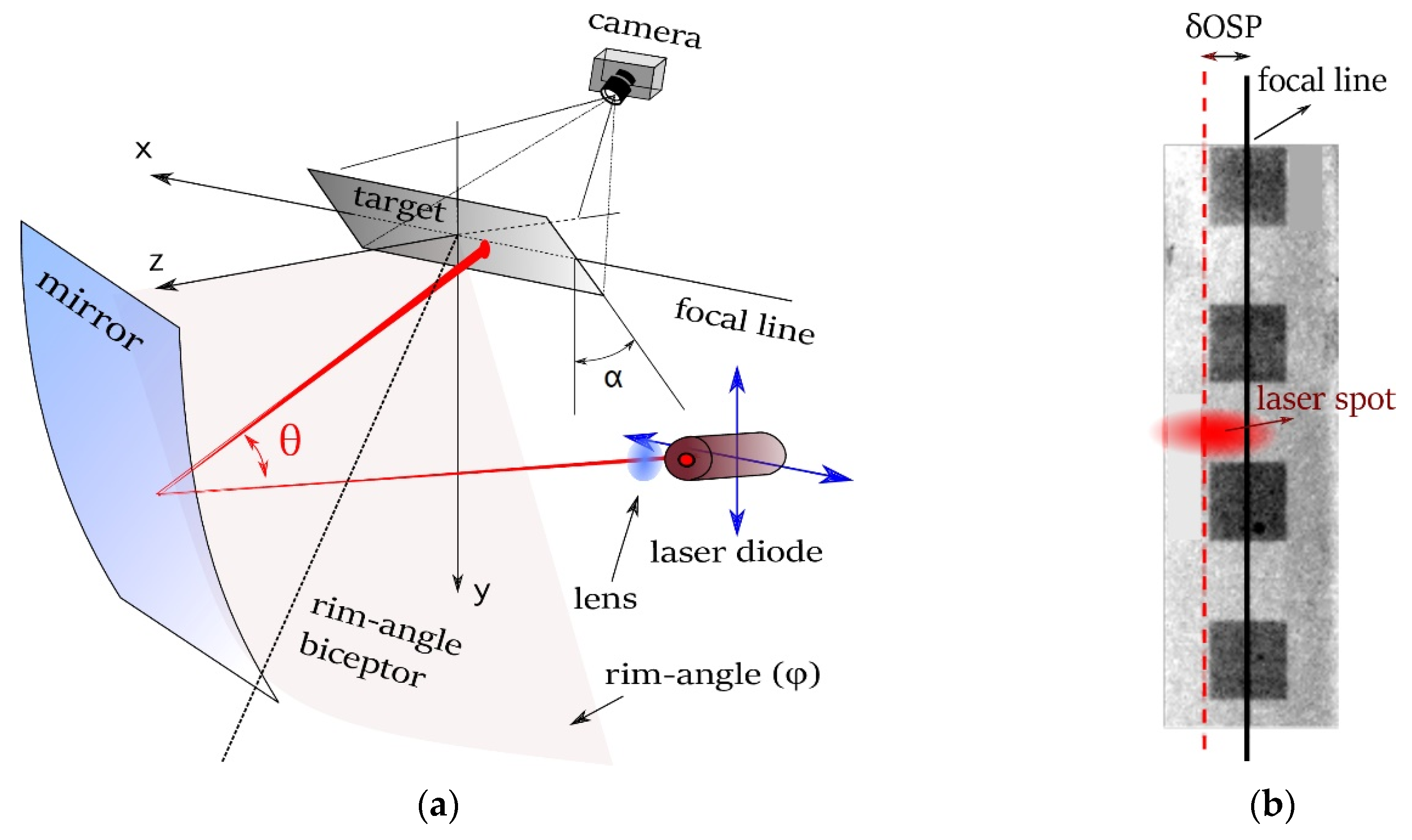
To apply laser profilometry on a micro-parabolic trough collector (m-PTC) the following experimental setup is proposed (Figure 4a). The experimentation has been carried out on the micro-PTC described in Figure 1. The results presented in Section 5, Section 6 and Section 7 refer to measurements performed on the m-PTC of Figure 1 using the experimental setup described in this section.

The collection geometry of this m-PTC has peculiar characteristics that have been especially chosen to have a small and compact collector. The m-PTC profile is a parabola, with the focus under the collector aperture; in fact, the rim angle (φ) exceeds 90°.

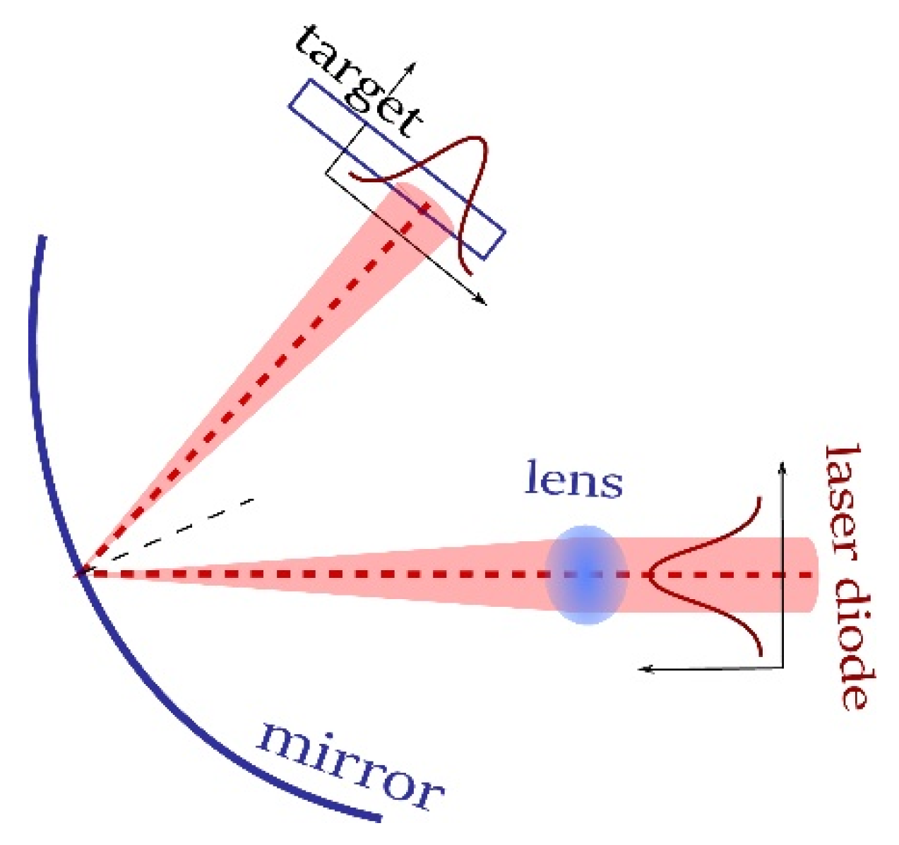
The laser beam is generated by a laser diode that can translate onto a plane parallel to the mirror aperture. The laser diode is a class IIIb laser of LASIRISTM, with a wavelength of 660 nm and an output power of 35 mW. Translation is provided by two automated stages with an accuracy of 2 μm and a range of 150 mm. The laser diode is integrated with a converging lens in front of it. The diameter of the laser spot is about 700 μm in the best focus of the lens, where it has a circular shape.

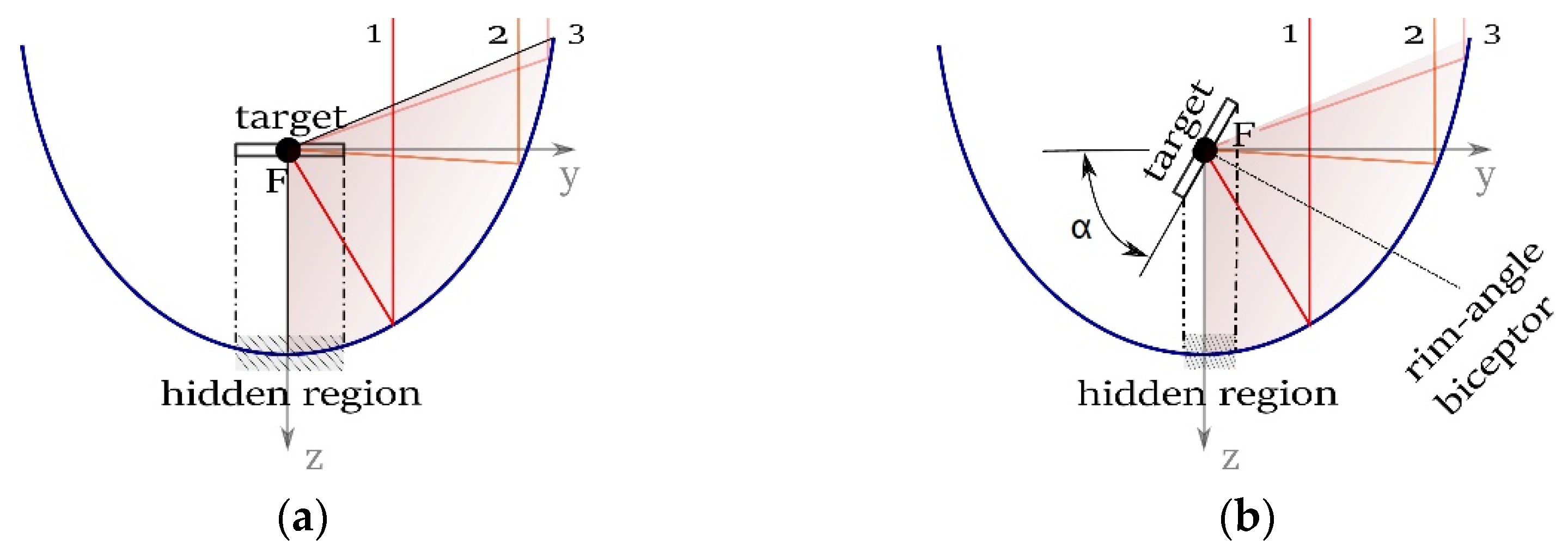
The target in Figure 4a is placed in correspondence to the focal line of the m-PTC and it is tilted at an angle (α) of 51.5° with respect to the mirror aperture plane. This value of α is precisely half of the rim angle and makes the direction of the normal to the target align with the bisector of the rim angle. The rim angle is evidenced in Figure 4a by the light red color. This choice was obliged by the inside position of the focal line, namely the rim angle is greater than 90°. Since the target is inclined, the laser spot becomes an ellipse, as in Figure 4b. In the case of the target parallel to the aperture plane, there would be regions of the mirror surface that reflect light with rays almost parallel to the target surface; an example is shown by ray_2 in Figure 5a. Otherwise, the target tilted at a suitable angle permits that every ray is reflected on the target with an acceptable incidence on it, as shown in Figure 5b. In fact, the rays that are included around ray_2 of Figure 5a fall on an edge of the target even for a correct profile; this complicates the reconstruction algorithm. Instead, by tilting the target, the rays should all fall to the center of the target, as can be seen in Figure 5b, and the reconstruction of the profile is simplified.

The chosen angle is the one that minimizes δOSP for the same slope error. Furthermore, the tilted configuration naturally helps to reduce the hidden region, namely the region of the mirror placed below the target itself. In Figure 5a,b the hidden region is displayed in the grey color, while the rim angle is evidenced by the light red color. In order to convert the pixel measurement of OSP in a physical value (mm), squares of 10 mm per side are printed on the target in Figure 4b. The focal line is printed as well. The OSP is measured using the photo acquisition by a DSLR (camera positioned with the optical axis aligned to the target normal).

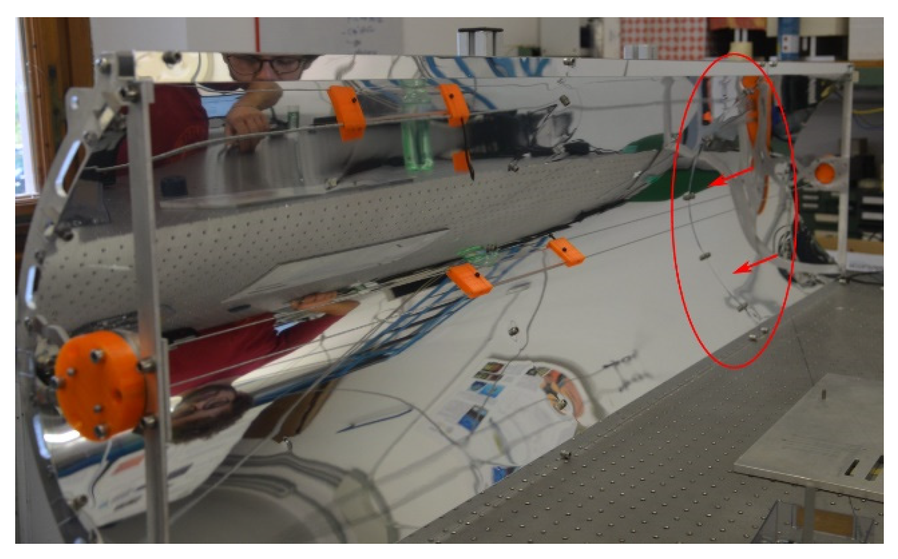
The m-PTC is mounted on an optical table with its aperture placed vertically, so orthogonal to the table, as shown in Figure 6. The accuracy of the positioning of the mirror is verified with a digital inclinometer. Seven measures are performed along the longitudinal direction of the mirror, giving a mean value of (90 ± 0.1°). The target is held on the focal line with two steel cables. The height of the target is constant along the parabolic mirror with a precision of 0.5 mm. For each section of the m-PTC scanned, the inclination of the target is measured by a digital inclinometer with an accuracy of 0.1°. The laser beam needs to be aligned normally to the plane of the mirror aperture. The accuracy of the alignment is 10⁻² mrad.

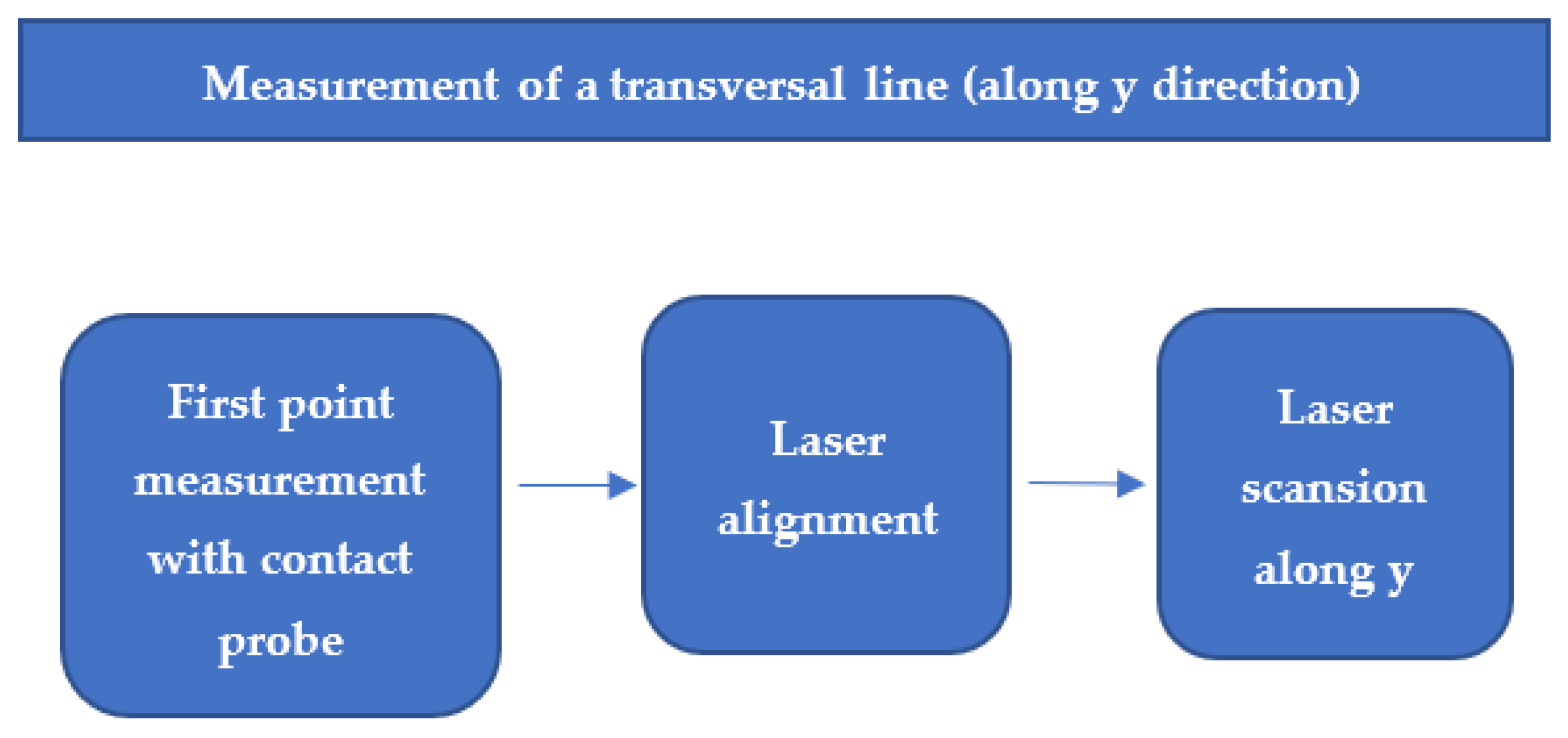
Figure 7 reports a diagram showing the steps of a transversal line measurement. For each section of the mirror, it is necessary to measure a first point to exploit the iterative formula of the reconstruction, as presented in the next section. To do this, a contact probe is utilized with an accuracy of 10⁻³ mm. The probe scans the parabolic mirror for the entire horizontal range, along x direction (see Figure 4a). Data are taken every 5 mm, representing the distance of each transverse section scanned. After the first point is measured, the system can proceed to the laser scanning of the mirror. The laser diode is mounted on two orthogonal micrometric slides (along x and y directions) and for each scanning session, it is moved on the y-axis (see Figure 4a). The scanning is performed in steps of 5 mm.

4. Geometrical Calculation

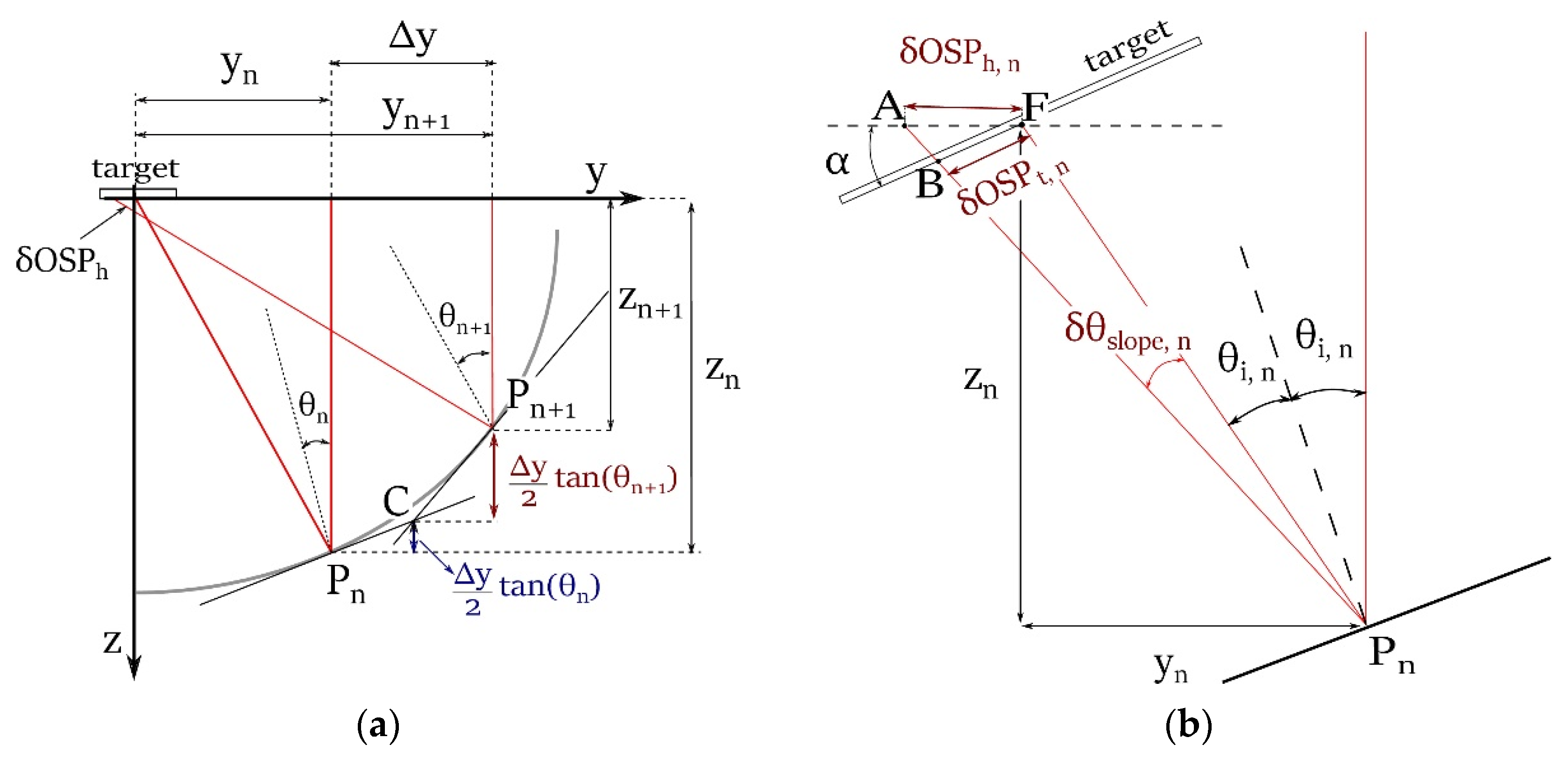
To obtain the formula for the profile reconstruction, it is helpful to start from the classical horizontal configuration shown in Figure 8a. This configuration considers the target placed parallel to the mirror aperture and it is the one mostly cited in the literature. The starting point of these calculations is based on [12,34].

Placing the origin of the coordinates in the focus of the parabola (Figure 8a), for a generic point (P_n) with coordinates y_n, z_n, it is possible to write for the angle of incidence:

$${\mathsf{\theta }}_{\mathrm{n}}=\frac{1}{2}\arctan \left(\frac{{\mathrm{y}}_{\mathrm{n}}+{\mathsf{\delta }\mathrm{OSP}}_{\mathrm{h},\mathrm{n}}}{{\mathrm{z}}_{\mathrm{n}}}\right)$$

(6)

where δOSP_h,n is the OSP displacement for the n-point in the horizontal configuration.

If the coordinates are known, i.e., the coordinate error is negligible, Equation (6) is sufficient to calculate the slope error. Subtracting the value of the incidence angle in the ideal case:

$${\mathsf{\delta }\mathsf{\theta }}_{\mathrm{slope},\mathrm{n}}=\frac{1}{2}\left[\arctan \left(\frac{{\mathrm{y}}_{\mathrm{n}}+{\mathsf{\delta }\mathrm{OSP}}_{\mathrm{h},\mathrm{n}}}{{\mathrm{z}}_{\mathrm{n}}}\right)-\arctan \left(\frac{{\mathrm{y}}_{\mathrm{n}}}{{\mathrm{z}}_{\mathrm{n}}}\right)\right]$$

(7)

Nevertheless, as discussed in Section 2 “Established calculation”, neglecting the coordinate error is not always appropriate. To avoid this issue, the following property of the parabola is considered, as suggested by the work of ENEA [12]. For any two points of a parabola, the abscissa of interception of the tangent lines lies exactly in the middle of the abscissas of the two points. It is possible to write:

$${\mathrm{y}}_{\mathrm{C}}=\frac{{\mathrm{y}}_{\mathrm{n}}+{\mathrm{y}}_{\mathrm{n}+1}}{2}={\mathrm{y}}_{\mathrm{n}}+\frac{\mathsf{\Delta }\mathrm{y}}{2}$$

(8)

and:

$${\mathrm{z}}_{\mathrm{n}+1}={\mathrm{z}}_{\mathrm{n}}-\frac{\mathsf{\Delta }\mathrm{y}}{2}\left[\tan \left({\mathsf{\theta }}_{\mathrm{n}}\right)+\tan \left({\mathsf{\theta }}_{\mathrm{n}+1}\right)\right]$$

(9)

Combining Equation (6) with Equation (9):

$${\mathrm{z}}_{\mathrm{n}+1}={\mathrm{z}}_{\mathrm{n}}+\frac{\mathsf{\Delta }\mathrm{y}}{2}\left\{\tan \left[\frac{1}{2}\arctan \left(\frac{{\mathrm{y}}_{\mathrm{n}}+{\mathsf{\delta }\mathrm{OSP}}_{\mathrm{h},\mathrm{n}}}{{\mathrm{z}}_{\mathrm{n}}}\right)+\tan \left[\frac{1}{2}\arctan \left(\frac{{\mathrm{y}}_{\mathrm{n}+1}+{\mathsf{\delta }\mathrm{OSP}}_{\mathrm{h},\mathrm{n}+1}}{{\mathrm{z}}_{\mathrm{n}+1}}\right)\right]\right]\right\}$$

(10)

This iterative formula is able to give the profile reconstruction starting only form δOSP and the knowledge of the z coordinate of a previous point in the scanning. An initial point has to be directly measured to start the iterative profile reconstruction. To perform this, a contact probe needs to be used.

As exposed before, the present technique is performed on the target tilted of an angle (tilted configuration). To obtain the actual reconstruction formulas, it is sufficient to relate, for each point, the OSP displacement in the horizontal configuration (δOSP) to the one in the tilted configuration (δOSP_t,n). With reference to Figure 8b, observing the triangles ABF and PBF and using the sine law, it is possible to write:

$${\mathsf{\delta }\mathrm{OSP}}_{\mathrm{h},\mathrm{n}}=\frac{{\mathsf{\delta }\mathrm{OSP}}_{\mathrm{t},\mathrm{n}}\cdot \sin \left(\mathrm{A}\hat{\mathrm{B}}\mathrm{F}\right)}{\sin \left(\mathrm{B}\hat{\mathrm{A}}\mathrm{F}\right)}=\frac{{\mathsf{\delta }\mathrm{OSP}}_{\mathrm{t},\mathrm{n}}\cdot \cos \left(\mathsf{\alpha }-{\mathsf{\delta }\mathsf{\theta }}_{\mathrm{slope},\mathrm{n}}-2{\mathsf{\theta }}_{\mathrm{i},\mathrm{n}}\right)}{\cos \left({\mathsf{\delta }\mathsf{\theta }}_{\mathrm{slope},\mathrm{n}}+2{\mathsf{\theta }}_{\mathrm{i},\mathrm{n}}\right)}$$

(11)

Exploiting the addition formula for the cosine, the searched relation is:

$${\mathsf{\delta }\mathrm{OSP}}_{\mathrm{h},\mathrm{n}}={\mathsf{\delta }\mathrm{OSP}}_{\mathrm{t},\mathrm{n}}\cdot \left[\cos \left(\mathsf{\alpha }\right)+\sin \left(\mathsf{\alpha }\right)\cdot \tan \left({\mathsf{\delta }\mathsf{\theta }}_{\mathrm{slope},\mathrm{n}}+2{\mathsf{\theta }}_{\mathrm{i},\mathrm{n}}\right)\right]$$

(12)

Still referring to Figure 8b, examining the triangle PFB, using the sine law and the addition formula for cosines, considering that $\mathrm{F}\hat{\mathrm{B}}\mathrm{P}=\frac{\mathsf{\pi }}{2}+{\mathsf{\delta }\mathsf{\theta }}_{\mathrm{slope},\mathrm{n}}+2{ \mathsf{\theta }}_{\mathrm{i},\mathrm{n}}-\mathsf{\alpha }$ and $\mathrm{PF}=\sqrt{{\mathrm{y}}_{\mathrm{n}}^2+{\mathrm{z}}_{\mathrm{n}}^2}$:

$${\mathsf{\delta }\mathsf{\theta }}_{\mathrm{slope},\mathrm{n}}=\arctan \left[\frac{{\mathsf{\delta }\mathrm{OSP}}_{\mathrm{t},\mathrm{n}}\cdot \sin \left(2{\mathsf{\theta }}_{\mathrm{i},\mathrm{n}}-\mathsf{\alpha }\right)+\sqrt{{\mathrm{y}}_{\mathrm{n}}^2+{\mathrm{z}}_{\mathrm{n}}^2}}{{\mathsf{\delta }\mathrm{OSP}}_{\mathrm{t},\mathrm{n}}\cdot \cos \left(2{\mathsf{\theta }}_{\mathrm{i},\mathrm{n}}-\mathsf{\alpha }\right)}\right]$$

(13)

Equation (13) is an alternative expression for the slope error with respect to Equation (7). In this case it is completely related to measured variables.

Combining Equations (10), (12) and (13), the reconstruction can be performed completely and both the coordinates and the slope error can be calculated. For this aim, a MATLAB^® routine is implemented and the solution of the system of equations is obtained numerically. Uncertainties are estimated with a Monte Carlo method.

5. Measurement of the Spot Position

To measure the spot position on the target, usually a centroid-based method is utilized [12,14]. The centroid of a plane figure is the arithmetic mean position of all the points in the figure. The image is converted into a binary image, namely an image in which the pixel intensity can have a value of 0 or 1. To obtain a binary image, a threshold condition must be imposed. However, this technique can have some drawbacks. First of all, a complete image of the spot has to be provided, otherwise the calculation will lead to a huge error on the spot position. This could occur in the present experimental setup, since the target is a few centimeters wide (to keep small the hidden region as shown in Figure 5) and the spot on the target is about 10 mm wide in one direction. Furthermore, the centroid calculation can be affected by the natural noise on the pixel intensity due to scattering on the spot and/or on the mirror that can affect the shape of the binary image. For this reason, it is impossible to define a suitable uncertainty on the calculation made with this method.

A new technique for the measure of the on-screen point (OSP) of the laser spot is developed. It is based on the variation of the pixel intensity and is not as purely geometric as the centroid method. As shown in Figure 4a, a lens is placed in front of the laser diode. The lens is needed to minimize the laser spot on the mirror; however, on the other side it enlarges the laser spot dimension on the target. This permits to have a well-defined behavior for the pixel intensity on the various pixel positions. The position of the focus center can be calculated as the maximum of the pixel intensity. In fact, the profile of the laser intensity is usually bell-shaped with its maximum located in the center of the beam. Since the laser is focused on the mirror, and the curvature of the parabolic mirror is negligible with respect to the small dimensions of the laser spot, the same profile is found when the spot reaches the target (Figure 9). Furthermore, the maximum of the beam intensity corresponds to the central ray of the laser beam, namely the optic ray that lies on the optical axis of the lens. The central ray has its direction normal to the mirror aperture, so it is suitable for applying the calculations exposed above.

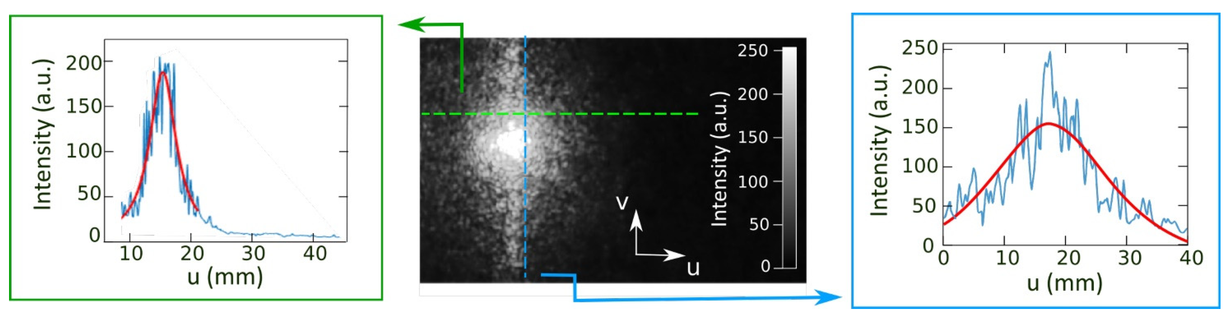
To find the maximum intensity, avoiding that the noise influences the measure, a numerical fit has been performed for both directions of the target u and v (Figure 10). The laser profile is fitted with a Lorentz-like function, here presented for v = constant:

$$\mathrm{f}\left(\mathrm{u}\right)=\frac{{\mathrm{k}}_1}{{\left({\mathrm{k}}_2-\mathrm{u}\right)}^2+{\mathrm{k}}_3}+\mathrm{c}$$

(14)

where k₁, k₂, k₃ are the parameters derived from the fit. The fit is performed for each section of the image, namely for each row (v = constant) and column (u = constant) of the image matrix. The maximum point is then obtained for each fit. The function that represents the behavior of the maximum points is then inferred with a linear function (mean value) and the root mean square is calculated (standard deviation). 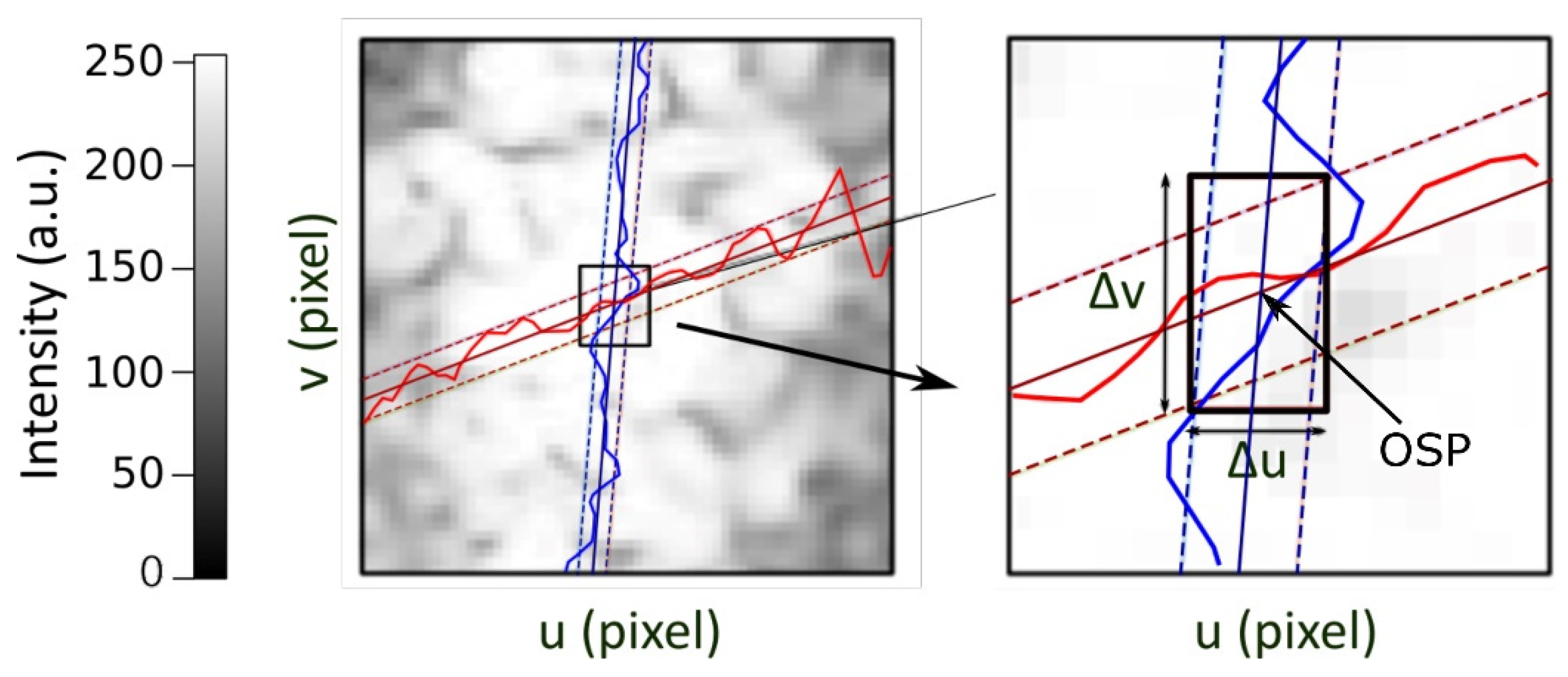Figure 11 shows the enlargement of a measured laser spot as well as the point of maximum for the u-section (red line) and the v-section (blue line), the mean value, and the standard deviations (dashed lines).

The pixel that corresponds to the intersection between the lines represents the expected value for OSP, while the intersection between the standard deviation lines defines the uncertainties Δu, Δv. (Figure 11). Only a section with a well-fitted behavior is considered. To estimate the goodness of fit, the R² statistical parameter, coefficient of determination, is taken into account, only fit with R² > 0.95 are considered. The minimum uncertainty registered is about 200 μm.

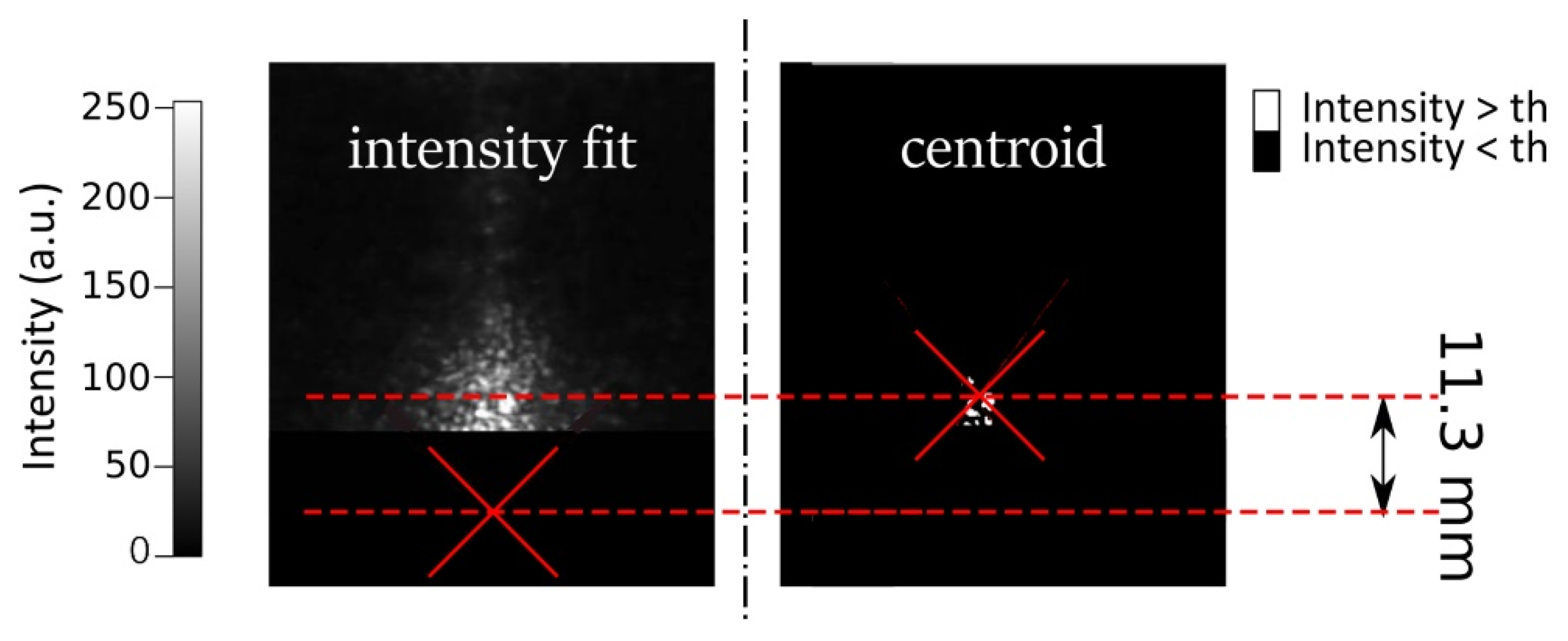
This method, in addition to fully defining the uncertainty for the spot position, has another advantage. To estimate the function that describes the profile of a laser beam it is not necessary to have data for the entire functional behavior. This permits to estimate the center of the spot even when it lies outside the target. This fact makes the target virtually wider. It is worth noting that if the centroid method were used, there would be a huge error in calculating the OSP (Figure 12).

A small portion of the spot in the image produces an increase in uncertainty, but it is a lower error with respect to those obtained by the centroid method. However, due to the iterative nature of the reconstruction formula, it was considered more appropriate to take a more imprecise point than to not take it at all.

6. Reconstruction and Slope-Error Measurement

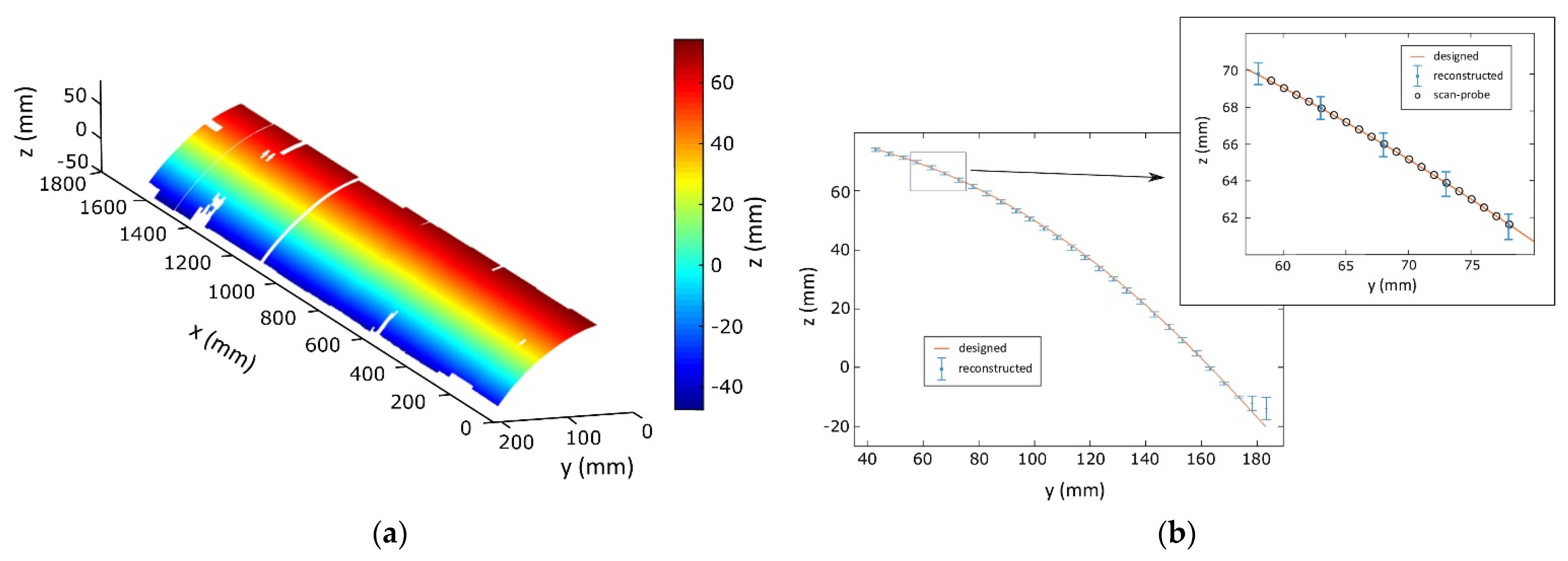
The reconstruction of the mirror is reported in Figure 13a. The points of the reconstruction are not continuous, as happens with the structured light technique [33], but they are at a distance equal to the step of the scanning.

In order to have a validation of the method, several points of the mirror are measured with the contact probe and compared with those obtained with laser profilometry. Figure 13b shows the agreement between the reconstructed points and those measured with the contact probe. The designed parabola is reported as referenced in Figure 13b.

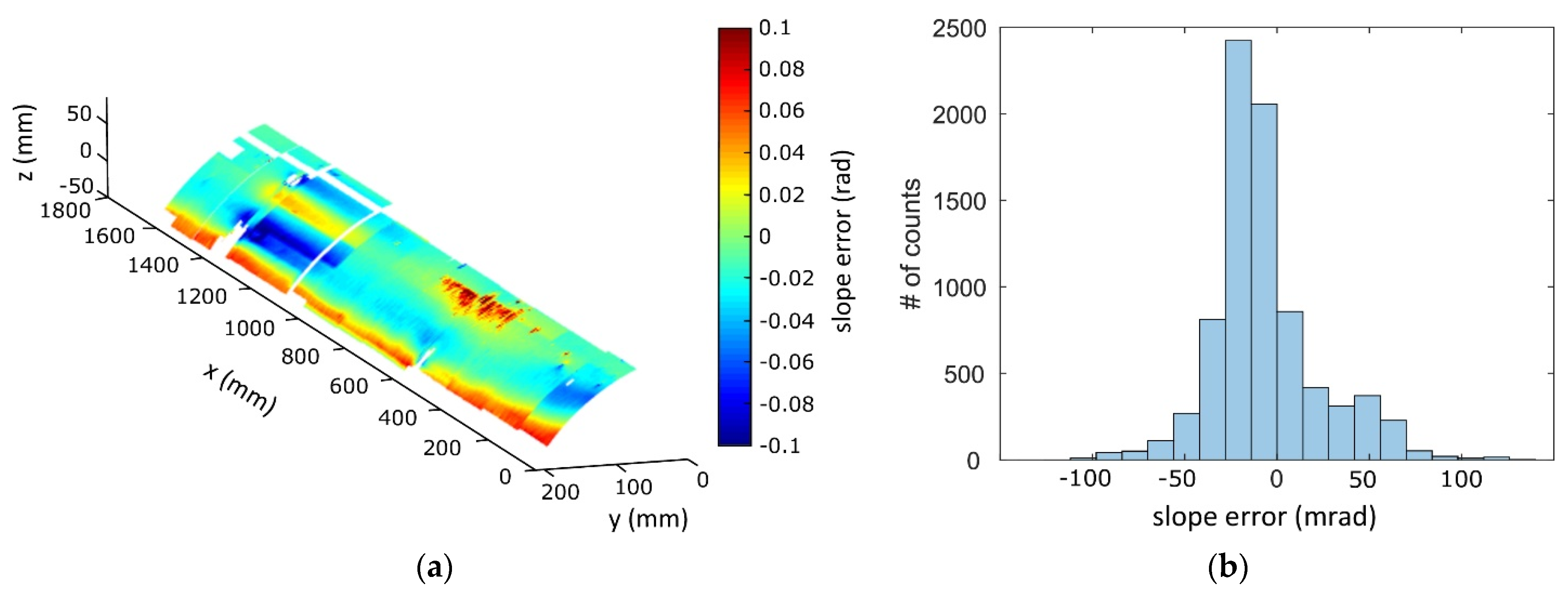
An important parameter in the evaluation of the mirror quality is the slope error (δθ_slope); from Equation (13) it is possible to calculate it for all the reconstructed points. Figure 14a shows the color map of the slope error over the reconstructed points. In the lacking points, it was not possible to carry out the measurement because the measurement requirements were not satisfied. It is a useful diagram to understand the quality of the manufacturing and it clearly shows the region of the mirror with a high value of slope error. In particular, the major defects are mainly located at the rim of the mirror and in a specific region. In every parabolic trough collector, the tensions (due to the deflection of a plane mirror) are discharged at the PTC rim. In practice, the border is always the most defective zone of a PTC.

A peculiar region can be identified for x that lies between 1000 mm and 1400 mm. Three regions with an alternating sign for the slope error (δθ_slope) can be easily noticed in Figure 14a. This corresponds to the conjunction region shown in Figure 6. The center of each region where δθ_slope is negative corresponds to the position of a screw that fixes the reflector to the bearing structure, while a positive slope error is found between them. It is clearly due to the impact of the tension of the reflective material due to the pressure of the screws that are located in that region. This fact underlines the importance of the slope-error measurement in identifying manufacturer defects and their nature.

Analyzing Figure 14a, it can be noticed that the center of each region where δθ_slope is negative corresponds to the position of a screw that fixes the m-PTC reflector to the bearing structure, while the m-PTC upper border is characterized by positive values of δθ_slope.

Figure 14b shows the histogram plot for the distribution of the slope error. The mean value is −6.9 mrad, while its standard deviation is 29.5 mrad.

7. Local Intercept Factor

A parameter fundamental for optimizing the operation of the m-PTC system is the intercept factor, namely the fraction of sunrays reflected by the concentrator that reaches the receiver. It gives an important contribution to the calculation of the optical efficiency of the collector. It permits to assess the quality of the behavior of the light collection. Starting from the results previously shown, it is possible to give an estimate of it.

In fact, knowing the coordinates and the slope error for each reconstruction point makes it possible to evaluate the direction of the reflected ray for that point. Thanks to this, it is possible to evaluate whether, for normal incidences, the ray will be reflected on the surface of the receiver tube.

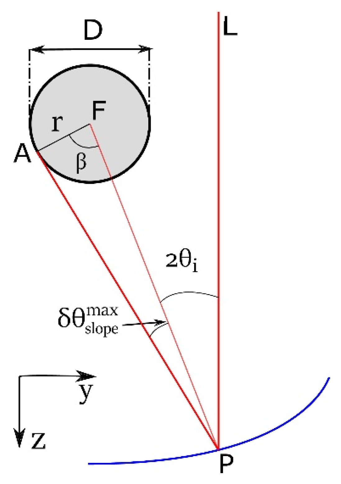
For the ideal position of the absorber tube, the reflected rays will reach its surface at slope-error values lower than a maximum value ${\mathsf{\delta }\mathsf{\theta }}_{\mathrm{slope}}^{\max }$ (Figure 15).

With reference to Figure 15, it is possible to demonstrate that the maximum value ${\mathsf{\delta }\mathsf{\theta }}_{\mathrm{slope}}^{\max }$ occurs for β = 90°. Therefore, observing the triangle PAF:

$${\mathsf{\delta }\mathsf{\theta }}_{\mathrm{slope}}^{\max }=\pm \arcsin \left(\frac{\mathrm{r}}{\mathrm{PF}}\right)=\pm \arcsin \left(\frac{\mathrm{r}}{\sqrt{{\mathrm{y}}_{\mathrm{n}}^2+{\mathrm{z}}_{\mathrm{n}}^2}}\right)$$

(15)

where r is the radius of the absorber tube and the value is considered both for positive and negative angles. Comparing the calculated slope error it is possible to estimate whether the reflected ray impinges on the absorber tube or not. In particular, the condition is:

$$\left|{\mathsf{\delta }\mathsf{\theta }}_{\mathrm{slope}}\right|<\left|{\mathsf{\delta }\mathsf{\theta }}_{\mathrm{slope}}^{\max }\right|$$

(16)

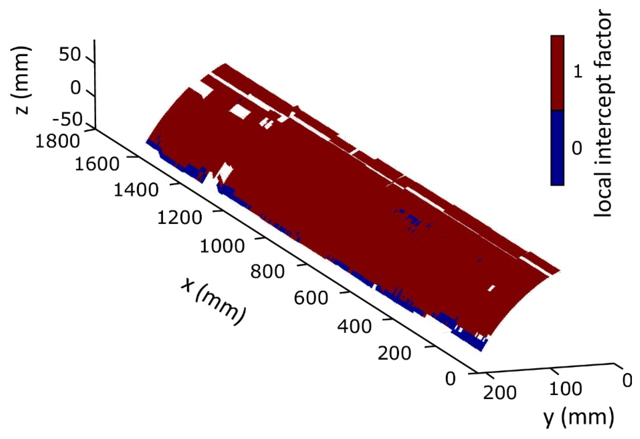
Starting from this condition, it is possible to assign for each point of the reconstruction a binary variable that is 1 if the condition is true and 0 otherwise. Here, this variable is called the local intercept factor (ϓ_local). A map of the local intercept factor over the reconstructed surface is shown in Figure 16.

As Figure 16 shows, the local intercept factor is a good parameter to estimate the local quality of the mirror. It is able to detect zones of the mirror where the defects are such that the mirror surface is useless, namely these zones do not reflect the radiation into the receiver tube. In our case, the mapping of the local intercept factor shows the presence of systematic defects near the rim of the mirror. This manufacturing defect causes optical losses in the system and consequently a decrease in the intercept factor. On the other hand, not all the defects identifiable from the slope error map (Figure 14a) give a zero contribution to the intercept factor. As can be easily seen, the conjunction region at 1000 mm < x < 1400 mm does not negatively affect the intercept factor. Furthermore, the region at the rim of the collector with a zero local intercept factor is smaller than that which could be estimated by looking at the slope error map.

In other words, this calculation shows that there is an acceptance threshold for the combination of slope and coordinate errors. For example, the tension on the surface given by the screws on the mirror does not influence the optical efficiency of the collector.

The mean value of the local intercept factors, measured with this technique, is 0.91 and it is called the global intercept factor. It is worth noting that this value only considers the profile contribution to this factor and the receiver tube is assumed to be in the ideal position. This value is in agreement with the results obtained with a measurement performed using a different technique on the same object [33]. If the solar half angle of 0.27° at the earth’s surface is taken into account in the calculation of the intercept factor, the value is 0.89. This reduction from 0.91 is due to the fact that the angle ${\mathsf{\delta }\mathsf{\theta }}_{\mathrm{slope}}^{\max }$ becomes smaller, thus less rays impinge on the tube.

8. Conclusions

A micro-PTC has been designed with a mirror size smaller than usual, because it is conceived to minimize costs, with an approach similar to that which occurs for photovoltaic systems: size reduction and standardization. Micro-PTC prototypes have been fabricated; however, the constructed object can never be identical to the designed object.

The peculiar size and shape of this micro-PTC was made necessary to develop a tailored technique of laser profilometry. The proposed control method is devoted to being used during the manufacturing phase of the parabolic collector.

A laser beam impinges on the mirror surface and its reflection is recorded on a target placed on the focal line of the m-PTC. The position of the reflected spot (on screen point (OSP)) with respect to the focal line gives information about the slope of the parabolic mirror examined.

The target is located on the focal line in order to minimize the hidden region, even if this choice allows to examine half of the parabolic mirror at a time.

A suitable approximation has permitted the implementation of an iterative formula for the profile reconstruction, which has been numerically calculated. This formula requests the knowledge of the coordinates of a first point provided by a very accurate contact probe.

Thus, the final implementation of this method used for the m-PTC includes a laser diode, able to translate over the parabolic mirror aperture, with a converging lens placed in front of it. The presence of the lens ensures that the beam reflection is not affected by the mirror curvature, but the spot reflected on the screen does not have a circular shape. After a deep analysis of the various spots, it was possible to make an improvement in the calculation of the spot position. This new method also permits to infer the center of the spot even if it is outside the target, giving it a virtual expansion.

The result of the calculation is the reconstruction of the 3D profile of half of the m-PTC and a map of the slope error (δθ_slope) for each point of the m-PTC surface. This last graph is very important in evaluating the profile realization of the m-PTC samples.

Further calculations permit to estimate, for each point, the contribution to the intercept factor, called the local intercept factor. It can be noticed that the portions of surface that do not contribute to focus the solar rays on the tube are quite small and distributed mainly at the edges of the parabolic mirror.

The global intercept factor is calculated averaging the values of the local intercept factor, giving a value of 0.91. This value is consistent with a measurement on the same object obtained with a different technique [33].

The proposed methodology is able to provide useful information about the location of the parts of the mirror that could bring optical losses. From the study of the local intercept factor, a zone of systematic defects on the rim of the parabolic mirror must be evidenced. This information could be useful for the improvement of the bearing structure of the reflectors.

A possible evolution of this technique would avoid the use of the contact probe by substituting the coordinates of the position of the first point with the direct measurement of the slope angle; it would be measured directly on the laser beam by using optical angular gauges.