Abstract
In recent years, scale-by-scale energy transport in wall turbulence has been intensively studied, and the complex spatial and interscale transfer of turbulent energy has been investigated. As the enhancement of heat transfer is one of the most important aspects of turbulence from an engineering perspective, it is also important to study how turbulent heat fluxes are transported in space and in scale by nonlinear multi-scale interactions in wall turbulence as well as turbulent energy. In the present study, the spectral transport budgets of turbulent heat fluxes are investigated based on direct numerical simulation data of a turbulent plane Couette flow with a passive scalar heat transfer. The transport budgets of spanwise spectra of temperature fluctuation and velocity-temperature correlations are investigated in detail in comparison to those of the corresponding Reynolds stress spectra. The similarity and difference between those scale-by-scale transports are discussed, with a particular focus on the roles of interscale transport and spatial turbulent diffusion. As a result, it is found that the spectral transport of the temperature-related statistics is quite similar to those of the Reynolds stresses, and in particular, the inverse interscale transfer is commonly observed throughout the channel in both transport of the Reynolds shear stress and wall-normal turbulent heat flux.
1. Introduction
Analysing the budgets of the Reynolds stress transport equation is a useful tool for investigating turbulence transport phenomena as it shows quantitatively where and how much turbulence is produced from the mean flow, redistributed among different velocity components by the effect of pressure, dissipated into heat by viscosity, etc. A particularly interesting feature is that the budget includes spatial transport (or diffusion) terms, which do not lead to total energy gain/loss of turbulent energy across the flow field but represent spatial transports by different effects, namely, advection by the mean flow and diffusion by turbulence, pressure fluctuation and viscosity. Similarly to the Reynolds stress transport equation, one can derive the transport equations of passive-scalar fluxes, and one of the most engineering-relevant features of turbulence to enhance the spatial transport of heat and mass may be expressed by the turbulent diffusion terms in these transport equations.
The budget analysis of the Reynolds stress (or turbulent kinetic energy) transport equation has recently been extended to scale-by-scale budget analysis, where the transport equation is decomposed into large- and small-scale parts (e.g., Refs. [1,2,3,4,5]) or the spectral transport equation [6,7,8] is derived. Similar analysis of the energy transport at each scale is also possible based on the transport equations of two-point correlation quantities, such as the second-order structure function (e.g., Refs. [9,10,11]). The main feature of such scale-by-scale budget analysis is that the turbulent diffusion term is split into the spatial diffusion at each scale and the interscale transport at each spatial location, which allows us to separately investigate the spatial and interscale transfer effects by the nonlinear scale interaction of turbulence.
Such scale-by-scale budget analysis of the turbulent energy transport has been used to study the complex energy transport in wall turbulence, and the behaviour of the interscale energy transport term was focused on in relation to the dynamics of coherent structures in the inner and outer layers. Particularly, in the spectral analysis of the energy transport, the analysis is possible based on either the streamwise and spanwise Fourier modes, and the interscale energy transport observed through the Fourier modes in different directions may represent different physical phenomena. It was suggested in Ref. [4] that the interscale energy transfers in the streamwise length scales likely represent the energy transfer associated with the self-sustaining cycles of each coherent structure in the inner and outer layer. On the other hand, the interscale energy transfers observed through the spanwise Fourier modes may represent the interactions between the inner and outer coherent structures. Many of the earlier studies on the scale-by-scale budget analysis were based on spanwise length scales, as the inner and outer structures have clearly different spanwise length scales [12]. It has been shown that the interscale energy transport terms exhibit both forward (from larger to smaller scales) and backward (from smaller to larger scales) energy transfers in the near-wall region [1,3,6,11,13,14], unlike in homogeneous isotropic turbulence, where the energy transfer is basically from larger to smaller scales. In particular, among these earlier studies, Kawata and Alfredsson [1] experimentally investigated a turbulent plane Couette flow and showed that the Reynolds shear stress is transferred from relatively small scales near the wall to large scales away from the wall. This observed transport of the Reynolds shear stress can be interpreted as the bottom-up influence from the inner to outer structure, which is in contrast to the general picture of turbulence that the energy is basically transferred from larger to smaller scales. Although the physical phenomenon represented by the inverse interscale transfer of the Reynolds shear stress has not been fully elucidated yet, some recent studies have suggested that the interscale energy transfer in the spanwise length scales is related to the interaction between the inner and outer structures [3,11,15].
The scale-by-scale analysis of the passive-scalar fluxes can also be performed in the almost same manner as the analysis of the Reynolds stress transport as their transport equations are similar. Such scale-by-scale analysis of passive-scalar transfer allows us to investigate the interscale and spatial transport of the passive scalar caused by nonlinear interactions between different scales in the velocity fields. However, despite numerous studies reported on the wall turbulence with a passive scalar field (e.g., Refs. [15,16,17,18,19,20,21,22,23,24]) in the last few decades, the scale-by-scale transport of the passive scalar in wall turbulence has not been explored yet.
In the present study, we extend the spanwise spectral analysis on the Reynolds stress transport in Ref. [1] to the turbulent heat flux transport. The transport equation budgets of the temperature-related spectra are investigated based on the direct numerical simulation (DNS) data of wall turbulence with a passive-scalar heat transfer, particularly focusing on if the transport from smaller scales near the wall to larger scales away from the wall is also investigated for turbulent heat fluxes similarly to the Reynolds stress transport. Turbulent plane Couette flow is chosen as the test case, because very-large-scale structures filling up the entire channel appear at relatively low Reynolds numbers [25,26,27,28,29,30,31], and therefore, scale separation between the inner and outer structures is relatively clearer than in other canonical wall-bounded flow configurations at the same Reynolds number. The constant-temperature-difference condition is adopted as the thermal boundary condition on the walls so that the mean velocity and temperature profiles are similar to each other. Then, fluctuating velocity and temperature fields are compared by focusing on the similarity/difference in the interscale and spatial energy transport caused by scale interactions. The analysis is based on the DNS data provided in our previous work [32], where the streamwise Fourier mode analysis was performed, and thereby, the interscale energy transfers associated with the self-sustaining cycle of coherent structures were compared for the velocity and temperature fields. In this study, on the other hand, the spanwise spectral analysis is performed on the transport of the turbulent heat flux, and the interscale transfer of turbulent heat fluxes in spanwise length scales is investigated in relation to the interactions between the coherent structures in the inner and outer layers.
The layout of this paper is as follows: In Section 2, the numerical setup for the DNS is briefly described, and the spectral transport equations of the temperature-related statistics are introduced. In Section 3, the results of the spectral budget analysis are presented. First, the distributions of the turbulent energy and temperature-related spectra are shown, followed by the corresponding interscale and spatial fluxes. Then, the budget balance of the transport equations of the temperature-related spectra are investigated in comparison with those of the corresponding Reynolds stress component. Finally, in Section 4, a discussion and concluding remarks are given.
2. DNS Dataset and Spectral Budget Analysis
2.1. DNS Dataset of a Turbulent Plane Couette Flow with Temperature Transport
In the present study, the budget analysis of the spectral transport equations is performed with a DNS dataset of a turbulent plane Couette flow with passive-scalar temperature transport obtained in our previous work [32]. Here, we briefly summarise the computational conditions. The geometrical configuration of the plane Couette flow is such that a shear flow is driven by the stationary bottom wall and the top wall translating with a constant speed , which are separated by a distance h. The x-, y-, and z-axes are taken in the streamwise, wall-normal, and spanwise directions, and the origin of the coordinates is placed on the stationary bottom wall; the bottom and top walls are located at and , respectively. The temperatures of the walls are uniform and constant in time, and the temperature difference is ( and are the temperature of the top and the bottom walls, respectively).
The governing equations of fluid flow are the continuity and Navier-Stokes equations for incompressible flow that are non-dimensionalised by h and , and the convection-diffusion equation of passive-scalar temperature non-dimensionalised by , h, and is solved for the fluctuating temperature field. A non-slip boundary condition is applied to the fluid velocity on the wall, and as described above, the temperature on the walls is uniform and constant in time with the temperature difference . It should be noted here that both the velocity and temperature fields are driven by a uniform and constant velocity or temperature difference between the top and bottom walls, and therefore, the boundary conditions on the walls for the velocity and temperature fields are similar when scaled by the velocity difference and the temperature difference , respectively. For the streamwise and spanwise directions, periodic boundary conditions are applied. The Reynolds number and Prandtl number are and , where and are the kinematic viscosity and the thermal diffusivity of the fluid, respectively, and other details of the DNS, such as the domain size and spatial resolution, are listed in Table 1.

Table 1.
Computational conditions: streamwise and spanwise domain lengths, number of grid points, spatial resolutions, and the friction Reynolds number (, ). The Reynolds number and Prandtl number are and , respectively.
We denote the velocity components in the x-, y-, and z-directions as , v, w, respectively. Here, U is the mean streamwise velocity, and the lower-case letter represents the fluctuation around the mean value of each velocity component (note here that the mean wall-normal and spanwise velocities are zero). The temperature is defined as the temperature difference between the fluid and the bottom wall and denoted as : here, and are the mean temperature and the temperature fluctuation, respectively, and and at the bottom and top walls, respectively. In the following, ⟨⟩ represents averaged quantities obtained by averaging in x- and z-directions and in time. They are also averaged between the lower and upper half of the channel because of the symmetric flow configuration.
Figure 1 and Figure 2 show the profiles of the mean velocity and temperature and those of the second-order statistics, such as velocity and temperature variances and their cross correlations. Here, used in Figure 1b is the friction temperature defined as , where and are the mean heat flux on the wall and the specific heat at constant pressure, respectively, and is the friction velocity defined as ( and are the wall shear stress and the fluid density). As shown in Figure 1a, the profile of the mean temperature is anti-symmetric, similarly to the mean velocity profile due to the similar boundary conditions for the velocity and temperature fields, and it is also seen in Figure 1b that the mean temperature gradient in the vicinity of the wall is markedly smaller than the mean streamwise velocity gradient . This difference can be attributed to the fact that , which makes the effect of molecular diffusion more significant in the temperature field than in the velocity field.
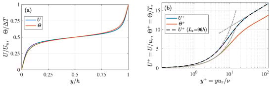
Figure 1.
Profiles of mean streamwise velocity U and the mean temperature in (a) outer and (b) inner scaling. In panel (b), the grey chained lines indicate and for the mean velocity profile and for the mean temperature profile, and the black dashed line presents the profile of mean velocity obtained with an extremely large computational domain (96.0 h, 12.8 h) in Ref. [4].
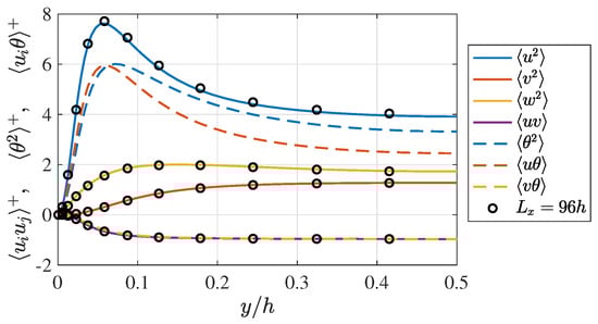
Figure 2.
Profiles of (solid lines) the Reynolds stresses and (dashed lines) the temperature-related turbulent statistics and . The values are scaled based on the inner units, and/or , and only is shown. The black circles present profiles of the Reynolds stresses obtained with an extremely large computational domain (96 h, 12.8 h) in Ref. [4].
Figure 2 presents the profiles of the Reynolds stresses , , , and , and the temperature-related statistics: the temperature fluctuation and the velocity-temperature correlations and . As shown here, the temperature fluctuation and the streamwise-velocity-temperature correlation have similar profiles to the streamwise velocity fluctuation , which indicates a certain similarity between the fluctuations of the streamwise velocity u and of the temperature . This is attributable to the fact that the profiles of the mean streamwise velocity U and mean temperature are similar. It is also shown here that the profiles of the Reynolds shear stress and turbulent heat flux are almost on top of each other, which indicates a strong similarity between the turbulent momentum and the heat transfers. It should be noted that the cross correlations related to the spanwise velocity w, such as and , are negligibly small in magnitude compared to and , although the spanwise velocity variance is certainly larger than that of the wall-normal velocity , and these cross correlations related to w are, therefore, not investigated in the present study.
In the DNS of turbulent plane Couette flow, one needs to use a considerably large computational domain to exclude the dependency of the obtained DNS results on the computational domain size due to the very-large-scale structure [25]. The effect of the domain size was carefully addressed in our previous work [4], and it was confirmed that the domain size used for obtaining the present DNS dataset, h, 12.8 h), was large enough to exclude the domain-size effect, as demonstrated in Figure 1 and Figure 2 by the good agreement between the present computational results and those obtained with a much larger computational domain in Ref. [4].
2.2. Spectral Analysis of the Reynolds-Stress Transport and Turbulent Heat Transfers
In the present study, the spectral transports of the temperature fluctuation and the turbulent heat fluxes are analysed based on spanwise Fourier mode analysis. The transport equations of the temperature-related spectra are derived similarly to those for the Reynolds stress spectra. Here, the derivation of the transport equations of the Reynolds stress spectra is briefly reviewed, and the spectral transport equations for the temperature-related statistics are introduced by similar means.
2.2.1. Transport of Reynolds Stresses
The transport of the Reynolds stresses is expressed as
where the terms on the right-hand side are the production (), viscous dissipation (), pressure-gradient work (), viscous diffusion (), and turbulent diffusion () terms, which are defined as
The pressure term may be decomposed into the pressure-strain correlation and the pressure diffusion :
is the Kronecker’s delta.
Now, we introduce a decomposition of the fluctuating components into their large- and small-scale parts as
based on the spanwise Fourier-mode decomposition, where and consist of the spanwise Fourier modes at smaller wavenumbers than a cutoff wavenumber , while and comprise the rest: , . With such a decomposition, there is no overlapping wavenumber range between the large- and small-scale quantities. Hence, the cross correlation between them is zero for any combination of quantities:
Equation (6) is mathematically satisfied if the decomposition (5) is based on an orthogonal mode decomposition and the large- and small-scale quantities do not have any mode in common, which is the case in the present study. Similar decomposition is also possible based on other orthogonal mode decomposition methods, for example, the proper orthogonal mode decomposition.
As the cross correlations between the large- and small-scale quantities are zero as described above, the Reynolds stresses are decomposed simply into their large- and small-scale parts as
and by a similar manner, to derive the “full” Reynolds stress Equation (1), one obtains the transport equations of the large- and small-scale parts of the Reynolds stresses (the details of the derivation are found in Refs. [4,33]) as
The terms on the right-hand sides of Equations (8) and (9) are the large- and small-scale parts of their counterpart in Equation (1), except for . In particular, the first four terms on the right-hand side of each equation (i.e., the production, viscous dissipation, pressure-gradient work, and viscous diffusion) are simply decomposed into their large- and small-scale parts, similarly to the Reynolds stress decomposition in Equation (7): these terms in Equation (8) are defined as those in Equations (1)–(3) with and replaced by and (the corresponding terms in Equation (9) are similarly defined by and ).
On the other hand, the turbulent diffusion is decomposed as
where and are, respectively, the large- and small-scale part of the triple velocity correlation defined as
Note here that the triple correlations in Equations (11) and (12), including both the large- and small-scale parts, such as and , are not zero unlike the second-order cross correlations and . The last term in Equations (8) and (9), , is defined as
It is observed from Equations (8) and (9) that this term appears in the transport equations of both and with different signs, which means that represents the energy flux between the large- and small-scale velocity fields across the cutoff wavenumber .
It is worth pointing out here that only the turbulent diffusion terms ( and ) and the interscale energy flux term () include both the large- and small-scale parts of the fluctuating velocities, whereas the other terms in the transport equations consist of either the large- or small-scale part only. This is because the turbulent transport and the interscale energy flux terms are the third-order moments of the fluctuating velocities (and the velocity gradients), while the other terms are second-order moments. These terms including both the large- and small-scale parts of the fluctuating velocity can be interpreted as the energy transport effects by interactions between different scales: the turbulent transport ( and ) indicates the energy transport in physical space caused by scale interactions, while the interscale energy flux () is the energy transport between different scales.
As the large-scale part of the Reynolds stresses and the spanwise one-dimensional spectra of the Reynolds stresses are related as
the transport equations of the Reynolds-stress spectra can be derived by differentiating both sides of Equation (8) with respect to as
where the terms on the right-hand side are the -derivatives of the counter parts in Equation (8). The first five terms represent the spectra of the corresponding terms of Equation (1): the spectra of the production (), viscous dissipation (), pressure term (), viscous diffusion () and turbulent diffusion () terms. The interscale transport term represents the energy gain/loss by the interscale flux at each wavenumebr . According to Equation (4), the pressure-gradient-work spectrum can also be decomposed into the spectra of the pressure-strain energy redistribution term and the pressure diffusion term as
The turbulent spatial transport and the interscale transport , which are of particular interest in the present study, are defined as
Here, is the spectra of triple velocity correlations defined as
As the physical meaning of is the spatial transport flux of the Reynolds stress in the -direction caused by the velocity fluctuation , their spectra represent the spatial flux of the Reynolds stresses in the -direction at each spanwise wavenumber.
In order to evaluate the terms on the right-hand side of Equation (10), the procedure to decompose the velocity and temperature fluctuations as in Equations (5) by applying a spatial filter is repeated for all possible values of , i.e., , and all terms on the right-hand side of Equation (8) are evaluated for each value of the cutoff wavenumber . Then, the derivatives with respect to are evaluated for all terms at each , and thus the terms on the right-hand side of Equation (10) are obtained as functions of the wall-normal position y and the spanwise wavenumber (or the spanwise wavelength ).
2.2.2. Transport of Temperature Fluctuation and Velocity-Temperature Correlations
Now, we derive the spectral transport equations of the temperature-related turbulence statistics. The transport equation of the temperature fluctuation is written similarly to the Reynolds stress Equation (1) as
with the production (), viscous dissipation (), viscous diffusion (), and turbulent transport () terms defined as
The transport equation of the turbulent heat fluxes is also similarly obtained as
with the production (), viscous dissipation (), pressure-gradient-temperature correlations (), viscous diffusion (), and turbulent diffusion () terms defined as
Based on the decomposition given by Equation (5), the temperature variance and the turbulent heat fluxes are also split into their large- and small-scale parts, similarly to the Reynolds stress decomposition (7), as
Therefore, the transport equations of their large- and small-scale parts can be derived similarly to Equations (8) and (9). Then, these large- and small-scale parts of the temperature-related statistics are related to their spectra, similarly to Equation (14), as
and the transport equations of these temperature-related spectra can also be obtained by differentiating the equations of and . With such procedures, one obtains the temperature-variance spectrum equation as
with the terms on the right-hand side representing the spectra of the counterparts in Equation (19). The interscale and the turbulent spatial transport terms are defined as
where and are the interscale and spectral spatial fluxes of the temperature fluctuation defined as
with and being the large- and small-scale part of the spatial flux of the temperature fluctuation :
Similarly, the transport equation of the turbulent heat flux spectrum is obtained as
and the terms on the right-hand side are, again, the spectra of their counterparts in Equation (21). The interscale and the turbulent spatial transport terms are defined in the same manner as in other spectral transport equations:
where the interscale flux and spectral spatial flux are, respectively, defined as
Here, and are the large- and small-scale parts of defined as
The terms on the right-hand side of Equations (17) and (19) are obtained in a similar manner as those of Equation (10): Repeating the decomposition (5) for all possible values of the cutoff wavenumber , evaluating all terms in the transport equations of and at each , and evaluating the -derivatives of all terms at each .
3. Results
3.1. Spectra of Temperature-Related Statistics and Their Interscale and Spatial Transports
Figure 3 presents the distributions of the spanwise one-dimensional spectra of the streamwise turbulent energy , temperature fluctuation , and temperature-velocity correlation in the premultiplied form. The distribution of the streamwise turbulent energy spectrum in the panel (a) shows two significant energy concentrations, one of which is the energy peak located in a relatively small wavelength range near the wall around and the other is the broad energy band at a large wavelength around covering most of the channel. Here, is the spanwise wavenumber scaled by viscous length scale . These energy peaks clearly correspond to the small-scale coherent structures near the wall and the very-large-scale structure of plane Couette turbulence, respectively. As shown in this figure, the energy peaks corresponding to these coherent structures at different scales are observed to be clearly separated from each other despite the relatively small Reynolds number , which is a unique feature of plane Couette turbulence [26,27,28].
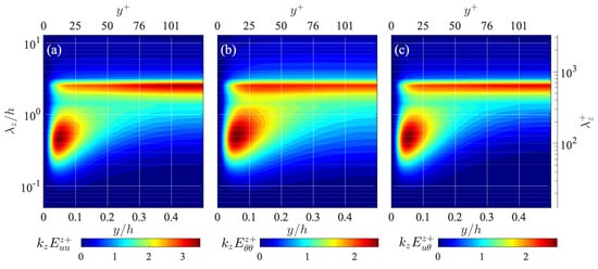
Figure 3.
Space-wavelength () diagrams of spanwise one-dimensional premultiplied spectra of (a) streamwise turbulent energy , (b) temperature fluctuation , and (c) velocity-temperature correlation . The values are scaled by , , and , respectively.
The temperature-fluctuation spectrum presents a similar distribution to the streamwise turbulent energy , as shown in Figure 3b, in which the energy peaks corresponding to the near-wall and very-large-scale structures are indicated at almost the same position in the y- diagram. The location of the near-wall peak is, however, at a slightly larger wavelength and further from the wall than the corresponding peak in the distribution, , which can be attributed to the more significant effect of molecular diffusion in the temperature field as . The distribution of the temperature-velocity cospectrum also shows a similar distribution to , indicating similar behaviours of the fluctuating streamwise velocity and temperature.
Figure 4 compares the spanwise one-dimensional cospectra of the Reynolds shear stress and the velocity-temperature correlation . As the Reynolds shear stress and the temperature-velocity correlation represent the wall-normal transport of momentum and heat by turbulent fluid motions, respectively, their cospectra represent the turbulent momentum and heat transfers at each length scale. As shown in Figure 4a, the distribution of the Reynolds shear stress cospectrum presents both the inner peak at small scales near the wall and the broad energy peak at large scales at the channel centre, similarly to the distribution of the streamwise turbulent energy spectrum . As shown in Figure 4b, the distribution of the turbulent heat transfer spectrum is qualitatively similar to that of the momentum transfer spectrum , presenting both the inner and outer energy peaks corresponding to the coherent structures in the near-wall and channel-central regions of the channel, which indicates a certain scale-by-scale similarity between the momentum and heat transfers by turbulence.
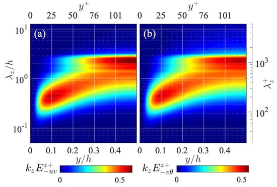
Figure 4.
Spanwise one-dimensional spectra of (a) the Reynolds shear stress and (b) turbulent heat transfer , presented in the same manner as in Figure 3.
3.2. Interscale Fluxes of the Reynolds Stresses and Temperature-Related Statistics
Next, the interscale fluxes of the temperature-related spectra are investigated. Figure 5 presents the distributions of the spanwise interscale flux of the streamwise turbulent energy , temperature fluctuation , and temperature-velocity correlation . Here, as can be seen from Equations (8) and (9), the positive values indicate forward energy fluxes (i.e., from larger to smaller scales) in the spanwise length-scale direction, whereas the negative values represent the inverse (from smaller to larger scales) energy fluxes. As shown in Figure 5a, the turbulent energy flux indicates mainly forward interscale energy transfers from larger to smaller in the relatively small range throughout the channel, but it also presents backward energy fluxes from smaller to larger in a relatively large range in the near-wall region. It is interesting to note that such inverse interscale energy transfer is not observed in the streamwise length-scale direction [4,7], and the corresponding physical phenomenon has still not been elucidated.
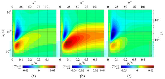
Figure 5.
Space-wavelength () diagrams of spanwise interscale fluxes of (a) the turbulent kinetic energy , (b) temperature fluctuation , and (c) temperature-velocity correlation . The values are scaled by , , , and , respectively.
As shown in Figure 5b, the spanwise interscale flux of the temperature fluctuation presents a qualitatively similar distribution to the streamwise turbulent energy flux , presenting a region of backward interscale energy transfers at relatively large in the near-wall region and forward interscale energy fluxes at smaller throughout the channel. One can, however, also observe in the distribution of that the region of backward energy flux somewhat shrinks, and instead, the magnitude of the forward energy flux around the channel centre is relatively stronger than .
Figure 5c shows the distribution of the spanwise interscale flux of the velocity-temperature correlation . One can observe that also has a qualitatively similar distribution to those of the turbulent energy flux and the temperature fluctuation flux , presenting both a backward and forward energy flux. Furthermore, as compared to the distributions of and , the region of backward energy flux is relatively large and the peak magnitude of the forward energy flux at small near the wall is relatively small.
The spanwise interscale fluxes of the Reynolds shear stress and the turbulent heat flux are also presented in Figure 6. As shown in the panel (a), the Reynolds shear stress flux indicates, interestingly, the backward transfers throughout the channel, as first experimentally observed by Kawata and Alfredsson [1]. This is in contrast to the turbulent energy transfer , which mainly indicates forward transfers throughout the channel except for the near-wall region. Such inverse interscale transport of the Reynolds shear stress has also been reported in turbulent channel [11] and boundary-layer [5] flows.
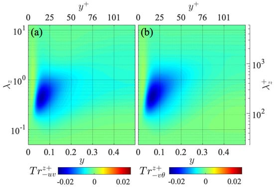
Figure 6.
Spanwise interscale fluxes of (a) Reynolds shear stress and (b) turbulent heat flux , presented in the same manner as in Figure 5.
The interscale transfer of the turbulent heat flux gives a similar distribution to that of , as presented in Figure 6b. The difference between the distributions of these spanwise interscale fluxes is that spans to slightly larger spanwise wavelengths than . While it is still unclear what physical phenomenon is represented by such an inverse interscale transfer of and , the similar distributions of and indicate a close analogy between the transport of the Reynolds shear stress and turbulent heat flux.
3.3. Spectra of Spatial Turbulent Fluxes of the Reynolds Stresses and Temperature-Related Statistics
We focus on the spatial turbulent transport of the Reynolds stresses and temperature-related statistics. Figure 7 presents the profiles of the triple velocity correlations and and those of the triple velocity-temperature correlations and . As for the physical interpretations of these third-order statistics, and represent, respectively, the wall-normal spatial fluxes of the velocity fluctuation and the temperature fluctuation , which are caused by turbulent fluid motions. Similarly, and indicate the turbulent spatial fluxes of the Reynolds shear stress and the turbulent heat transfer , respectively. As discussed in Section 2.2, these third-order statistics represent the spatial transport effect caused by interactions between different scales. As shown in Figure 7, the profiles of the triple correlations are all qualitatively similar, indicating transport further towards the wall in the near-wall region and transport towards the channel centre in the far-wall region.
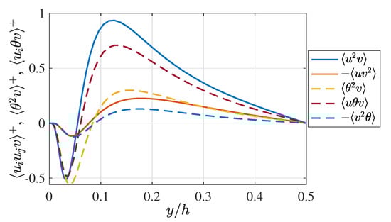
Figure 7.
Profiles of the velocity triple correlations and and the temperature-velocity triple correlations and . The values are scaled by , , or .
Figure 8 presents the distributions of the spanwise one-dimensional spectra of the turbulent energy transports , , and in the premultiplied form. These spectra represent the spectral contents of the triple correlations , , and presented in Figure 7. As shown in Figure 8, these spectra of spatial energy fluxes show similar distributions, indicating that the negative (i.e., towards the wall) spatial transport in the near-wall region mainly occurs at the largest wavelength , while the positive (towards the channel centre) transport occurs at two smaller scales: the middle scale roughly at and relatively small wavelengths around (). As the wavelength of the negative peak at the largest scale coincides with the typical spanwise spacing of u-streaks of the very-large-scale structure, the large-scale negative peak presumably represents the turbulence transports in which the fluctuating velocities and temperature are carried towards the wall vicinity by the secondary fluid motions of the very-large-scale structures. As for the positive peak at a relatively small scale , this wavelength fairly matches the peak location of the premultiplied wall-normal turbulent energy spectrum in the near-wall region [27], which is likely related to the coherent fluid motions in the near-wall region. Therefore, it can be inferred that this positive peak indicates the turbulent energy transport driven by the wall-normal fluid motions by the near-wall coherent structures. On the other hand, the wavelength of the positive peak on the larger-scale side, (), is on the order of the full channel height h, but any corresponding characteristic length scale of coherent fluid motion is not found. As this scale lies in the middle wavelength range between the length scales of the very-large-scale and near-wall structures, this positive peak may represent the energy transport caused by interactions between these inner and outer coherent structures.
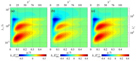
Figure 8.
Spanwise one-dimensional premultiplied spectra of turbulent spatial fluxes of (a) streamwise turbulent energy , (b) temperature fluctuation , and (c) temperature-velocity correlation , presented in the same manner as in Figure 3. The values are scaled by , , and , respectively.
Figure 9 presents the distributions of the spatial flux spectra of the Reynolds shear stress and the turbulent heat transfer . Similarly to other spatial flux spectra presented in Figure 8, and are the spectral contents of the triple correlations and presented in Figure 7, indicating the wall-normal fluxes of the Reynolds shear stress and the turbulent heat flux at each wavelength , respectively. As shown in the figure, these spatial flux spectra of the cross correlations present qualitatively similar distributions to those of the spatial turbulent energy fluxes, such as and presented in Figure 8, indicating the peak of negative transport at the largest wavelength near the wall, and the positive transport peaks at two smaller wavelengths in the relatively far-wall region. This tendency is in contrast to the interscale fluxes in that the interscale fluxes of the cross correlations and show clearly different behaviours from those of turbulent energies such as and , as observed in Figure 5 and Figure 6.
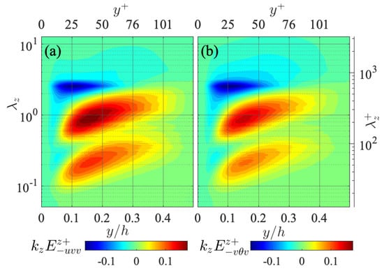
Figure 9.
Spanwise one-dimensional premultiplied spectra of turbulent spatial fluxes of (a) Reynolds shear stress and (b) the turbulent heat flux , presented in the same manner as in Figure 3. The values are scaled by and , respectively.
As described so far, the spectral distributions of the fluctuating velocity and temperature fields have been investigated with respect to their interscale and spatial fluxes, and it has been observed that the temperature-related statistics essentially show similar distributions to the corresponding turbulence statistics, indicating a close similarity between the fluctuating velocity and temperature fields. In the next section, the spectral budgets of the transport equations of the temperature-related statistics are investigated further in detail.
3.4. Budget Analysis of Spectral Transport Equations
Now, we investigate the transport budget of the temperature-related spectra , , and in detail. The transport budgets of the Reynolds stress spectra are also given in Appendix A and compared to these temperature-related spectra transport when necessary for discussion. Figure 10 presents the distributions of terms in the transport equation of the temperature fluctuation spectrum :
As shown in the top-left panel, the temperature fluctuation is produced by mainly at a relatively small wavelength of in the near-wall region, which roughly corresponds to the y-position and the spanwise length scale of the coherent structure in the near-wall region. This tendency is quite similar to the distribution of the streamwise turbulent energy production spectrum given in Figure A1, see Appendix A. The similarity between these productions can be understood by noting that and depend on the cospectra and , respectively, as
and the distributions of and and the profiles of U and are similar to each other, respectively, as presented in Figure 1 and Figure 4.
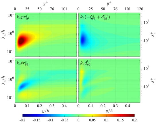
Figure 10.
Space-wavelength () diagrams of terms in the transport equation of the temperature fluctuation spectrum : (top left) production ; (top right) viscous terms ; (bottom left) interscale transport ; (bottom right) turbulent diffusion . The terms are presented in the premultiplied form, and the values are scaled by .
The distribution of the interscale transport presents the consequential energy gain/loss by the interscale energy flux shown in Figure 5 as , and it is shown in Figure 10 that the energy is removed from the region around the peak of and transported towards both larger and smaller ranges in the near-wall region by the interscale energy transport , while in the channel-core region, the energy is mainly transported in the forward direction from around to a smaller range.
The distribution of the spectral turbulent diffusion represents the energy gain/loss by the turbulent spatial flux presented in Figure 8, as . Its contribution is relatively small as compared to the other terms, but it can be seen that the energy is supplied to the wall vicinity at a large wavelength , and the energy transport towards the channel central region is also observed at two relatively small wavelength ranges, corresponding to the distribution of the turbulent spatial flux . The energy produced by and transported by and is eventually dissipated by the viscous dissipation . Such distributions of the terms in the transport equation described above are quite similar to those of the corresponding terms in the transport equation given in Figure A1.
The clear difference between the transport equations of the temperature fluctuation spectrum and the streamwise turbulent energy is that no pressure-related term exists in the transport equation, whereas in the transport, the pressure-strain cospectrum plays an important role in redistributing energy from to other components of turbulent energy spectra. Despite such a distinct difference, the distributions of the terms in the equation are quite similar to those of the corresponding terms of the transport equation (compare Figure 10 and Figure A1). In the following, the budget balances of the and equations are compared in more detail.
Figure 11 presents a detailed balance between the terms of the and equations at a near-wall location and the quarter height of the channel (). The values are scaled by the maximum value of each production term. As shown in the panel (a), the profiles of the production, interscale transport, and turbulent diffusion of the and transport equations show a good collapse in the near-wall region. The production terms indicate a significant energy gain at , as already pointed out above, and the interscale transport terms are shown to transfer the energy from this energy-producing wavelength to both larger and smaller ranges, where the turbulent diffusion terms transfer some energy to other y-positions. As previously mentioned, there is no term in the transport budget corresponding to the pressure-strain term in the transport, and the consequential difference between the budget balances of the and transport equation is mainly manifested by the viscous terms. As there is no energy absorption by the pressure-strain cospectrum in the budget, the viscous terms show a clearly larger contribution than to compensate for the absence of the pressure term and, thus, the transport equation is balanced.
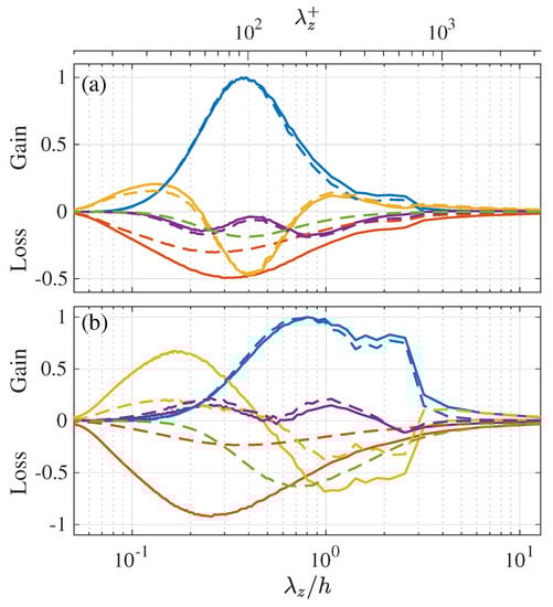
Figure 11.
Detailed budget balance of the and transport equation at (a) a near-wall location and (b) the quarter height of the channel : (blue) production; (red) viscous dissipation+viscous diffusion; (yellow) interscale transport; (purple) turbulent diffusion; (light green) pressure-strain cospectrum . The solid and dashed lines represent terms in the and equations, respectively. The terms are given in the premultiplied form, and the values are scaled by the peak value of each production term.
At the quarter height of the channel , as shown in Figure 11b, the profiles of the production terms collapse similarly to those in the near-wall region, but the range where energy is dissipated by viscosity is significantly smaller than the energy-producing range. Hence, the interscale transport terms bridge these energy-producing and -dissipating ranges by forward energy transfer and do not exhibit reversed energy transfer, unlike in the near-wall region. It is also observed that the production terms present not only the largest peak of energy gain at but also a secondary peak at , which corresponds to the very-large-scale structures. The turbulent diffusion terms present energy gains at two wavelength ranges, which represents energy supply from the near-wall region (see the and distributions in Figure 10 and Figure A1). The contribution of the pressure-strain correlation in the transport equation is relatively large compared to that in the near-wall location shown in the panel (a), and the interscale transport as well as the viscous terms show significantly larger contributions than the counterparts in the equation to compensate for the absence of the energy absorption by . Thus, both in the near- and far-wall regions of the channel, the energy productions in the and transports are quite similar to each other, but more energy is dissipated by the viscous terms in the transport, compensating for the absence of the energy loss by the pressure-related term.
The transport equation of the velocity-temperature cospectrum is written as
and the distributions of the terms in the right-hand side are presented in Figure 12. It is clearly seen here that the transport equation has a pressure term and it essentially functions as an energy sink throughout the channel, similarly to the pressure-strain energy redistribution term in the transport equation. It is also noteworthy that the production of the velocity-temperature cospectrum depends on both the Reynolds shear stress spectra and the turbulent heat flux spectra as
unlike the productions of other spectra, such as and , which only depend on either or . The distribution of is, however, similar to those of and , as the distributions of and are similar to each other and so are the profiles of U and . Each term of the transport equation presented in Figure 12 shows a similar distribution to the corresponding term in the transport equation shown in Figure A1. Since the transport equation has a pressure-related term, unlike the equation, the budget balance is even closer to the transport of the streamwise turbulent energy than that of the transport.
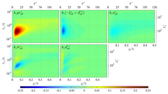
Figure 12.
Distribution of terms in the transport equation of the velocity-temperature cospectrum presented in the same manner as in Figure 10: (top left) production ; (top centre) viscous terms ; (top right) pressure term ; (bottom right) interscale transport ; (bottom centre) turbulent diffusion . The terms are presented in the premultiplied form, and the values are scaled by .
Now, we shed light on the transport of the turbulent heat flux spectrum . The transport equation of is written as
and the distributions of the terms on the right-hand side are presented in Figure 13. As shown here, is produced by the production term mainly in the near-wall region at wavelengths around , similarly to the other energy spectra and . The energy gain by the production is mainly balanced by the pressure term , and the viscous terms do not play an important role.
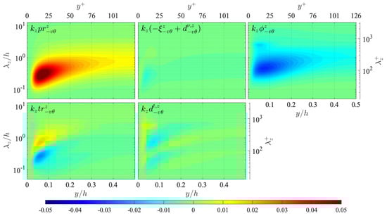
Figure 13.
Distribution of terms in the transport equation of the turbulent heat flux spectrum presented in the same manner as in Figure 12: (top left) production ; (top centre) viscous terms ; (top right) pressure term ; (bottom left) interscale transport ; (bottom centre) turbulent diffusion . The terms are presented in the premultiplied form, and the values are scaled by .
The turbulent transport terms and are shown to partly transport in scale and space, respectively. The interscale transport presents the energy gain/loss by the inverse interscale flux investigated in Figure 6, and the distribution shows that the turbulent heat flux is mainly transported from wavelengths around () to a larger range around () in the near-wall region. The distribution of indicates weak spatial transports similarly to and , where is supplied to the wall vicinity from the channel-core region at the largest wavelengths , and at a smaller range, is transported from the near- to far-wall region at two different wavelengths.
The tendencies of the terms in the transport equation described above are quite similar to those of the corresponding terms in the transport equation of the Reynolds shear stress spectrum , as can be seen by comparing Figure 13 in Figure A4 in Appendix A. It is particularly noteworthy here that the productions of and are both dependent on the wall-normal turbulent energy spectrum as
which indicates that the Reynolds shear stress and the turbulent heat flux are produced at the same scale.
Figure 14 presents a detailed comparison of the transport budgets of and at a near-wall location and the quarter height of the channel in the same manner as in Figure 11. Note here that in both panels the profiles of the productions and are exactly on top of each other since their profiles are similar, as shown by Equation (43). As shown here, at both wall-normal locations, the spectral budget balances of the and transport are quite similar to each other. It is also shown at both wall-normal locations that the peaks of the pressure terms are located at a larger than those of the production terms in both and transport, which indicates that the turbulent heat flux and the Reynolds shear stress are dissipated by the effect of pressure at larger spanwise wavelengths than those at which they are produced by the mean temperature or velocity gradients. Such tendencies are in contrast to the transport of the energy spectra such as and , where the energy is dissipated basically at smaller scales than produced. This is attributable to the contribution of the interscale transport terms and to transport the energy from smaller to larger scales.
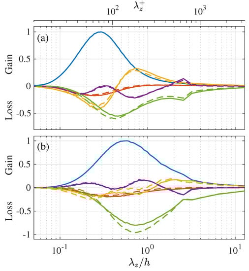
Figure 14.
Detailed budget balance of the and transport equation at (a) a near-wall location and (b) the quarter height of the channel presented in the same manner as in Figure 11: (blue) production; (red) viscous dissipation+viscous diffusion; (yellow) interscale transport; (purple) turbulent diffusion; (light green) pressure term.
It is interesting to note that the agreements between the turbulent diffusion terms and are particularly good, while a slight difference can be found between the interscale transport terms and , although both the turbulent diffusion and interscale transport represent the transport effect caused by nonlinear interactions between different scales. Such good agreement between the turbulent diffusion terms are also observed between the and transports, as already pointed out in Figure 11.
4. Discussion and Concluding Remarks
In the previous section, the spectral budgets of the temperature-related spectra, such as , , and , were compared with those of the corresponding Reynolds stress spectra, and , and a close analogy between those turbulence transports was indicated. Of particular interest is the close similarity between the spectral transports of the Reynolds shear stress and the turbulent heat flux , where inverse interscale transport from a smaller to larger is observed.
The turbulent diffusion and interscale transport are two different aspects of nonlinear multi-scale interactions of turbulence, and the physical phenomena these spatial and interscale transport terms represent is of great interest. As shown in Figure 14a, the turbulent diffusions and are shown to remove energy from the near-wall location in two ranges around and 180, and the removed and are partly transported towards the central region of the channel, as indicated by the profiles of and at given in Figure 14b. In particular, the energy gains by and at are shown to balance well with the energy loss by the interscale energy transport and , which suggests that the energy ( and ) spatially transferred from the near-wall region to this wall-normal location at relatively small is further transferred to a larger range. Kawata and Alfredsson [1] experimentally observed similar Reynolds shear stress transport from smaller near the wall to larger in the channel-core region in turbulent plane Couette flow and conjectured that it may represent the influences of the near-wall smaller-scale coherent structures on the very-large-scale structures, which is similar to the concept of a co-supporting cycle of the inner and outer structures proposed by Toh and Itano [34].
It should be mentioned here that the inverse interscale transport of the Reynolds shear stress and turbulent heat flux described so far are observed based on one-dimensional spanwise-Fourier-mode analysis, and therefore, the interscale energy transfer in the streamwise length scales is not investigated. In fact, such reversed interscale transfers are not observed by the analysis based on the streamwise Fourier modes. In a numerical simulation by Kawata and Tsukahara [4], spectral budget analysis was performed based on both one-dimensional streamwise and spanwise Fourier modes, and it was shown that the interscale transfers of the turbulent energy and Reynolds shear stress in the streamwise wavenumber direction are basically forward transfers (i.e., from larger to smaller scales). Lee and Moser [7] performed two-dimensional Fourier-mode analysis on the turbulent energy transport and showed that the energy transport between wavenumbers with the same magnitude but different directions, which may not represent energy transfer between really different length scales, can be observed as inverse interscale energy transfers through one-dimensional Fourier mode analysis. These observations suggest that the inverse energy transfers in the spanwise length scales may not simply be interpreted as interaction from smaller- to larger-scale structures.
Some recent studies, on the other hand, investigated the relationship between the inner-outer interaction in wall turbulence and the inverse interscale energy transfers in the spanwise length scales in detail. Doohan et al. [3] investigated the interactions between self-sustaining processes (SSPs) of coherent structures near and away from the wall and argued that the energy transfer from the smaller-scale SSP leads to the formation of the wall-reaching part of streaks of the larger-scale SSP. Chiarini et al. [11] also investigated spatial and interscale energy fluxes by analysing the anisotropic generalised Kolmogorov equation taking into account both the streamwise and spanwise length scale and observed some energy paths from smaller scales near the wall to larger scales away from the wall. Chan et al. [5] also observed the inverse interscale transport of the Reynolds shear stress in a turbulent boundary layer, and based on a detailed quadrant analysis, they interpreted it as the net energy transfer from the small-scale ejection (Q2) and sweep (Q4) events to their large-scale counterparts. Thus, what the inverse interscale energy transports in the spanwise lengths scales is still a subject of intense debate. Nevertheless, the transport of the turbulent heat flux spectrum is found to be quite similar to that of the Reynolds shear stress spectrum , which indicates a close scale-by-scale similarity between the turbulent momentum and heat transfers.
In the present study, the transport budgets of temperature-related spectra, such as the temperature-variance and turbulent heat flux spectra, were investigated in turbulent plane Couette flow with a passive-scalar heat transfer at the Reynolds number and the Prandtl number based on DNS data. It was found that the transport budgets of the temperature-related spectra present quite similar tendencies to those of the corresponding Reynolds stress spectra, including the spectral transport of the Reynolds shear stress and turbulent heat flux, where inverse interscale transfers are observed throughout the channel. It is also noteworthy that the distributions of the spatial flux spectra are all similar, regardless of the spatial fluxes of turbulent energies such as and or those of cross correlations such as and . This is in contrast to how the interscale fluxes of and exhibit notably different behaviours from those of turbulent energies such as and . Our next task is to elucidate what physical phenomena these spatial and interscale turbulence transport represent. The present investigation is limited to single values of the Reynolds and Prandtl number, and therefore, the Reynolds- and Prandtl-number dependency of these interscale and spatial fluxes should also be investigated in future studies.
Author Contributions
Conceptualization, methodology, data analysis, writing—original draft preparation, funding acquisition, T.K.; writing—review and editing, supervision, T.T. All authors have read and agreed to the published version of the manuscript.
Funding
This work was supported by the Japan Society for the Promotion of Science (JSPS) through JSPS KAKENHI, Grant No. JP20K14654. The numerical simulations in the present study were performed by SX-ACE supercomputers at the Cybermedia Center of Osaka University.
Institutional Review Board Statement
Not applicable.
Informed Consent Statement
Not applicable.
Data Availability Statement
The data that support the findings of this study are available from the corresponding author upon reasonable request.
Conflicts of Interest
The authors declare no conflict of interest.
Nomenclature
| Spanwise one-dimensional spectra of | |
| Spanwise one-dimensional spectra of | |
| , , , , , , | Spanwise one-dimensional spectra of , , |
| , , , , and | |
| Spanwise one-dimensional spectra of | |
| Spanwise one-dimensional spectra of | |
| , , , , | Spanwise one-dimensional spectra of turbulent spatial |
| fluxes , , , , and | |
| h | Full channel height |
| Spanwise wavenumber | |
| Cutoff spanwise wavenumber for large- and | |
| small-scale decomposition | |
| , | Streamwise and spanwise lengths of computational |
| domain | |
| p | Pressure fluctuation |
| Prandtl number defined as | |
| Reynolds number defined as | |
| Friction Reynolds number defined as | |
| , | Temperature of top and bottom wall |
| Temperature difference between top and bottom wall, | |
| Friction temperature defined as , where | |
| and are mean wall heat flux and fluid specific | |
| heat at constant pressure, respectively | |
| Interscale flux of in spanwise length scales | |
| , , , , | Interscale flux of , , , , in |
| spanwise length scales | |
| U | Mean streamwise velocity |
| Translating speed of top wall | |
| u, v, w | Fluctuation of streamwise, wall-normal, and spanwise |
| velocity components | |
| Fluctuation of velocity component in direction | |
| Friction velocity defined as , where is | |
| mean wall shear stress | |
| x, y, z | Axes of the coordinates in the streamwise, wall-normal, |
| and spanwise directions | |
| Thermal diffusivity of fluid | |
| Half channel height, i.e., | |
| Kinematic viscosity of fluid | |
| Density of fluid |
| , | Mean temperature and temperature fluctuation |
| spanwise wavelength, i.e., | |
| ⟨⟩ | Averaged quantities |
| Terms in transport equations | |
| , , , , | Production, viscous dissipation, pressure-gradient, |
| viscous diffusion, and turbulent spatial transport | |
| terms in transport equation | |
| , | Pressure-strain correlation and pressure diffusion |
| terms in transport equation | |
| , , , | Production, viscous dissipation, viscous diffusion, and |
| turbulent spatial transport terms in transport | |
| equation | |
| , , , , | Production, viscous dissipation, pressure-gradient, |
| viscous diffusion, and turbulent spatial transport terms | |
| in transport equation | |
| , , , , , | Production, viscous dissipation, pressure-gradient, |
| viscous diffusion, turbulent spatial transport, and | |
| interscale transport terms in transport equation | |
| , | Pressure-strain and pressure transport terms in |
| transport equation | |
| , , , , | Production, viscous dissipation, viscous diffusion, |
| turbulent spatial transport, and interscale transport | |
| terms in transport equation | |
| , , , , , | Production, viscous dissipation, pressure-gradient, |
| viscous diffusion, turbulent spatial transport, and | |
| interscale transport terms in transport equation | |
| , , , , , | Production, viscous dissipation, pressure-gradient, |
| viscous diffusion, turbulent spatial transport, and | |
| interscale transport terms in transport equation | |
| , , , , , | Production, viscous dissipation, pressure-gradient, |
| viscous diffusion, turbulent spatial transport, and | |
| interscale transport terms in transport equation | |
| , , , , , | Production, viscous dissipation, pressure-strain, |
| viscous diffusion, turbulent spatial transport, and | |
| interscale transport terms in transport equation | |
| , , , , , | Pressure-strain, viscous dissipation, pressure transport, |
| viscous diffusion, turbulent spatial transport, and | |
| interscale transport terms in transport equation | |
| , , , , | Pressure-strain, viscous dissipation, viscous diffusion, |
| turbulent spatial transport, and interscale transport | |
| terms in transport equation | |
| , , , , , | Production, viscous dissipation, pressure-gradient, |
| viscous diffusion, turbulent spatial transport, and | |
| interscale transport terms in transport equation | |
| Superscripts | |
| L, S | Large- and small-scale part |
| + | Scaled viscous units, based on , , |
Appendix A. Spectral Budgets of the Reynolds Stress Transports
Here, the transport budgets of the Reynolds stress spectra are presented for comparison to those of the temperature-related spectra given in Figure 10, Figure 11, Figure 12, Figure 13 and Figure 14. The transport equations of the streamwise turbulent energy , wall-normal turbulent energy , and spanwise turbulent energy are, respectively, written as
and the distributions of each term on the right-hand side of these transport equations are given in Figure A1, Figure A2 and Figure A3. Among the turbulent energy spectra, only the streamwise component has energy production from the mean flow, and the energy sources for the wall-normal and spanwise components and are the energy redistribution by the pressure-strain cospectra and , respectively. Note here that
at any y-location and any wavelength .
The transport equation of the Reynolds shear stress spectrum is
and the distributions of the budget terms are shown in Figure A4.
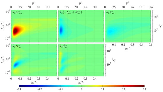
Figure A1.
Distribution of terms in the transport equation of the streamwise turbulent energy spectrum , presented in the same manner as in Figure 12: (top left) production ; (top centre) viscous terms ; (top right) pressure-strain energy redistribution ; (bottom left) interscale transport ; (bottom centre) turbulent diffusion . The terms are presented in the premultiplied form, and the values are scaled by .
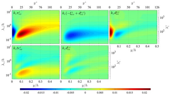
Figure A2.
Distribution of terms in the transport equation of the wall-normal turbulent energy spectrum , presented in the same manner as in Figure 12: (top left) pressure-strain energy redistribution ; (top centre) viscous terms ; (top right) pressure diffusion ; (bottom left) interscale transport ; (bottom right) turbulent diffusion . The terms are presented in the premultiplied form, and the values are scaled by .
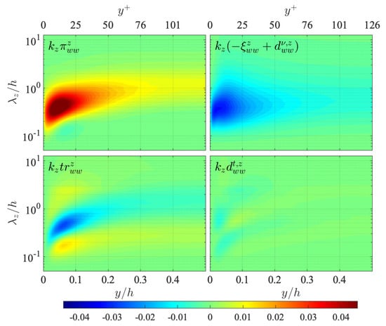
Figure A3.
Distribution of terms in the transport equation of the spanwise turbulent energy spectrum , presented in the same manner as in Figure 12: (top left) pressure-strain energy redistribution ; (top right) viscous terms ; (bottom left) interscale transport ; (bottom right) turbulent diffusion . The terms are presented in the premultiplied form, and the values are scaled by .
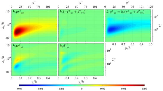
Figure A4.
Distribution of terms in the transport equation of the Reynolds shear stress spectrum , presented in the same manner as in Figure 12: (top left) production ; (top centre) viscous terms ; (top right) pressure term ; (bottom left) interscale transport ; (bottom centre) turbulent diffusion . The terms are presented in the premultiplied form, and the values are scaled by .
References
- Kawata, T.; Alfredsson, P.H. Inverse Interscale Transport of the Reynolds shear stress in plane Couette turbulence. Phys. Rev. Lett. 2018, 120, 244501. [Google Scholar] [CrossRef]
- Wang, W.; Pan, C.; Wang, J. Energy transfer structures associated with large-scale motions in a turbulent boundary layer. J. Fluid Mech. 2020, 906, A14. [Google Scholar] [CrossRef]
- Doohan, P.; Wills, A.P.; Hwang, Y. Minimal multi-scale dynamics of near-wall turbulence. J. Fluid Mech. 2021, 913, A8. [Google Scholar] [CrossRef]
- Kawata, T.; Tsukahara, T. Scale interactions in turbulent plane Couette flows in minimal domains. J. Fluid Mech. 2021, 911. [Google Scholar] [CrossRef]
- Chan, C.; Schlatter, P.; Chin, R. Interscale transport mechanisms in turbulent boundary layers. J. Fluid Mech. 2021, 921, A13. [Google Scholar] [CrossRef]
- Mizuno, Y. Spectra of energy transport in turbulent channel flows for moderate Reynolds numbers. J. Fluid Mech. 2016, 805, 171–187. [Google Scholar]
- Lee, M.; Moser, R.D. Spectral analysis of the budget equation in turbulent channel flows at high Reynolds number. J. Fluid Mech. 2019, 860, 886–938. [Google Scholar] [CrossRef] [Green Version]
- Wang, H.; Yang, Z.; Wu, T.; Wang, S. Coherent structures associated with interscale energy transfer in turbulent channel flows. Phys. Rev. Fluids 2021, 6, 104601. [Google Scholar] [CrossRef]
- Cimarelli, A.; De Angelis, E.; Casciola, C.M. Paths of energy in turbulent channel flows. J. Fluid Mech. 2013, 715, 436–451. [Google Scholar] [CrossRef]
- Cimarelli, A.; De Angelis, E.; Jiménez, J.; Casciola, C.M. Cascades and wall-normal fluxes in turbulent channel flows. J. Fluid Mech. 2016, 796, 417–436. [Google Scholar]
- Chiarini, A.; Mauriello, M.; Gatti, D.; Quadrio, M. Ascending-descending and direct-inverse cascades of Reynolds stresses in turbulent Couette flow. J. Fluid Mech. 2021, 930, A9. [Google Scholar] [CrossRef]
- Smits, A.; McKeon, B.; Marusic, I. High–Reynolds number wall turbulence. Annu. Rev. Fluid Mech. 2011, 43, 353–375. [Google Scholar] [CrossRef] [Green Version]
- Cho, M.; Hwang, Y.; Choi, H. Scale interactions and spectral energy transfer in turbulent channel flow. J. Fluid Mech. 2018, 854, 474–504. [Google Scholar] [CrossRef]
- Hamba, F. Turbulent energy density in scale space for inhomogeneous turbulence. J. Fluid Mech. 2018, 842, 532–553. [Google Scholar] [CrossRef]
- Kawamura, H.; Ohsaka, K.; Abe, H.; Yamamoto, K. DNS of turbulent heat transfer in channel flow with low to medium-high Prandtl number fluid. Int. J. Heat Fluid Flow 1998, 19, 482–491. [Google Scholar] [CrossRef]
- Kawamura, H.; Abe, H.; Matsuo, Y. DNS of turbulent heat transfer in channel flow with respect to Reynolds and Prandtl number effects. Int. J. Heat Fluid Flow 1999, 20, 196–207. [Google Scholar] [CrossRef]
- Hane, S.; Tsukahara, T.; Iwamoto, K.; Kawamura, H. DNS of turbulent heat transfer in plane Couette flow. In Proceedings of the International Heat Transfer Conference, Sydney, Australia, 13–18 August 2006. [Google Scholar] [CrossRef]
- Tsukahara, T.; Iwamoto, K.; Kawamura, H. On the large-scale structure of turbulent heat transfer in a plane Couette flow. Therm. Sci. Eng. 2007, 15, 151–161. (In Japanese) [Google Scholar]
- Antonia, R.A.; Abe, H. Analogy between velocity and scalar fields in a turbulent channel flow. J. Fluid Mech. 2009, 628, 241–268. [Google Scholar] [CrossRef]
- Abe, H.; Kawamura, H.; Toh, S.; Itano, T. Effect of the streamwise computational domain size on DNS of a turbulent channel flow at high Reynolds number. In Advances in Turbulence XI; Palma, J.M.L.M., Lopes, A.S., Eds.; Springer: Berlin/Heidelberg, Germany, 2007; pp. 233–235. [Google Scholar]
- Alcántara-Ávila, F.; Hoyas, S.; Pérez-Quiles, M.J. DNS of thermal channel flow up to Reτ=2000 for medium to low Prandtl numbers. Int. J. Heat Mss Transf. 2018, 127, 349–361. [Google Scholar] [CrossRef]
- Alcántara-Ávila, F.; Gandía-Barberá, S.; Hoyas, S. Evidences of persisting thermal structures in Couette flows. Int. J. Heat Fluid Flow 2019, 76, 287–295. [Google Scholar] [CrossRef]
- Alcántara-Ávila, F.; Hoyas, S.; Jezabel Pérez-Quiles, M. Direct numerical simulation of thermal channel flow for Reτ=5000 and Pr=0.71. J. Fluid Mech. 2021, 916, A29. [Google Scholar] [CrossRef]
- Alcántara-Ávila, F.; Hoyas, S. Direct numerical simulation of thermal channel flow for medium–high Prandtl numbers up to Reτ=2000. Int. J. Heat Mss Transf. 2021, 176, 1214112. [Google Scholar] [CrossRef]
- Komminaho, J.; Lundbladh, A.; Johansson, A.V. Very large structures in plane turbulent Couette flow. J. Fluid Mech. 1996, 320, 259–285. [Google Scholar] [CrossRef]
- Kitoh, O.; Nakabayashi, K.; Nishimura, F. Experimental study on mean velocity and turbulence characteristics of plane Couette flow: Low-Reynolds-number effects and large longitudinal vortical structure. J. Fluid Mech. 2005, 539, 199–227. [Google Scholar] [CrossRef]
- Tsukahara, T.; Kawamura, H.; Shingai, K. DNS of turbulent Couette flow with emphasis on the large-scale structure in the core region. J. Turbul. 2006, 7, N19. [Google Scholar] [CrossRef]
- Kitoh, O.; Umeki, M. Experimental study on large-scale streak structure in the core region of turbulent plane Couette flow. Phys. Fluids 2008, 20, 025107. [Google Scholar] [CrossRef]
- Avsarkisov, V.; Hoyas, S.; Oberlack, M.; García-Galache, J.P. Turbulent plane Couette flow at moderately high Reynolds number. J. Fluid Mech. 2015, 751, R1. [Google Scholar] [CrossRef]
- Orlandi, P.; Bernardini, M.; Pirozzoli, S. Poiseuille and Couette flows in the transitional and fully turbulent regime. J. Fluid Mech. 2015, 770, 424–441. [Google Scholar] [CrossRef]
- Lee, M.; Moser, R.D. Extreme-scale motions in turbulent plane Couette flows. J. Fluid Mech. 2018, 842, 128–145. [Google Scholar] [CrossRef] [Green Version]
- Kawata, T.; Tsukahara, T. Spectral analysis on dissimilarity between the turbulent heat and momentum transport in plane Couette turbulence. Phys. Fluids 2022. [Google Scholar] [CrossRef]
- Kawata, T.; Alfredsson, P.H. Scale interactions in turbulent rotating planar Couette flow: Insight through the Reynolds stress transport. J. Fluid Mech. 2019, 879, 255–295. [Google Scholar] [CrossRef]
- Toh, S.; Itano, T. Interaction between a large-scale structure and near-wall structures in channel flow. J. Fluid Mech. 2005, 524, 249–262. [Google Scholar] [CrossRef]
Publisher’s Note: MDPI stays neutral with regard to jurisdictional claims in published maps and institutional affiliations. |
© 2022 by the authors. Licensee MDPI, Basel, Switzerland. This article is an open access article distributed under the terms and conditions of the Creative Commons Attribution (CC BY) license (https://creativecommons.org/licenses/by/4.0/).