
A 1D Reduced-Order Model (ROM) for a Novel Latent Thermal Energy Storage System


Abstract
:1. Introduction
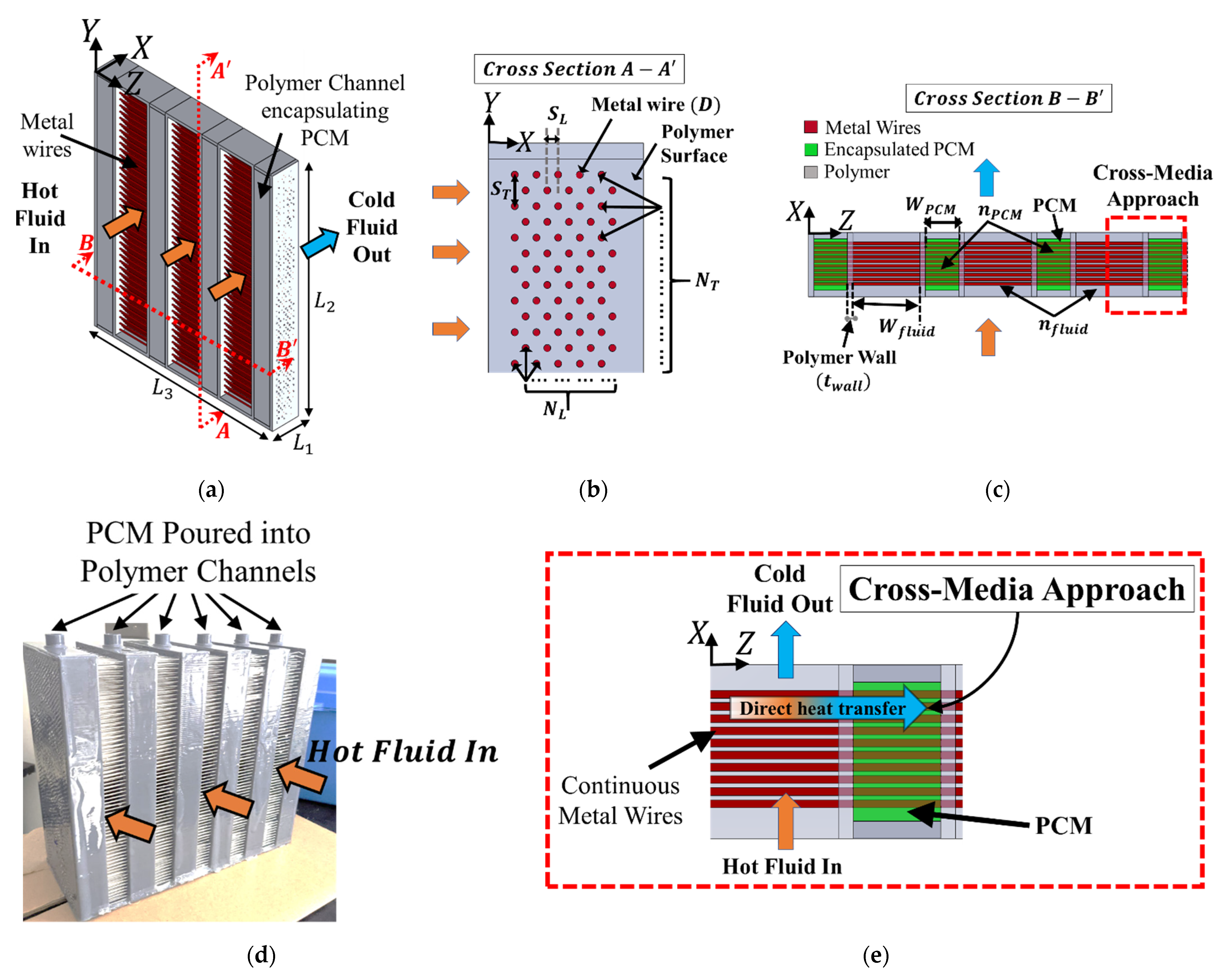
2. Design of a Novel TES System
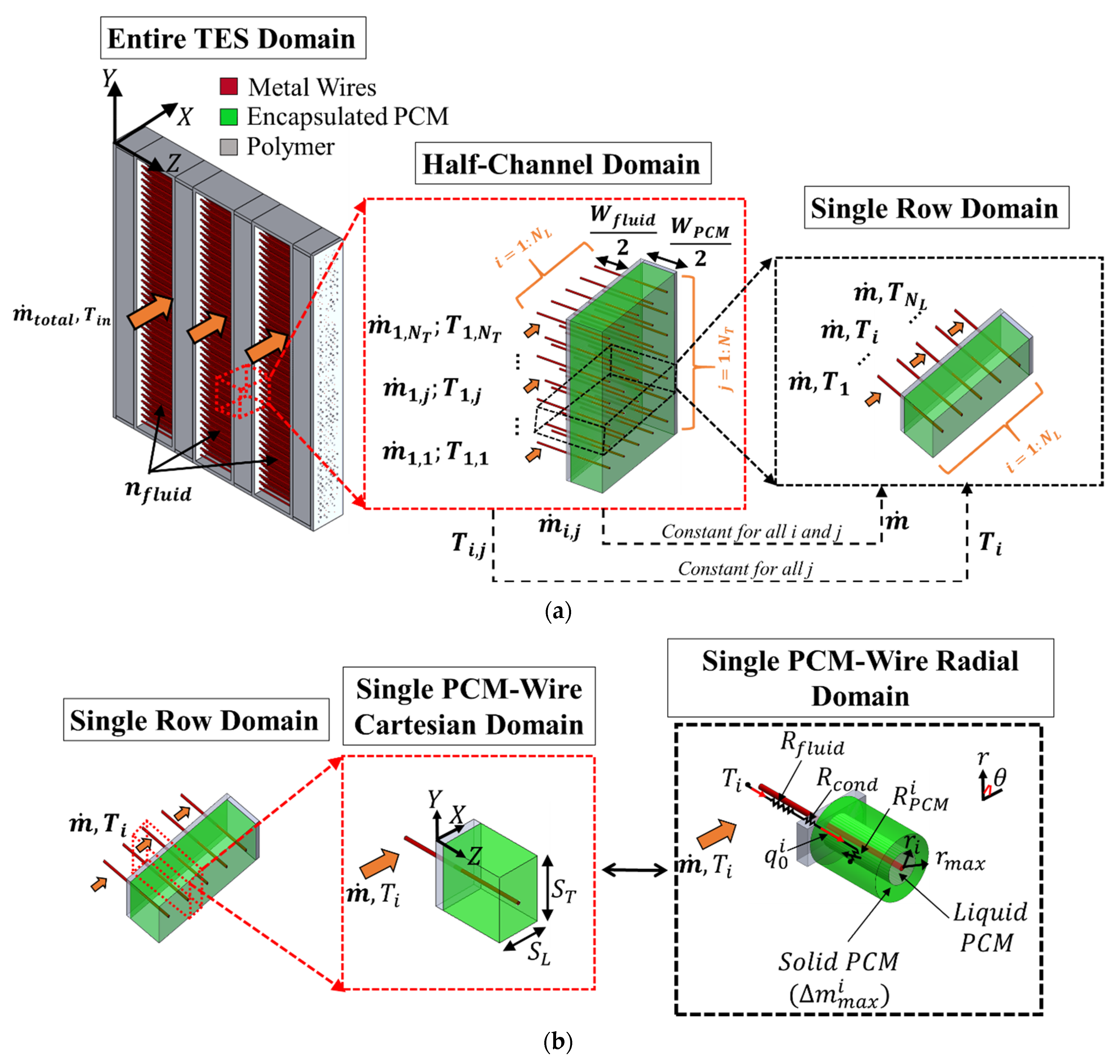
3. 1D ROM
3.1. Domain Simplifications and Assumptions
- Constant and isotropic material properties of fluid, polymer, metal, and PCM (both liquid and solid phases);
- Fully developed flow;
- No hysteresis in the melting temperature of the PCM ();
- Entire PCM at its melting temperature (), initially;
- Negligible effects of gravity;
- Heat transfer only through wire fins, and negligible conduction through polymer walls;
- Uniform mass flow rate () and temperature () profiles, per unit area at the inlet;
- 1D radial conduction in PCM;
- Quasi-steady-state approximation ( or negligible thermal capacitance of PCM. Here, .
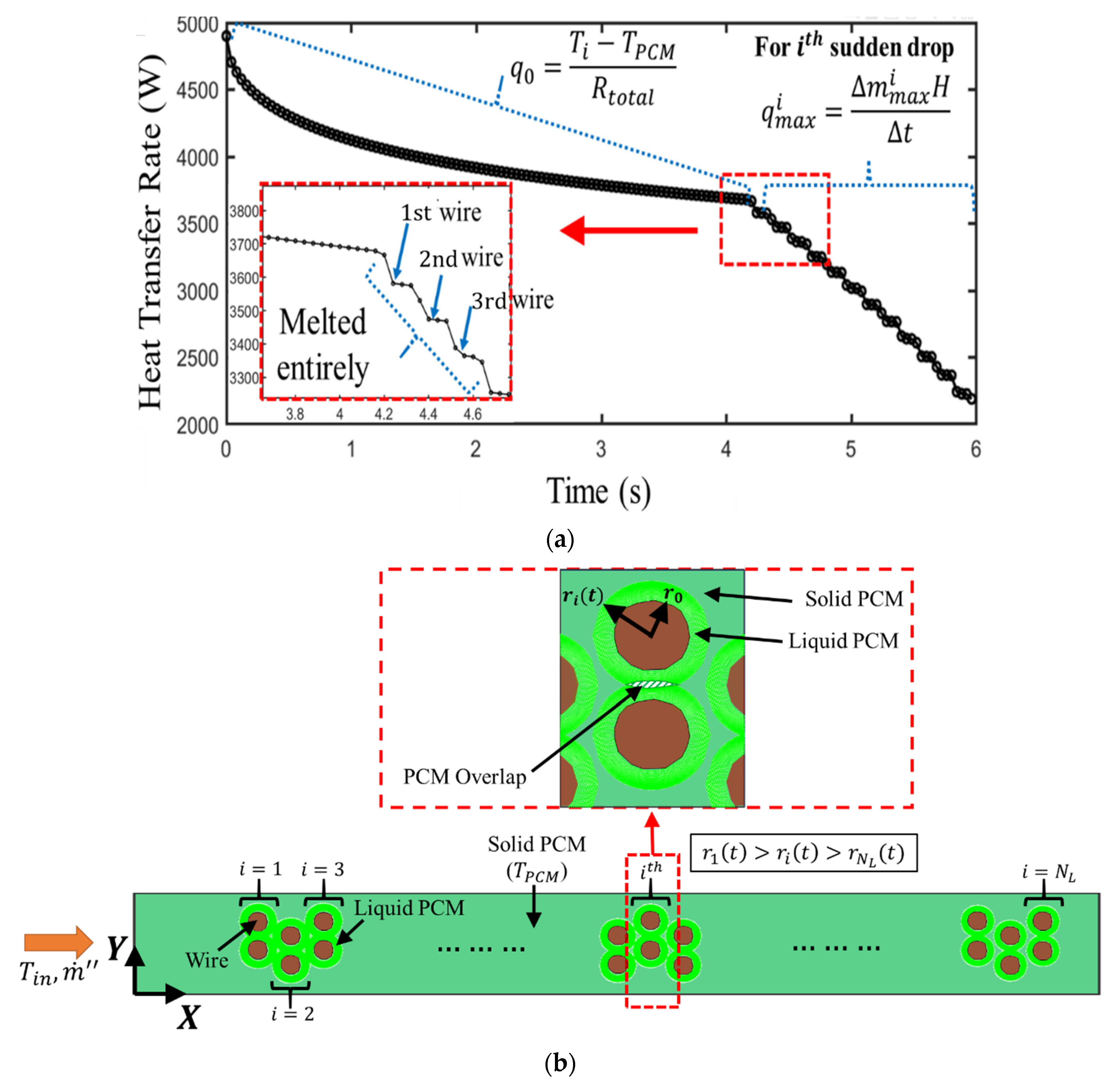
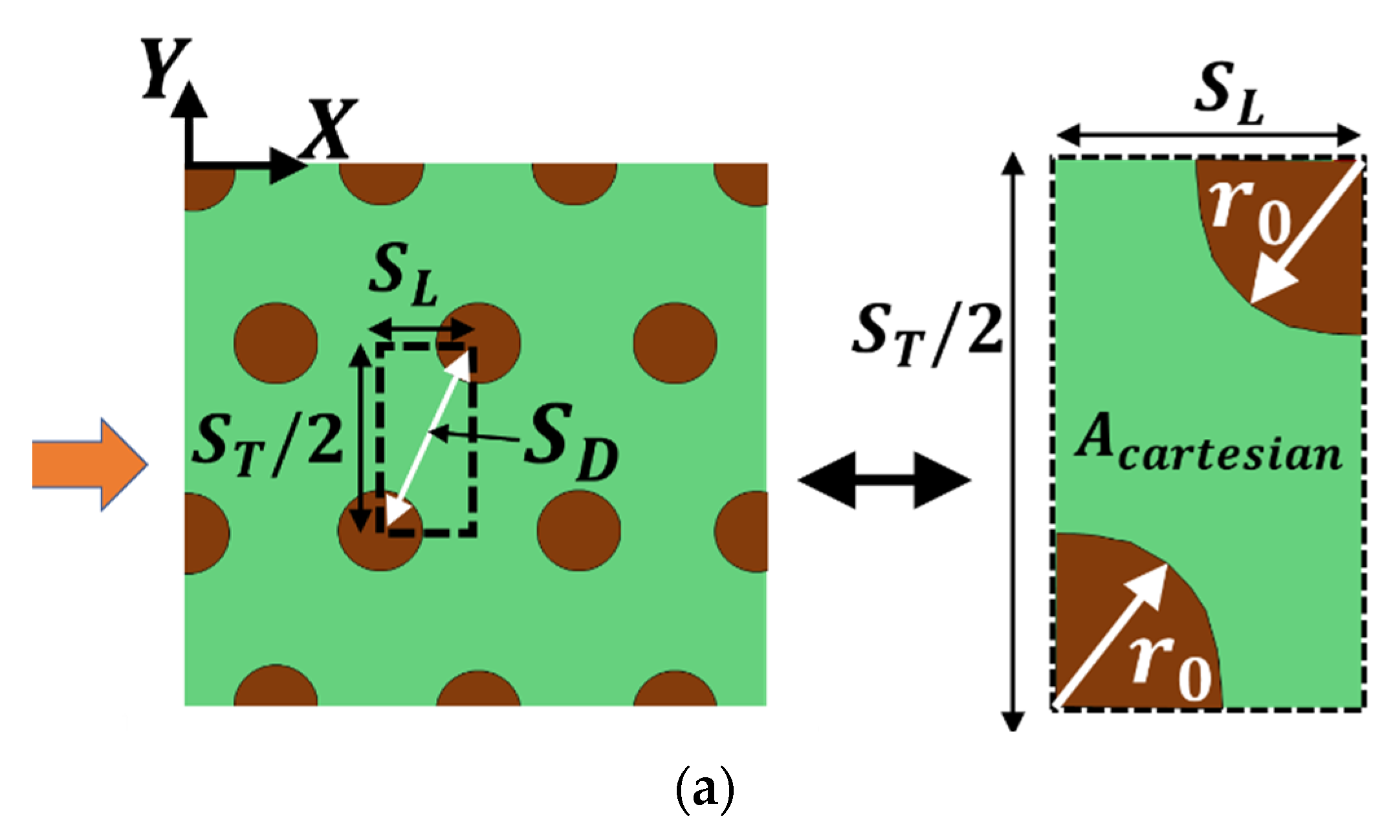
3.2. Domain Geometry of PCM-Wire Cylinders ()
3.3. Governing Equations
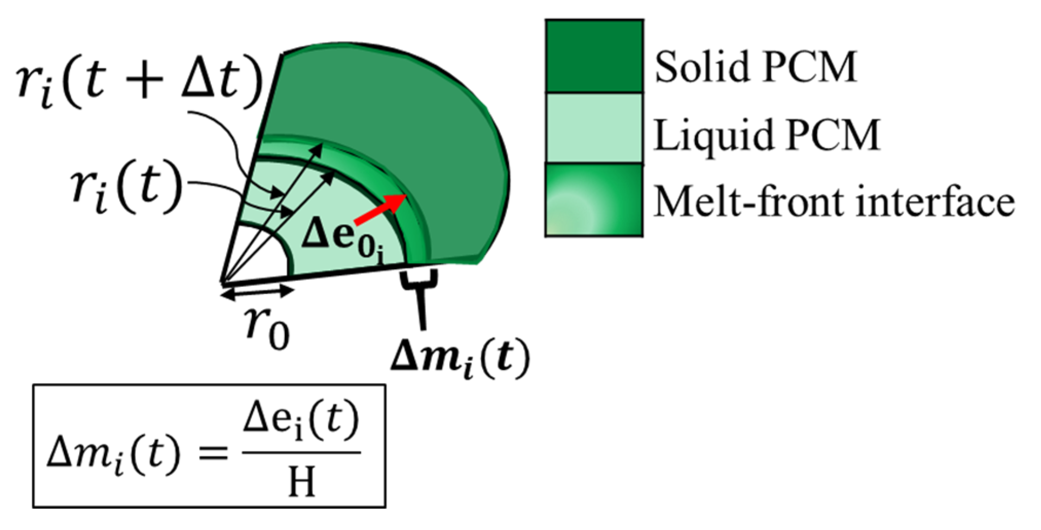
3.3.1. Latent Energy Stored in Single PCM-Wire,
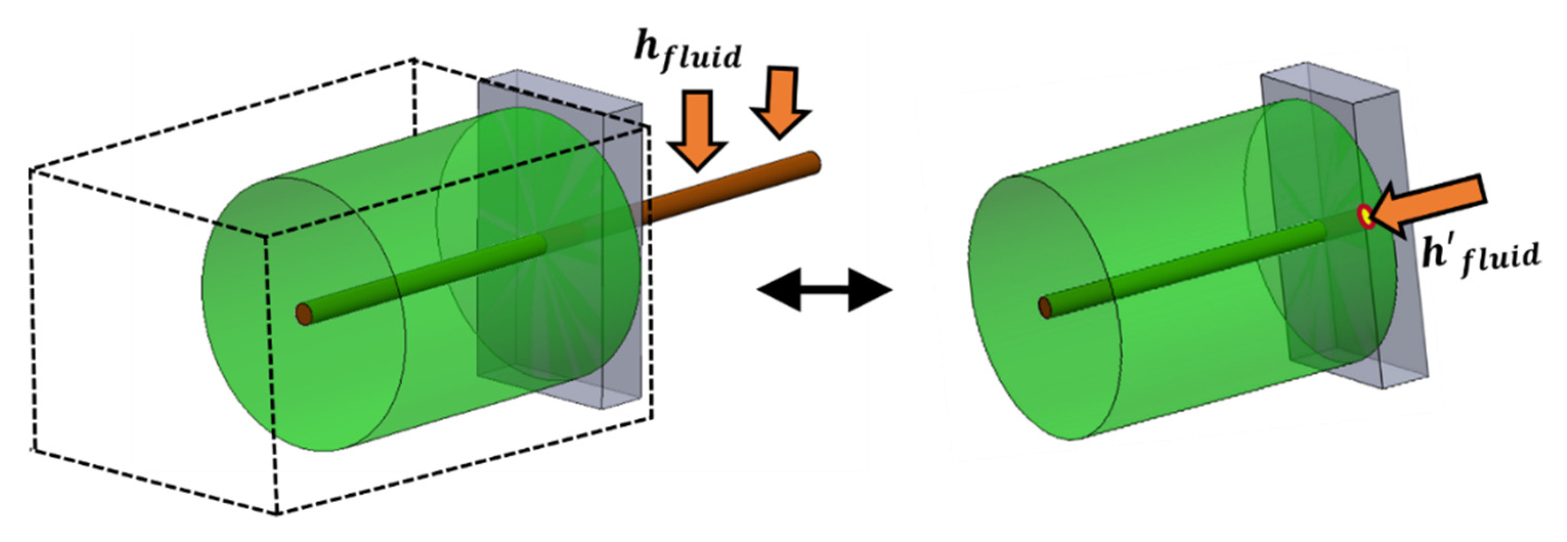
Calculation of Fluid Convective Resistance,
Calculation of Wire Conductive Resistance,
Calculation of PCM Conductive Resistance,
3.3.2. Latent Energy Stored in a Single Row,
3.3.3. Latent Energy Stored in Entire TES,
3.3.4. Time-Integrated Latent Energy Stored in Entire TES,
3.4. Non-Dimensionalized Form of Governing Equations
3.5. Model Input and Outputs
4. 2D CFD Cartesian Model ( Plane)
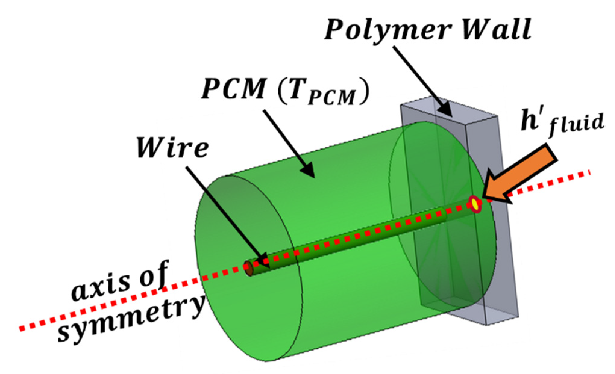
5. 2D CFD Axisymmetric Model ( Plane)
6. Results and Discussion
6.1. Test-Case Setup
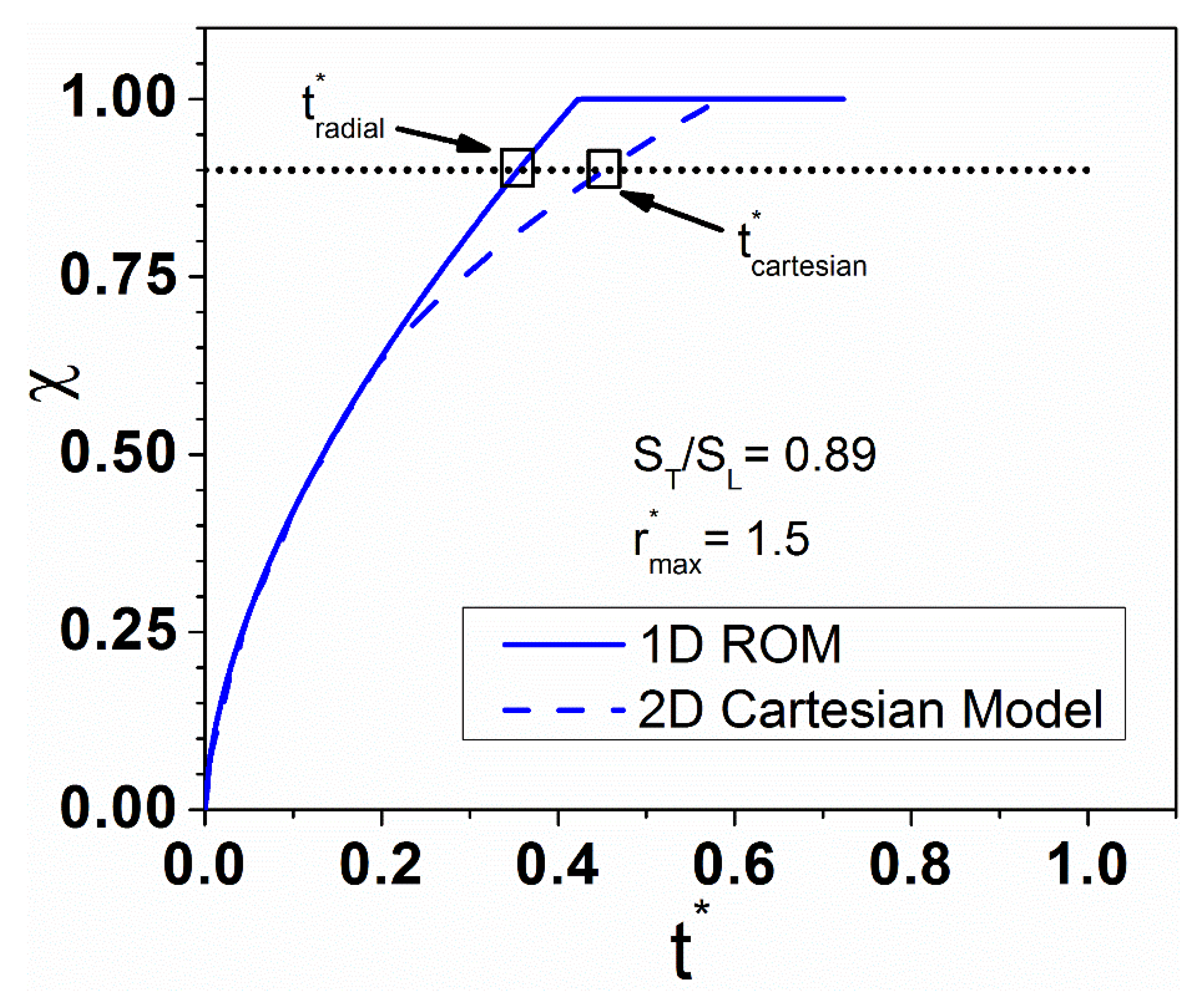
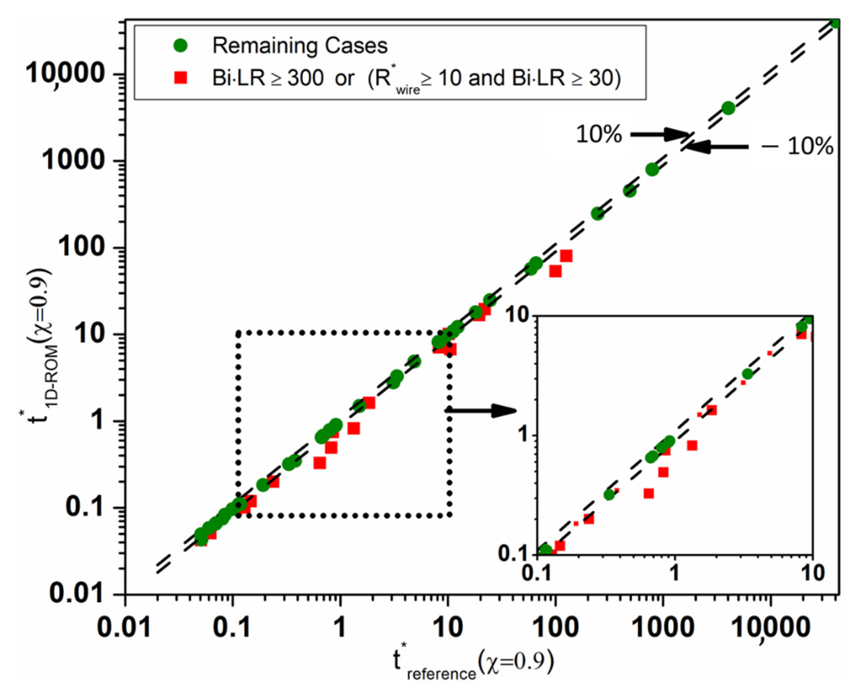
6.2. Validation with the Widely-Used 2D CFD Axisymmetric Model
6.2.1. Parametric Case Study
Effect of
Effect of
Effect of
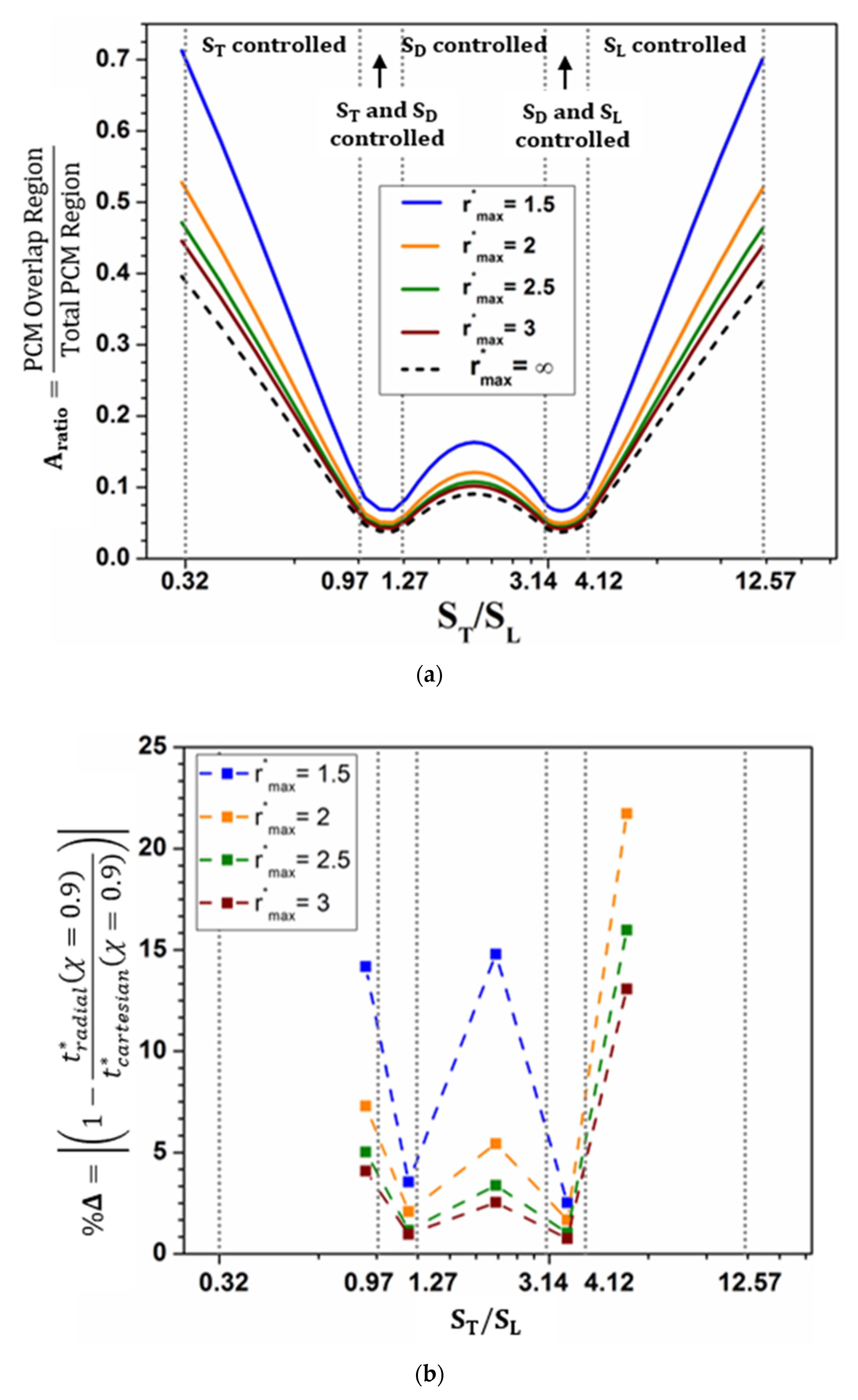
6.2.2. Multi-Dimensional Parametric Study
7. Conclusions
Author Contributions
Funding
Institutional Review Board Statement
Informed Consent Statement
Data Availability Statement
Acknowledgments
Conflicts of Interest
Nomenclature
| A | area, m2 |
| b | fin parameter |
| Bi | Biot number |
| specific heat capacity, W/kg⋅K | |
| D | diameter of wire, m |
| latent energy stored in a single-wire PCM matrix, J | |
| total latent energy stored in a single row of wire-PCM matrices, J | |
| TES latent energy at a known time, J | |
| time-integrated total TES latent energy, J | |
| Fo | Fourier number |
| fluid heat transfer coefficient acting circumferentially on wire exposed to fluid side, W/m2⋅K | |
| fluid heat transfer coefficient acting on cross-sectional area of wire exposed to PCM side on 3D plane, | |
| fluid heat transfer coefficient acting on cross-sectional area of wire exposed to PCM side on 2D plane, | |
| H | latent heat of fusion, J/kg |
| k | thermal conductivity, W/m⋅K |
| L | length, m |
| corrective fin length, m | |
| m | mass, kg |
| mass of transitioned PCM, kg | |
| maximum mass of non-transitioned PCM, kg | |
| fluid mass flow rate, kg/s | |
| n | number of channels |
| N | number of wires |
| pressure drop of fluid, Pa | |
| nominal heat transfer rate, W | |
| maximum heat transfer rate, W | |
| equivalent heat transfer rate, W | |
| wire radius, m | |
| r | melt-front radius of PCM, m |
| R | resistance, K/W |
| steady state cylindrical resistance for radial conduction, | |
| S | center-to-center spacing between neighboring wires, m |
| Ste | Stefan number |
| specified time, s | |
| t | time, s |
| time-step, s | |
| wall thickness, m | |
| T | temperature, |
| W | width of channels, m |
| Greek Symbols | |
| wire sector angle in direction of or , radians | |
| wire sector angle in direction of , radians | |
| liquid fraction | |
| difference | |
| fin efficiency | |
| density, kg/m3 | |
| dimensionless time constant | |
| dimensionless temperature difference ratio | |
| Subscripts | |
| 0 | nominal |
| c | cross-sectional area |
| cartesian | Cartesian coordinate plane |
| cond | conductive |
| cylinder | cylindrical surface |
| D | diagonal |
| fluid | related to fluid side |
| in | inlet |
| L | longitudinal direction to flow |
| max | maximum |
| out | outlet |
| overlap | related to PCM overlap |
| PCM | related to phase change material side |
| radial | radial coordinate plane |
| ratio | dimensionless parameter |
| T | transverse direction to flow |
| wire | related to metal wire |
| Superscripts | |
| * | dimensionless ratio |
| surf | surface |
| Abbreviations | |
| CFD | computational fluid dynamics |
| Diff | difference |
| HX | heat exchanger |
| LHS | left hand side |
| LR | length ratio |
| PCM | phase change material |
| RHS | right hand side |
| ROM | reduced-order model |
| TES | thermal energy storage |
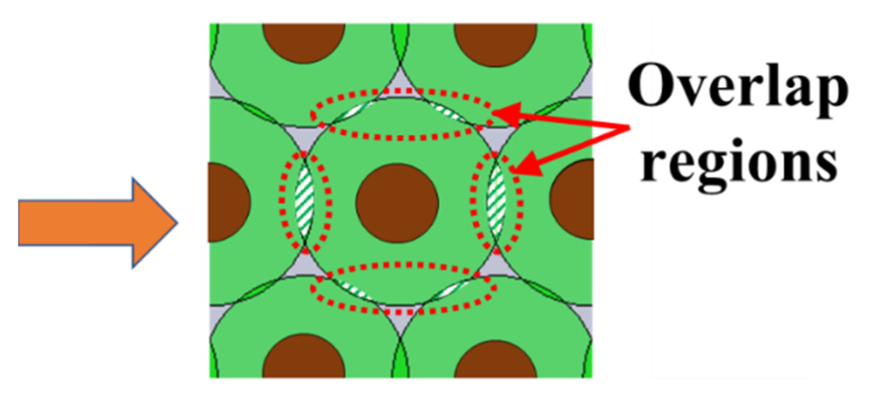
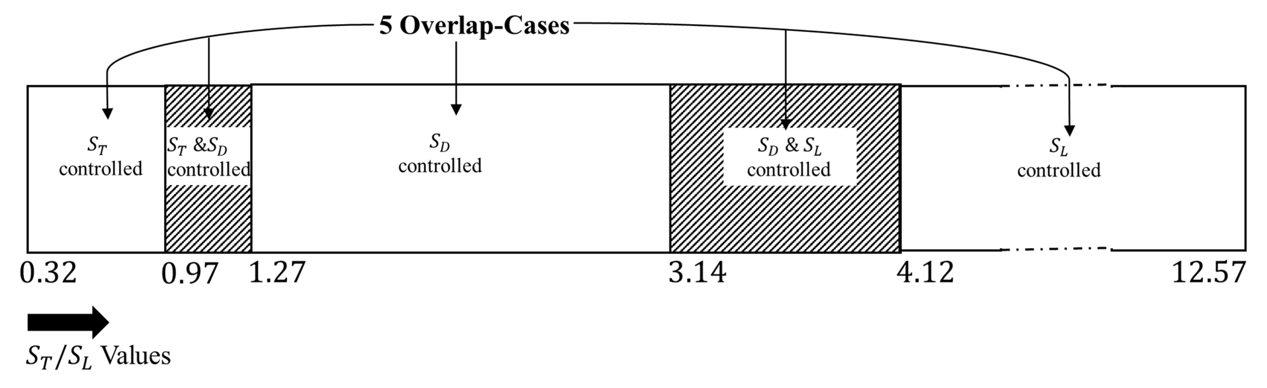
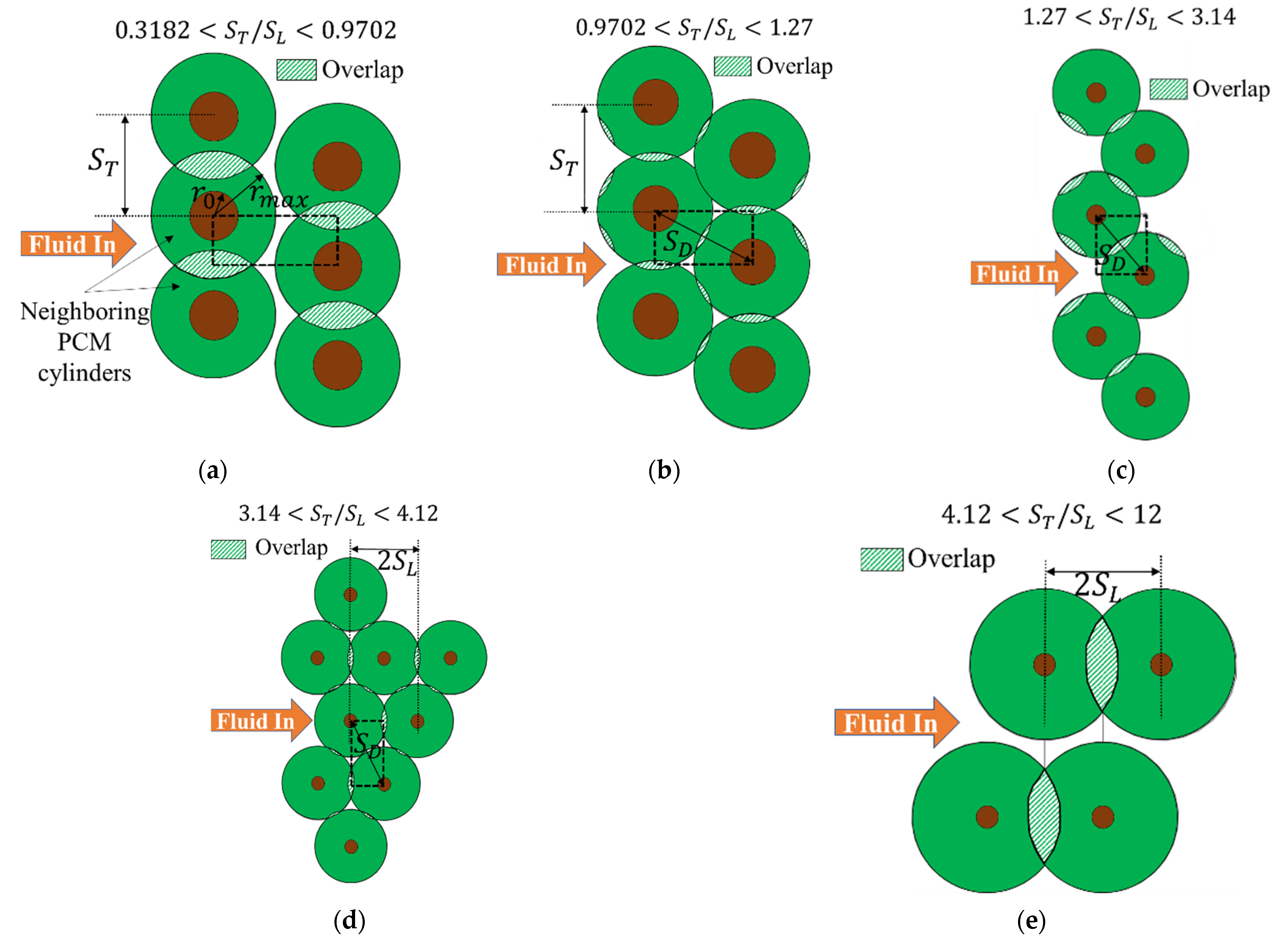
Appendix A. Range of Overlaps
- Overlap in direction of orcontrolled
- Overlap in direction oforcontrolled
- Overlap in direction oforcontrolled
Appendix B. Geometric Behavior of Overlap Regions
Appendix C. Non-Dimensionalization of Main Governing Equation of 1D ROM
Appendix D. Limiting Conditions:
References
- Pasupathy, A.; Athanasius, L.; Velraj, R.; Seeniraj, R.V. Experimental investigation and numerical simulation analysis on the thermal performance of a building roof incorporating phase change material (PCM) for thermal management. Appl. Therm. Eng. 2008, 28, 556–565. [Google Scholar] [CrossRef]
- Qu, S.; Ma, F.; Ji, R.; Wang, D.; Yang, L. System design and energy performance of a solar heat pump heating system with dual-tank latent heat storage. Energy Build. 2015, 105, 294–301. [Google Scholar] [CrossRef]
- Gholamibozanjani, G.; Farid, M. Peak load shifting using a price-based control in PCM-enhanced buildings. Sol. Energy 2020, 211, 661–673. [Google Scholar] [CrossRef]
- Shao, W.; Ran, L.; Zeng, Z.; Wu, R.; Mawby, P.; Huaping, J.; Kastha, D.; Bajpai, P. Power modules for pulsed power applications using phase change material. In Proceedings of the 2018 Second International Symposium on 3D Power Electronics Integration and Manufacturing (3D-PEIM), College Park, MD, USA, 25–27 June 2018. [Google Scholar] [CrossRef]
- Lafdi, K.; Mesalhy, O.; Elgafy, A. Graphite foams infiltrated with phase change materials as alternative materials for space and terrestrial thermal energy storage applications. Carbon 2008, 46, 159–168. [Google Scholar] [CrossRef]
- Choi, D.H.; Lee, J.; Hong, H.; Kang, Y.T. Thermal conductivity and heat transfer performance enhancement of phase change materials (PCM) containing carbon additives for heat storage application. Int. J. Refrig. 2014, 42, 112–120. [Google Scholar] [CrossRef]
- Singh, R.; Sadeghi, S.; Shabani, B. Thermal conductivity enhancement of phase change materials for low-temperature thermal energy storage applications. Energies 2019, 12, 75. [Google Scholar] [CrossRef] [Green Version]
- Milián, Y.E.; Gutiérrez, A.; Grágeda, M.; Ushak, S. A review on encapsulation techniques for inorganic phase change materials and the influence on their thermophysical properties. Renew. Sustain. Energy Rev. 2017, 73, 983–999. [Google Scholar] [CrossRef]
- Höhlein, S.; König-Haagen, A.; Brüggemann, D. Macro-Encapsulation of Inorganic Phase-Change Materials (PCM) in Metal Capsules. Materials 2018, 11, 1752. [Google Scholar] [CrossRef] [Green Version]
- Kailkhura, G.; Mandel, R.K.; Shooshtari, A.H.; Ohadi, M.M. Experimental study of a set of integrated cross-media heat exchangers (iCMHXs) for liquid cooling applications in desktop computers. In InterPACK 2020; Cambridge University Press: Cambridge, UK, 2020; pp. 1–58. [Google Scholar] [CrossRef]
- Kailkhura, G.; Mandel, R.K.; Shooshtari, A.H.; Ohadi, M.M. Numerical Investigation of an Integrated Cross-Media Heat Exchanger (iCMHX) for Gas-to-Liquid Cooling Applications. In Proceedings of the IEEE Intersociety Conference on Thermal and Thermomechanical Phenomena in Electronic Systems (iTherm), Orlando, FL, USA, 21–23 July 2020. [Google Scholar]
- Arie, M.; Hymas, D.; Singer, F.; Shooshtari, A.; Ohadi, M. Performance characterization of a novel cross-media composite heat exchanger for air-to-liquid applications. In Proceedings of the 18th IEEE Intersociety Conference on Thermal and Thermomechanical Phenomena in Electronic Systems (ITherm), Las Vegas, NV, USA, 28–31 May 2019; pp. 933–940. [Google Scholar] [CrossRef]
- Arie, M.A.; Hymas, D.M.; Singer, F.; Shooshtari, A.H.; Ohadi, M. An additively manufactured novel polymer composite heat exchanger for dry cooling applications. Int. J. Heat Mass Transf. 2020, 147, 118889. [Google Scholar] [CrossRef]
- Kailkhura, G.; Mandel, R.K.; Shooshtari, A.; Ohadi, M. Numerical and Experimental Study of a Novel Additively Manufactured Metal-Polymer Composite Heat-Exchanger for Liquid Cooling Electronics. Energies 2022, 15, 598. [Google Scholar] [CrossRef]
- Lane, G.A. Background and scientific principles. In Solar Heat Storage: Latent Heat Material, 1st ed.; Lane, G.A., Ed.; CRC Press: Boca Raton, FL, USA, 2018. [Google Scholar] [CrossRef]
- Stefan, J. Ueber die Theorie der Eisbildung, insbesondere über die Eisbildung im Polarmeere. Ann. Phys. 1891, 278, 269–286. [Google Scholar] [CrossRef] [Green Version]
- Jiji, L.M. Heat Conduction, 3rd ed.; Springer: Berlin/Heidelberg, Germany, 2009; pp. 1–418. [Google Scholar] [CrossRef]
- Lane, G.A. Solar Heat Storage: Latent Heat Material: Volume II: Technology; CRC Press: Boca Raton, FL, USA, 2018; pp. 1–235. [Google Scholar] [CrossRef]
- Al-Saadi, S.N.; Zhai, Z. Modeling phase change materials embedded in building enclosure: A review. Renew. Sustain. Energy Rev. 2013, 21, 659–673. [Google Scholar] [CrossRef]
- Ehms, J.H.N.; De Césaro Oliveski, R.; Rocha, L.A.O.; Biserni, C.; Garai, M. Fixed Grid Numerical Models for Solidification and Melting of Phase Change Materials (PCMs). Appl. Sci. 2019, 9, 4334. [Google Scholar] [CrossRef] [Green Version]
- Dutil, Y.; Rousse, D.R.; Salah NBen Lassue, S.; Zalewski, L. A review on phase-change materials: Mathematical modeling and simulations. Renew. Sustain. Energy Rev. 2011, 5, 112–130. [Google Scholar] [CrossRef]
- Trp, A. An experimental and numerical investigation of heat transfer during technical grade paraffin melting and solidification in a shell-and-tube latent thermal energy storage unit. Sol. Energy 2005, 79, 648–660. [Google Scholar] [CrossRef]
- Kozak, Y.; Ziskind, G. Novel enthalpy method for modeling of PCM melting accompanied by sinking of the solid phase. Int. J. Heat Mass Transf. 2017, 112, 568–586. [Google Scholar] [CrossRef]
- Hu, Y.; Guo, R.; Heiselberg, P.K.; Johra, H. Modeling PCM Phase Change Temperature and Hysteresis in Ventilation Cooling and Heating Applications. Energies 2020, 13, 6455. [Google Scholar] [CrossRef]
- Pan, C.; Hoenig, S.; Chen, C.H.; Neti, S.; Romero, C.; Vermaak, N. Efficient modeling of phase change material solidification with multidimensional fins. Int. J. Heat Mass Transf. 2017, 115, 897–909. [Google Scholar] [CrossRef]
- Heim, D.; Heim, D. Two solution methods of heat transfer with phase change within whole building dynamic simulation. In Proceedings of the 9th International IBPSA Conference, Roma, Italy, 2–4 September 2019; Available online: http://citeseerx.ist.psu.edu/viewdoc/summary?doi=10.1.1.577.5744 (accessed on 17 January 2022).
- Khattari, Y.; El Rhafiki, T.; Choab, N.; Kousksou, T.; Alaphilippe, M.; Zeraouli, Y. Apparent heat capacity method to investigate heat transfer in a composite phase change material. J. Energy Storage. 2020, 28, 101239. [Google Scholar] [CrossRef]
- Gong, Z.X.; Mujumdar, A.S. Finite-element analysis of cyclic heat transfer in a shell-and-tube latent heat energy storage exchanger. Appl. Therm. Eng. 1997, 17, 583–591. [Google Scholar] [CrossRef]
- Ismail, K.A.R.; Alves, C.L.F.; Modesto, M.S. Numerical and experimental study on the solidification of PCM around a vertical axially finned isothermal cylinder. Appl. Therm. Eng. 2001, 21, 53–77. [Google Scholar] [CrossRef]
- Zauner, C.; Hengstberger, F.; Etzel, M.; Lager, D.; Hofmann, R.; Walter, H. Experimental characterization and simulation of a fin-tube latent heat storage using high density polyethylene as PCM. Appl. Energy 2016, 179, 237–246. [Google Scholar] [CrossRef]
- Huang, K.; Feng, G.; Zhang, J. Experimental and numerical study on phase change material floor in solar water heating system with a new design. Sol. Energy 2014, 105, 126–138. [Google Scholar] [CrossRef]
- El-Dessouky, H.; Al-Juwayhel, F. Effectiveness of a thermal energy storage system using phase-change materials. Energy Convers. Manag. 1997, 38, 601–617. [Google Scholar] [CrossRef]
- Bansal, N.K.; Buddhi, D. An analytical study of a latent heat storage system in a cylinder. Energy Convers. Manag. 1992, 33, 235–242. [Google Scholar] [CrossRef]
- Jian-you, L. Numerical and experimental investigation for heat transfer in triplex concentric tube with phase change material for thermal energy storage. Sol. Energy 2008, 82, 977–985. [Google Scholar] [CrossRef]
- Ayyagari, V.; Kailkhura, G.; Mandel, R.K.; Shooshtari, A.; Ohadi, M. Performance Characterization of a Novel Low-Cost Additively Manufactured PCM-to-Air Polymer Composite Thermal Energy Storage for Cooling Equipment Peak Load Shifting. In Proceedings of the 21st IEEE Intersociety Conference on Thermal and Thermomechanical Phenomena in Electronic Systems (ITherm), San Diego, CA, USA, 31 May–3 June 2022. [Google Scholar]
- Hymas, D.; Dessiatoun, S.; Ohadi, M.M. Metal/Polymer Composite Additive Manufacturing (mfc-am) and Composite Structures Formed by mfc-am. U.S. Patent and Trademark Office 62,405,085, 12 April 2018. [Google Scholar]
- Mehling, H.; Luisa, F. Cabeza. Heat and cold storage with PCM. J. Vis. Lang. Computing. 2000, 11, 287–301. [Google Scholar]
- Bergman, T.L.; Lavine, A.S.; Incropera, F.P.; DeWitt, D.P. Fundamentals of Heat and Mass Transfer; John Wiley & Sons: Hoboken, NJ, USA, 2011. [Google Scholar]
- ANSYS FLUENT 12.0 Theory Guide—17.4 Energy Equation. Available online: https://www.afs.enea.it/project/neptunius/docs/fluent/html/th/node353.htm (accessed on 10 November 2021).


| Non-Dimensional Groups | Mathematical Definition | Physical Meaning |
|---|---|---|
| Time-constant | ||
| Proportional to the ratio of axial conductive resistance of the wire embedded in PCM to fluid-side resistance | ||
| Proportional to the ratio of axial conductive resistance of the wire embedded in PCM to maximum radial resistance of PCM |
| 0.2 | 6 | 400 | 1.2 | 3 | 3.68 | 37.5 | 1.943 |
| ) | %Diff | ||
| 0.02 | 300 | 0.878 | - |
| 0.01 | 600 | 0.887 | 1% |
| 0.005 | 1200 | 0.89 | 0.38% |
Publisher’s Note: MDPI stays neutral with regard to jurisdictional claims in published maps and institutional affiliations. |
© 2022 by the authors. Licensee MDPI, Basel, Switzerland. This article is an open access article distributed under the terms and conditions of the Creative Commons Attribution (CC BY) license (https://creativecommons.org/licenses/by/4.0/).
Share and Cite
Kailkhura, G.; Mandel, R.K.; Shooshtari, A.; Ohadi, M. A 1D Reduced-Order Model (ROM) for a Novel Latent Thermal Energy Storage System. Energies 2022, 15, 5124. https://doi.org/10.3390/en15145124
Kailkhura G, Mandel RK, Shooshtari A, Ohadi M. A 1D Reduced-Order Model (ROM) for a Novel Latent Thermal Energy Storage System. Energies. 2022; 15(14):5124. https://doi.org/10.3390/en15145124
Chicago/Turabian StyleKailkhura, Gargi, Raphael Kahat Mandel, Amir Shooshtari, and Michael Ohadi. 2022. "A 1D Reduced-Order Model (ROM) for a Novel Latent Thermal Energy Storage System" Energies 15, no. 14: 5124. https://doi.org/10.3390/en15145124
APA StyleKailkhura, G., Mandel, R. K., Shooshtari, A., & Ohadi, M. (2022). A 1D Reduced-Order Model (ROM) for a Novel Latent Thermal Energy Storage System. Energies, 15(14), 5124. https://doi.org/10.3390/en15145124