Multi-Chamber Actuator Mode Selection through Reinforcement Learning–Simulations and Experiments

Abstract

This paper presents the development and implementation of a reinforcement learning agent as the mode selector for a multi-chamber actuator in a load-sensing architecture. The agent selects the mode of the actuator to minimise system energy losses. The agent was trained in a simulated environment and afterwards deployed to the real system. Simulation results indicated the capability of the agent to reduce energy consumption, while maintaining the actuation performance. Experimental results showed the capability of the agent to learn via simulation and to control the real system.

1. Introduction

In a multiple hydraulic actuator system, the load on each actuator results in different pressure levels. If the actuators are controlled by a load-sensing architecture with pressure-compensation valves and a single pump, the supply pressure is controlled according to the highest required pressure. This causes a mismatch between the pressures in the actuators and the supply that is compensated for by the throttling on the pressure-compensation valves. These resistive control losses are one of the major sources of energy losses in such hydraulic systems [1,2].

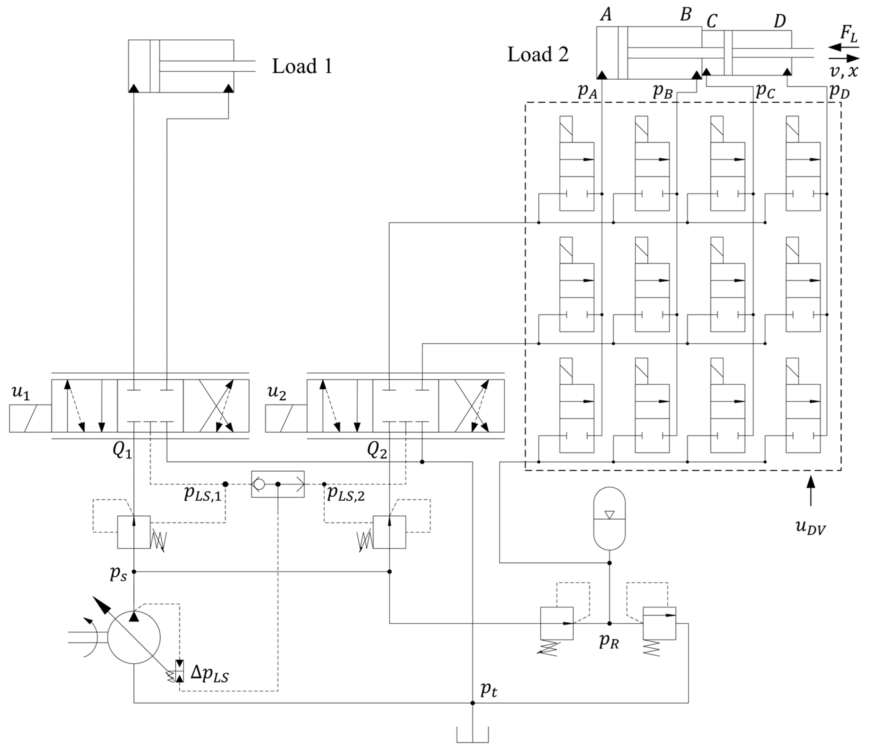
One way of reducing such losses is to use a multi-chamber actuator in one of the loads. A hydraulic diagram of a pressure-compensated valve-controlled load-sensing architecture, where Load 2 is driven by a multi-chamber actuator, is shown in Figure 1.

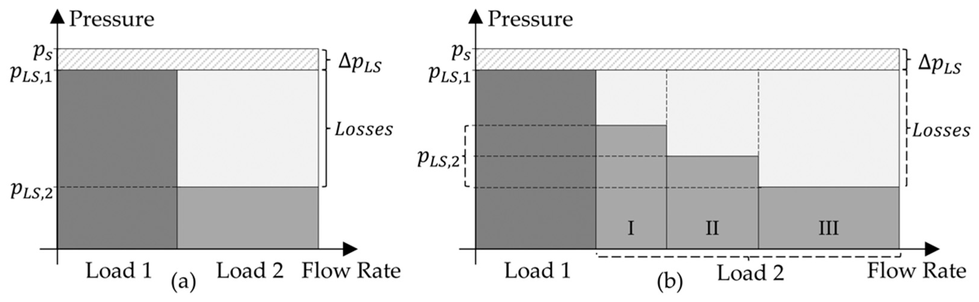
The set of on/off valves between the proportional valve and the actuator allows for the combinations of different chambers that define the possible actuator modes to be used. The capability to select different actuator modes allows the modulation of the resultant pressure from the load to make $p_{LS,2}$ similar to $p_{LS,1}$. This is shown in the illustrative flow-pressure diagrams in Figure 2.

The possibility to modulate the pressure, Figure 2b, enables the reduction in resistive control losses. A conventional actuator, Figure 2a, cannot perform this modulation and, thus, results in higher resistive control losses. A deeper discussion on this system architecture is provided in [3].

This architecture has another degree of freedom to be controlled, which is the mode selection. The mode that minimises the losses is a function of the speed and forces of all the actuators, but because these vary along with the system operation, this is not a trivial problem to solve.

Multi-chamber actuators usually belong to architectures where the selection of modes is responsible for the control end goal, such as speed or position. The speed or position error is translated to a reference force that the multi-chamber actuator must exert. In [4], this force reference is compared to the available forces for each mode, and the mode that results in the smallest force error is applied to the system. In [5], a mode selection based on the minimisation of the force error is implemented, as in [4]; however, there is no mention of avoiding frequent switching. In [6], the same mode-selection strategy as in [4] is compared to one that penalizes high-amplitude pressure changes between different modes. In [7], the authors describe the operation of a controller that selects the mode that minimises the energy consumption, while still being able to drive the current load. In [8], the mode selection is also based on a predefined range of force capacity for each mode. The implemented mode is the one that can exert the requested force, and the difference in force is controlled by the proportional pressure control in one of the chambers.

Model predictive control (MPC) is studied in [9] to solve the problems related to force spikes when in mode switching. The mode selection is still performed based on minimising the force difference between the reference and the available modes and on minimising the energy losses associated with switching. The force difference is handled by means of throttle control, to adjust the pressure in each chamber to the calculated pressure reference. MPC is focused on minimising the force transients when switching. A similar study also using MPC is presented in [10], where the results also indicate an advantage of MPC over simpler mode-selection strategies, as presented in [4], for example.

Although not used for a multi-chamber actuator, the selection of modes in [2] is performed based on the calculation of the capacity of each mode to overcome the current force over the actuator, while, apparently, minimising the pump pressure and flow rate.

The authors in [11] describe a state machine to handle the mode selection based on, for example, the load pressure and pressure levels defined for each mode. The authors emphasise possible instability and non-smooth operation of the actuator during mode switching and suggest that these problems could be minimised by acting on the proportional valve control, which to some extent follows the ideas presented in [8,9]. In [12], the mode selection of the independent metering valve system is also performed based on the current load force and the force capability of each mode.

The control problem here is not the same as the ones studied by the works presented above. Here, the mode selection acts as an enabler for the control end goal, which is still performed by the proportional valve. Therefore, the control goal for the multi-chamber actuator is to select a mode that enables the requested motion to be completed, while minimising the resistive control losses. From another point of view, the mode selector can be interpreted as performing energy management because the goal of using the multi-chamber actuator is to reduce energy losses. Instead of designing a controller for the mode selection based on the analytical equations of the energy losses in the system, in this work a controller for the mode selection based on RL was studied.

Reinforcement learning (RL), with neural networks as the actor and critic function approximators, has proven to be a powerful and successful control-development methodology for complex problems, such as playing Atari [13]. The main advantages are automatic learning by interacting with the environment and finding optimised control solutions that are inherently difficult to be solved analytically. Additionally, machine learning algorithms also perform well in scenarios that they are not exactly trained for, which is likely to occur in the operation of mobile machines, due to their vast field of application.

In the control of mobile working machines, Ref. [14] presents an approach based on RL, with the Q-learning algorithm for the control of hybrid system power to minimise fuel consumption. What the authors also show is the possibility of first training the controller with simulation models of the system and then applying the controller to the real system. An RL-based energy-management strategy is proposed in [15] for hybrid construction machines. The authors use a combination of Dyna learning and Q-learning, but the study is limited to simulation results.

Other applications of RL for mobile machines include: Ref. [16], where it is used, based on cameras, lidar, and motion and force sensors, to perform bucket loading of fragmented rock with a multi-objective target, including maximisation of the bucket loading; Ref. [17], where it is trained for the motion control of a forestry crane while minimising energy consumption; and Ref. [18], where it is used for the trajectory tracking control of an excavator arm, with the controller generating the valve-control signals directly.

It is observed in these papers that the development of RL controllers usually starts with a pre-training of the agent in a simulation environment. Advantages of this approach are: it avoids undesirable real-world consequences; it reduces costs associated with obtaining real experience; and the simulations typically run faster than real time [19]. The reviewed papers also show the controller’s capacity to find and implement solutions for complex tasks.

This paper demonstrates, through simulation and experimental results, the training and implementation of a RL-based controller for the mode selection of a multi-chamber hydraulic actuator. The actuator is part of a multi-actuator load-sensing architecture driven by a single pump. The selection of different modes allows for the reduction in resistive losses in the control valves, due to a better match of pressures between actuators. A Deep Q-Learning (DQN) agent was created and trained to learn how to select the modes to minimise the system energy losses.

Paper Contribution and Objectives

Research on the topic of this paper has been presented in previous publications by our group. In [3], the system architecture is described along with the potential efficiency improvements. The first implementation of the RL-based approach to control this system was studied and presented in [20]. The present work builds on those previous publications, where the main difference from [20] is the use of a load-sensing pump instead a constant pressure supply, which makes the learning task significantly harder and closer to a real, mobile system application.

The objective and, consequently, the contribution of this paper are to show experimental results demonstrating that RL can also be used to control complex hydraulic systems. In this case, it is about the selection of modes of multi-chamber actuators aiming to reduce resistive control losses. In particular, it is shown that RL finds an optimised control solution with reduced need for manually designing the controller. However, the study is limited to training the agent in simulation and not on continuing the learning after being deployed to the real system.

2. Available Modes, Model Description, and Control Structure

The multi-chamber actuator used in this study has four chambers and is connected to three supply lines (A/B/R). This gives a total of 87 possible modes. However, most modes are ruled out due to the reasons presented in [3]. The modes used in this study are given in

Table 1. Available modes and connected chambers.

Mode	A	B	R	Force [kN]
1	-	-	-	-
2	AC	BD	-	77
3	ABC	D	-	70
4	A	BD	C	55
5	AB	D	C	48
6	C	BD	A	12

. Mode 1 is the only mode that is not an agent’s decision, because it is implemented as a rule to ensure safe operation. The steady state force displayed in Table 1 is calculated considering a pressure of 100 bar on port A and 15 bar on ports B and R. This is done to show which modes can exert higher force.

The model of the physical system was developed in the multi-domain system simulation tool HOPSAN [21] and describes the motion of the boom arm as a function of the motion of the actuators. It also models the dynamic behaviour of the pressures, flow rates, internal leakage, and closing and opening of the valves. The model was validated against experimental results, with a detailed description presented in [20].

The controller and training algorithm for the DQN agent were implemented in MATLAB/Simulink [21]. During the training in simulation, the agent learns by interacting with the system. After training, the agent controls the real system.

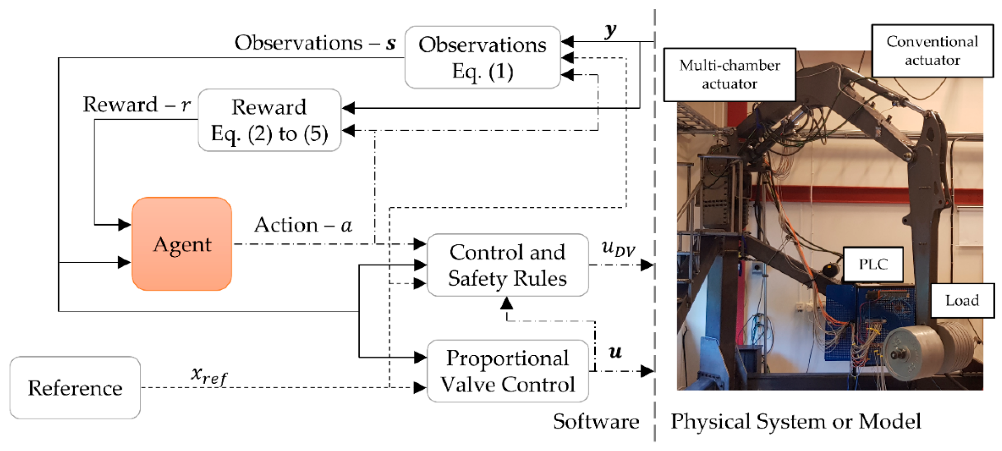
The actual controller of the system is not only composed of the trained agent selecting the optimal mode, it also contains other control and safety rules. An overview of the controller structure is shown in Figure 3. The reward branch of the agent is only used during the training phase.

In Figure 3, it is also seen how the interaction of the agent with the environment takes place during the learning phase and then in the controlling phase. Paraphrasing [13] for the present control problem: The agent interacts with the environment in a sequence of actions, observations, and rewards. At each agent time step $\left(t\right)$, the agent observes the observations $s\left(t\right)$, selects an action $a\left(t\right)$ from the set of modes (Table 1), and applies it to the environment. It observes the new observations $s\left(t+1\right)$ and the reward $r\left(t\right)$. It tries to maximise the reward.

From the RL perspective, everything that is not the agent is considered as the environment it is interacting with. It is important to make the environment in the simulation as close to the real environment as possible. For the control of hydraulic systems in mobile applications, along with having a sufficiently accurate model of the physical system, there is the need to include additional safety rules. Therefore, the environment is the combination of the system model and the additional rules. The added control and safety rules for this system are:

• Apply mode 1 if $\left|u_2\right|<0.002 \mathrm{m}$;
• Limit the available modes according to position and external load;
• Compensate $u_2$ due to the difference in areas in each mode; and
• Use mode 4 for the lowering motion ($u_2$ < $-$0.002 m).

The first rule is used because the valve has an overlap of 2 mm, so the on/off valves can be closed. The second rule prevents the agent from choosing a mode that cannot drive the load with the available maximum pump pressure, otherwise the load could fall. For the same operator control input signal to the proportional valve, the third rule ensures approximately the same actuator speed for the different modes, see [3,20] for details.

The fourth rule is implemented because the return motion, due to the much larger area of the actuator connected to the return than the supply, results in excessive throttling on the meter-out edge of the valve. This causes the pump to operate at maximum pressure due to a perceived high load, which causes the pressure-compensation valves to operate fully open and, thus, the compensation losses are close to zero. Thus, the selection of modes, based on minimising the compensation losses, does not work for the returning motion. Therefore, due to this design constraint, the return motion is not an agent’s decision.

While the RL agent is responsible for the mode selection, another P controller ’mimics’ the machine operator controlling the proportional valves. The P controller is implemented inside the proportional valves control block in Figure 3.

3. Learning Setup for the Agent

The application has a continuous observation space (pressures, speed, etc.) and a discrete action space (modes to be selected). A DQN agent [13,22] is suitable for this type of observation and action space, and it mainly consists of a neural network calculating the value for taking a certain action given the current observations. The value is an estimation of the sum of the reward that the agent can collect over a future time horizon, by following a certain sequence of control actions. In this case, the network at each agent’s time step predicts the value of taking each action. A greedy function selects and implements in the system the action that has the highest estimated value, which is, in other words, the action that would lead to the best performance, according to the reward function. This agent is, thus, a non-linear map between the system states (observations of pressures, speed, position, …) and the optimised control action (modes). The reader is referred to [13,22] for a description of the type of agent and training algorithm.

Each agent action corresponds to one mode (Table 1). Inside the ‘Control and Safety Rules’ block in Figure 3, a lookup table maps the action to the corresponding vector $u_{DV}$ of the open/closed digital valves that implements the mode in the system.

The structure and parameters of the network are presented in

Table 2. Structure of the agent network.

Layer	Size
Feature inputs (observations)	9 input features
Fully connected with Rectified Linear Unit activation function	70 neurons
Fully connected with Rectified Linear Unit activation function	35 neurons
Fully connected output (actions)	5 neurons

. No sensitivity analysis was performed to evaluate the size of the network on the performance of the task. However, the size of the network was chosen to be small.

The observations $\mathit{s}$ used as input features are

$$\mathit{s}\left(t\right)=\left[a,u_2,p_A,p_B,p_C,p_s,p_{LS,1},v,x\right],$$

(1)

where $a$ is the previous action, $u_2$ is the proportional valve control signal, $p_{A-B-C}$ are the chambers’ pressures, $p_s$ is the supply pressure, $p_{LS,1}$ is the load-sensing pressure for the conventional actuator, $v$ is the actuator speed, and $x$ is the position.

The reward function $r$ to be maximised is composed of three terms,

$$r=K_1{r}_{Velocity}+K_2{r}_{Power}+K_3{r}_{Switch},$$

(2)

$$r_{Velocity}=-1 if \left|v\right|<0.001 \mathrm{m}/\mathrm{s},$$

(3)

$$r_{Power}=-\left(\left|Q_2\left(p_s-p_{LS,2}\right)\right|+\left| Q_1\left(p_s-p_{LS,1}\right)\right|\right)/P_{Norm},$$

(4)

$$r_{Switch}=\{\begin{array}{cc}{r}_{Switch} & if a_{t+1}=a_t\\ r_{Switch}-1& if a_{t+1}\ne a_t\end{array}.$$

(5)

The velocity term ($r_{Velocity}$) penalizes the agent if a motion is requested ($\left|u_2\right|>0.002$), and the multi-chamber actuator does not move with a minimum velocity. This encourages the agent to learn to meet a minimum control-performance requirement. The power loss term ($r_{Power}$) is a penalty based on the hydraulic system control losses, to encourage the agent to find a mode that results in smaller energy losses due to pressure compensation. The switch term ($r_{Switch}$) penalizes the agent for frequent mode switching.

Table 3. Agent and task parameters.

Parameter	Value
Initial exploration factor	$0.99$
Minimum exploration factor	0.15
Exploration factor decay	$7.5\times {10}^{-6}$
Target smooth factor	$2.0\times {10}^{-3}$
Learning rate	$7.5\times {10}^{-4}$
Mini-batch size	$128$
Look ahead steps	$4$
Experience buffer length	$4.0\times {10}^4$
Agents sample time [s]	$0.80$
Discount factor	$0.99$
Gradient decay factor	$0.9$0
Maximum number of episodes	$1.8\times {10}^4$
Load Cases and Task	Value
Initial position [m]	$0.10+0.02R$
Final position [m]	$0.40+0.05R$
External load [kg]	$\left[40 80 120 160 200 240\right]$
$\mathrm{Load}1\mathrm{load}\mathrm{sensing}\mathrm{pressure}{p}_{LS,1}$ [bar]	$\left[60 100\right] \pm 3R$
$\mathrm{Load}1\mathrm{flow}\mathrm{rate}{Q}_1$ [lpm]	$10$

presents the parameters and load cases used during training. To increase the agent’s robustness, noise is added to the measurements used as observations in the simulations. $R$ is a uniformly distributed random variable with a maximum amplitude of 1.

In a real system, the load pressure from the conventional actuator ($p_{LS,1}$) varies according to the load. However, a simplification is made by setting it to constant values to allow for easier interpretation of the results both in the simulation and in the experiments. In the experiments, this signal is emulated with an additional hydraulic circuit. This means that the agent is exposed to 12 different scenarios of external load and pressure on the conventional actuator, and the task is to lift the load from an initial position to a final position while maximising the reward function.

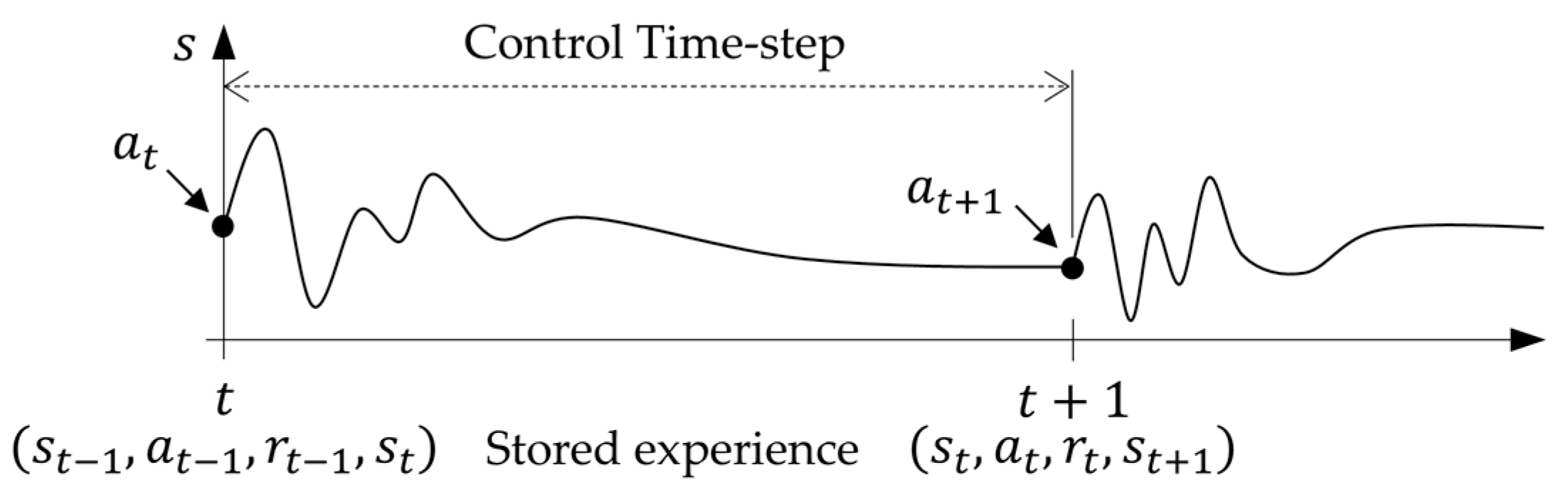
Dynamic systems have oscillations, and these must be taken into consideration when setting the agent-control time step, defining the reward function, and considering what type of information is stored as experience. This is represented in Figure 4, by showing a dynamic response of the system state ($s$) due to an action $a_t$.

If the time step is too small, the stored experience will contain dynamic effects rather than steady-state conditions. This might affect the agent’s ability to learn because the reward function could give misinformation. However, the reward from the action at $t$ is only observed at $t+1$ because it is usually a function of the final state and the transition between the states. Therefore, the size of the control time step can be adjusted to avoid these effects. For the current system, the mode selection does not need to occur frequently to avoid unnecessary switching. Thus, the agent time step is set to avoid these oscillations.

4. Results

The agent was trained to lift a load from a certain initial position to a final position, with 12 load cases that including 2 pressure levels on $p_{LS,1}$ and 6 external loads. Figure 5 presents the agent’s training progress, where $Q_0$ is the estimated value.

After training, the agent is tested in simulation for all 12 load cases, and its capability to complete the task in an efficient way is evaluated. The energy loss ($E_{loss}$) is calculated with Equations (6) and (7), with the variables extracted from the simulation.

$$P_{loss}=P_{loss,1}+P_{loss,2}=\left|Q_1\left(p_s-p_{LS,1}\right)\right|+\left|Q_2\left(p_s-p_{LS,2}\right)\right|$$

(6)

$$E_{loss}=E_{loss,1}+E_{loss,2}={{\displaystyle \int }}_{t_i}^{t_f}\left(P_{loss,1}+P_{loss,2}\right)dt$$

(7)

4.1. Simulation Results

An estimation of what mode results in the lowest power losses is made by evaluating Equation (6) for each mode and the steady-state conditions of speed ($v$) and position ($x$) of the multi-chamber actuator. $p_{LS,2}$ is calculated based on the external load and the position of the actuator, given the kinematics of the boom arm. The mode that results in the lowest power loss is selected as the best. This gives an indication of what mode selection to expect from the agent’s learning. The solution for the two load cases, with 120 kg external load and the two pressure levels on $p_{LS,1}$, are shown in Figure 6. Moreover, the safety boundary condition limiting the number of modes that can be applied to the system is shown, which was implemented as a rule. The resultant pressure ($p_{LS,2}$) for the different modes is also shown, where it is seen that, to some extent and as expected, the best mode leads to a pressure level close to $p_{LS,1}$.

What Figure 6a,b show is that modes that can exert lower forces are better when the actuator is retracted, while modes that can exert higher forces are better when it is extended. This results in a closer match of $p_{LS,1}$ and $p_{LS,2}$, as shown in Figure 6c,d. Due to the geometry of the boom, the further the actuator is extended, the higher the load force on it. However, the mode that results in the lowest power losses is also dependent on the flow rate, Equation (6), and this is the reason why weaker modes might be better (Figure 6b) at higher speeds.

Figure 6 indicates what to expect from the agent’s learning when it comes to the minimisation of energy losses. However, as shown in Equation (2), this is not the only optimisation objective. Figure 7 and Figure 8 present simulation results for the trained agent performing the mode selection, for the two load cases. What the figures also show is the performance on the same tests when a conventional actuator with areas equivalent to mode 2 was used instead of the multi-chamber actuator. The abbreviations Conv and RL are used in the figures for the conventional actuator case and the multi-chamber actuator with mode selection, respectively. Power results are normalised with respect to the maximum power of each load case.

Comparing Figure 7b with Figure 7d shows that the agent does learn to select modes that reduce the energy losses. This results in a better match of pressures than the conventional case, as shown in Figure 7c. By choosing a mode with smaller areas and resulting in a better match of $p_{LS,1}$ and $p_{LS,2}$, the power losses are reduced significantly. A similar learning and decision-making capacity is observed for the other test case, as shown in Figure 8.

Comparing Figure 8b and Figure 8d shows that the agent learns to choose the better mode based on the similar principles of reducing the mismatch of pressure (Figure 8c) and choosing the modes with a smaller area.

All load scenarios that the agent was trained for were simulated, and Equation (7) is used to compare the energy losses. The results, normalised by the highest total energy losses for all test cases of each level of $p_{LS,1}$, are presented in Figure 9 and Figure 10.

Results from the energy analysis show that the agent learned to select modes that result in lower energy losses for almost all the load scenarios it was trained for. For some load cases, the chosen solution is close to or equal to the conventional case. This happens in the load scenarios presented in Figure 9d–f. This means that in the worst case the agent runs the system like a conventional actuator, but it does not choose something worse than that, for example, a mode that cannot drive the load. Although it must be remembered that there is a safety function preventing a weak mode from being applied for high loads, the results showed that most of the time the agent chooses modes within the safety boundary.

4.2. Experimental Tests

The trained agent was deployed to the real system and evaluated on the same load scenarios used in the training. The experimental test results, for the same load cases of Figure 7 and Figure 8, are shown in Figure 11 and Figure 12. Simulation results are plotted in the same figures. However, in the experiments, the agent observes different conditions than in simulation, which can lead to different decisions.

The agent is able to apply in practice the same modes it learned from the optimisation (Figure 11b), even though there are differences, for example, in the actuator position (Figure 11a) and system pressure (Figure 11c).

As for the previous load case, the agent is able to apply in practice the same modes it learned from the optimisation.

As said, all load cases were tested experimentally, and comparisons of selected modes are shown in Figure 13 and Figure 14, where Sim and Test refer to the simulation and experiment, respectively.

The experimental results show that in most of the cases the agent was able to implement in the real system the decisions that were also taken in the simulation. The load cases that failed are shown in Figure 13d,g and Figure 14b,c. Even though these cases show some deviation from what was achieved in the simulation, they are not wrong for the complete test. This means that only a few decisions were wrong in these tests. However, they still followed the logic of choosing weaker modes at the start of the motion and stronger modes at the end of the motion, and, therefore, the agent was still able to complete the motion.

Relatively high sensitivity to the variation in measured variables was observed, and this resulted in low repeatability in some of the load cases. The worst situation was for the load case of 120 kg load and $p_{LS,1}$ 60 bar, an example of which is shown in Figure 15.

Figure 15 shows that such controllers, as expected, might underperform when operating under different conditions than they were trained for. However, for the trained agent presented in this study, the decisions, despite being different, still allowed the agent to complete the task in an acceptable way.

5. Discussion

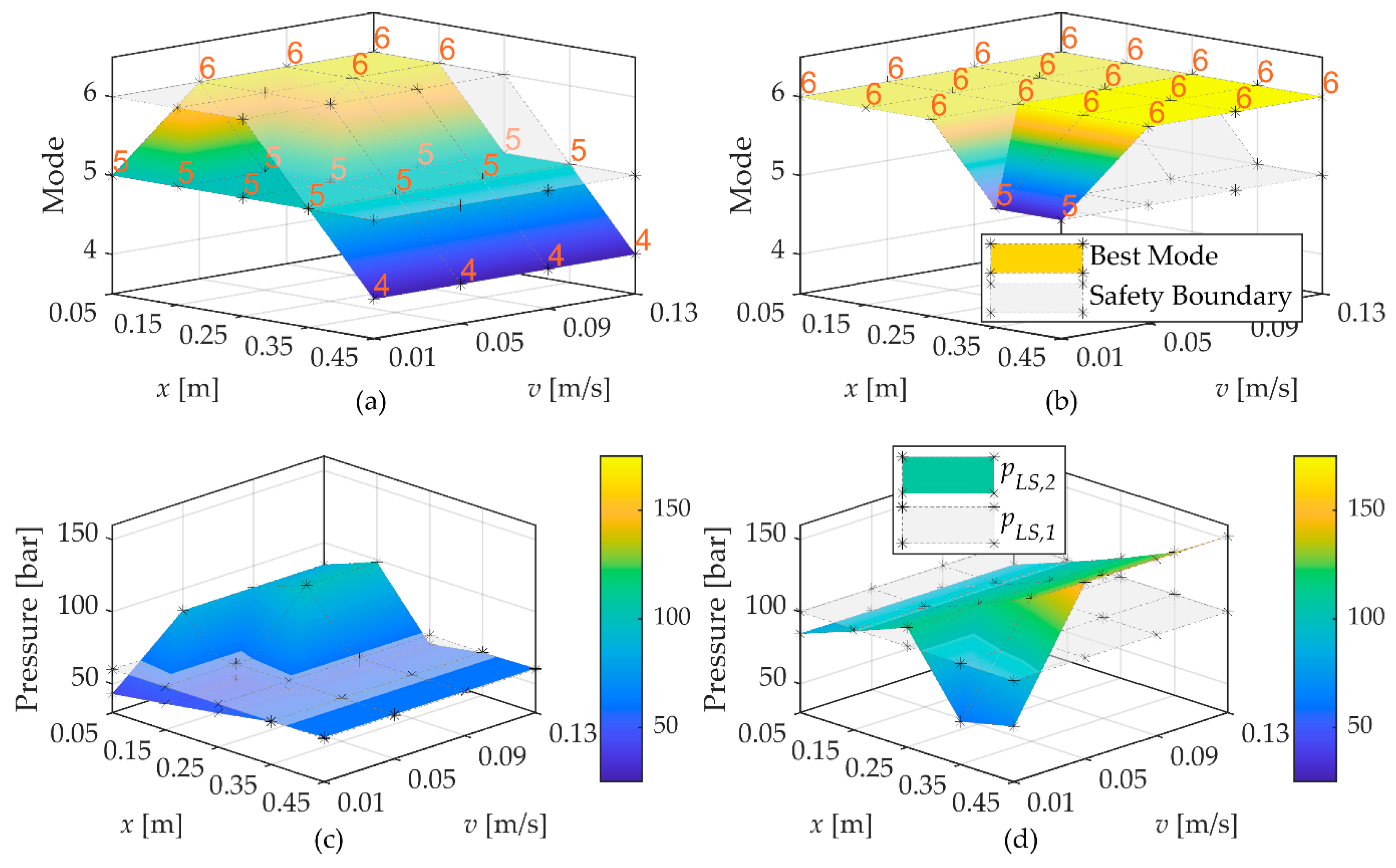
The energy analysis based on the simulation results showed the reduction in energy losses caused by the selection of suitable modes by the agent. However, this does not mean that the training of the agent converged to the global optimal solution that results in the lowest energy losses possible. The optimisation objective has other terms, and, therefore, the results presented in Figure 6 are only an estimation of what are the best modes. Future studies should aim at finding the optimal solution and comparing this with what the agent finds during the training.

The model of the system was judged to be sufficiently accurate to describe the main characteristics and behaviours of the system. Still, there were deviations from the actual behaviour of the system. Although sufficient to pre-train the agent, it is likely that the performance of the agent could be further improved by letting it, in a safe manner, interact with the real system and train from those experiences in order to correct model deviations.

Machine learning-based controllers are a black-box type of controller. There is an inherent risk associated with them when deployed to control real systems, usually related to the controller operating outside the training domain. Therefore, it must be ensured that the control actions applied to the system do not lead to any unsafe and/or unstable behaviours. In this study, this was ensured by implementing safety rules that would overwrite the agent’s decisions when necessary.

One limitation of this study was that the agent was evaluated under approximately the same load conditions and tasks that it was trained for. In the simulation, random noise was introduced to all measurements from the system in order to increase its robustness in the experimental tests. However, there are still questions to be answered and an evaluation to be made regarding the robustness and generalisation capability of the agent. This is especially the case for more realistic load cases, such as digging and variable $p_{LS,1}$ pressure.

6. Conclusions

This paper presents simulation and experimental results that demonstrate the capability of a controller, developed under a reinforcement learning framework, to learn and control the mode selection of a hydraulic system. The controller was trained in simulation and afterwards was deployed to control the real system. The main control objective was to optimise the selection of modes of the multi-chamber actuator so as to reduce the resistive control losses on a valve-controlled load-sensing system. The controller was able to automatically find optimised control decisions and to apply them in the real system. The controller was also shown to be robust to differences between the training domain and the application domain, thus extrapolating the knowledge to unseen situations. Although able to control the real system, the trained agent must be accompanied by safety rules to ensure the safe operation of the system. Future work should be dedicated to evaluating how close the solution is to the global optimum and to assessing its robustness in application, because a high sensitivity to variations in the input features was observed for some of the test cases.

References

1. Vukovic, M.; Leifeld, R.; Murrenhoff, H. Reducing fuel consumption in hydraulic excavators—A comprehensive analysis. Energies 2017, 10, 687. [Google Scholar] [CrossRef] [Green Version]
2. Ketonen, M.; Linjama, M. Simulation study of a digital hydraulic independent metering valve system for an excavator. In Proceedings of the 15th Scandinavian International Conference on Fluid Power, SICFP’17, Linköping, Sweden, 7–9 June 2017. [Google Scholar]
3. Raduenz, H.; Ericson, L.; Heybroek, K.; de Negri, V.J.; Krus, P. Extended analysis of a valve-controlled system with multi-chamber actuator. Int. J. Fluid Power 2021, 23, 79–108. [Google Scholar] [CrossRef]
4. Linjama, M.; Vihtanen, H.; Sipola, A.; Vilenius, M. Secondary controlled multi-chamber hydraulic actuator. In Proceedings of the 11th Scandinavian International Conference on Fluid Power, SICFP09, Linköping, Sweden, 2–4 June 2009. [Google Scholar]
5. Belan, H.C.; Locateli, C.C.; Lantto, B.; Krus, P.; de Negri, V.J. Digital secondary control architecture for aircraft application. In Proceedings of the Seventh Workshop on Digital Fluid Power, Linz, Austria, 26–27 February 2015. [Google Scholar]
6. Dell’Amico, A.; Carlsson, M.; Norlin, E.; Sethson, M. Investigation of a digital hydraulic actuation system on an excavator arm. In Proceedings of the 13th Scandinavian International Conference on Fluid Power SICFP2013, Linköping, Sweden, 3–5 June 2013; pp. 505–511. [Google Scholar] [CrossRef] [Green Version]
7. Huova, M.; Laamanen, A.; Linjama, M. Energy efficiency of three-chamber cylinder with digital valve system. Int. J. Fluid Power 2010, 11, 15–22. [Google Scholar] [CrossRef]
8. Heemskerk, E.; Eisengießer, Z. Control of a semi-binary hydraulic four-chamber cylinder. In Proceedings of the Fourteenth Scandinavian International Conference on Fluid Power, Tampere, Finland, 20–22 May 2015. [Google Scholar]
9. Heybroek, K.; Sjöberg, J. Model predictive control of a hydraulic multichamber Actuator: A feasibility study. IEEE/ASME Trans. Mechatron. 2018, 23, 1393–1403. [Google Scholar] [CrossRef]
10. Donkov, V.H.; Andersen, T.O.; Pedersen, H.C.; Ebbesen, M.K. Application of model predictive control in discrete displacement cylinders to drive a knuckle boom crane. In Proceedings of the 2018 Global Fluid Power Society PhD Symposium (GFPS), Samara, Russia, 18–20 July2018; pp. 408–413. [Google Scholar] [CrossRef]
11. Yuan, H.; Shang, Y.; Vukovic, M.; Wu, S.; Murrenhoff, H.; Jiao, Z. Characteristics of energy efficient switched hydraulic systems. JFPS Int. J. Fluid Power Syst. 2014, 8, 90–98. [Google Scholar] [CrossRef] [Green Version]
12. Vukovic, M.; Murrenhoff, H. Single edge meter out control for mobile machinery. In Proceedings of the ASME/Bath Symposium on Fluid Power & Motion Control, FPMC2014, Bath, UK, 10–12 September 2014. [Google Scholar]
13. Mnih, V.; Kavukcuoglu, K.; Silver, D.; Graves, A.; Antonoglou, I.; Wiersta, D.; Riedmiller, M. Playing Atari with deep reinforcement learning. arXiv 2013, arXiv:1312.5602v1. [Google Scholar]
14. Zhu, Q.; Wang, Q. Real-time energy management controller design for a hybrid excavator using reinforcement learning. J. Zheijang Univ.-Sci. A (Appl. Phys. Eng.) 2017, 18, 855–870. [Google Scholar] [CrossRef]
15. Zhang, W.; Wang, J.; Liu, Y.; Gao, G.; Liang, S.; Ma, H. Reinforcement learning-based intelligent energy management architecture for hybrid construction machinery. Appl. Energy 2020, 275, 115401. [Google Scholar] [CrossRef]
16. Backman, S.; Lindmark, D.; Bodin, K.; Servin, M.; Mörk, J.; Löfgren, H. Continuous control of an underground loader using deep reinforcement learning. Machines 2021, 9, 216. [Google Scholar] [CrossRef]
17. Andersson, J.; Bodin, K.; Lindmark, D.; Servin, M.; Wallin, E. Reinforcement learning control of a forestry crane manipulator. In Proceedings of the 2021 IEEE/RSJ International Conference on Intelligent Robots and Systems (IROS), Prague, Czech Republic, 27 September–1 October 2021. [Google Scholar]
18. Egli, P.; Hutter, M. A general approach for the automation of hydraulic excavator arms using reinforcement learning. IEEE Robot. Autom. Lett. 2022, 7, 5679–5686. [Google Scholar] [CrossRef]
19. Sutton, R.S.; Barto, A.G. Reinforcement Learning—An Introduction, 2nd ed.; MIT Press: Cambridge, MA, USA, 2018; ISBN 9780262039246. [Google Scholar]
20. Berglund, D.; Larsson, N. Controlling a Hydraulic System Using Reinforcement Learning: Implementation and Validation of a DQN-Agent on a Hydraulic Multi-Chamber Cylinder System. Master’s Thesis, Linköping University, Linköping, Sweden, 2021. [Google Scholar]
21. HOPSAN Multi-Domain System Simulation Tool, Division of Fluid and Mechatronic System, Department of Management and Engineering, Linköping University, Linköping, Sweden. Available online: https://liu.se/en/research/hopsan (accessed on 1 June 2022).
22. DQN Agent, Mathworks Reinforcement Learning Toolbox. Available online: https://mathworks.com/help/reinforcement-learning/ug/dqn-agents.html (accessed on 1 June 2022).
Figure 1. Hydraulic-system architecture.
Energies 15 05117 g001
Figure 2. Flow-pressure diagram showing the effect of mode selection on resistive control losses. (a) With a conventional actuator; (b) with a multi-chamber actuator.
Energies 15 05117 g002
Figure 3. Structure of the controller and picture of the test bench.
Energies 15 05117 g003
Figure 4. Agent time step versus system dynamics.
Energies 15 05117 g004
Figure 5. Agent’s training progress.
Energies 15 05117 g005
Figure 6. Best modes for 120 kg load. (a) For p L S , 1 = 60 bar; (b) for p L S , 1 = 100 bar; (c) resultant p L S , 2 for p L S , 1 = 60 bar; (d) resultant p L S , 2 for p L S , 1 = 100 bar.
Energies 15 05117 g006
Figure 7. Simulation result, 40 kg load and p L S , 1 = 60 bar. (a) Position; (b) action; (c) system and load-sensing pressures; (d) power loss.
Energies 15 05117 g007
Figure 8. Simulation result, 40 kg load and p L S , 1 = 100 bar. (a) Position; (b) action; (c) system and load-sensing pressures; (d) power loss.
Energies 15 05117 g008
Figure 9. Energy comparison, p L S , 1 = 60 bar: (a) 40 kg; (b) 80 kg; (c) 120 kg; (d) 160 kg; (e) 200 kg; (f) 240 kg.
Energies 15 05117 g009
Figure 10. Energy comparison, p L S , 1 = 100 bar: (a) 40 kg; (b) 80 kg; (c) 120 kg; (d) 160 kg; (e) 200 kg; (f) 240 kg.
Energies 15 05117 g010
Figure 11. Experimental (Test) and simulation (Sim) results, 40 kg load and p L S , 1 = 60 bar. (a) position and reference; (b) action; (c) system pressure.
Energies 15 05117 g011
Figure 12. Experimental (Test) and simulation (Sim) results, 40 kg load and p L S , 1 = 100 bar. (a) Position and reference; (b) action; (c) system pressure.
Energies 15 05117 g012
Figure 13. All test cases, p L S , 1 = 60 bar: (a) 40 kg; (b) 80 kg; (c) 120 kg; (d) 160 kg; (e) 200 kg; (f) 240 kg.
Energies 15 05117 g013
Figure 14. All test cases, p L S , 1 = 100 bar: (a) 40 kg; (b) 80 kg; (c) 120 kg; (d) 160 kg; (e) 200 kg; (f) 240 kg.
Energies 15 05117 g014
Figure 15. Issues with repeatability for 120 kg load and p L S , 1 = 60 bar.
Energies 15 05117 g015