Multi-Level Dependent-Chance Model for Hydropower Reservoir Operations

Abstract

Some hydropower reservoirs are operated under different constraint levels. For these reservoirs, a multi-level (ML) dependent-chance (DC) model is established. In the model, only when the higher-level constraints are satisfied are the lower-level constraints or system benefits considered. The multi-level dependent-chance (MLDC) model is specified by two models. One is based on existing reliability-constrained (RC) dynamic programming (DP), in which the soft constraints are addressed using reliability constraints of 1, and the priorities are reflected using the order of magnitudes of Lagrange multipliers. The other is the explicit dependent-chance reasoning in the DP recursive function, in which each soft constraint is represented as an objective function of negative expected failure time and the optimum is the solution with a larger value for all higher-level objective functions. The proposed models are applied to derive long-term operation rules for the hydropower system on the middle-lower Lancang River. The results show the feasibility and performances of the explicit graded constraint control of the proposed model and the solution methods.

1. Introduction

Reservoir operations are central to our ability to manage river basin systems serving conflicting multi-sectoral demands under increasingly uncertain futures. Real-world hydropower reservoir operations are very complex, with stochastic inputs (inflows and demands), nonlinear system dynamics (the release decision depends on the product of the release and the storage level), feedbacks (immediate and future consequences are interdependent), as well as imprecise secondary operating objectives (environmental, flood control, etc.) [1]. Methods including linear programming (LP), dynamic programming (DP), nonlinear programming (NLP), and simulation have been used in the optimization of reservoir operations [2,3,4]. The operation of hydropower reservoirs needs to follow energy generation rules [5,6,7] to increase benefit, and must consider the criteria of reliability, resiliency, and vulnerability [8]. In a centralized operated power system with no time-varying energy price, the economic benefit is often evaluated using the amount of energy generation, and bounds on power generation and reservoir release are set to be constraints. Due to the stochastic inflow, there may be no feasible solution when they are addressed as hard constraints, so the constraints are all soft constraints [9], chance constraints, or reliability constraints [10,11,12,13,14].

Due to the uncertainty of the inflow [15,16,17], long-term reservoir operations are stochastic programming problems, and stochastic dynamic programming [18,19] is one of the most popular methods for long-term hydropower reservoir operations under uncertain inflows. To solve the challenges of the curse of dimensionality, the curse of modeling, and the curse of multiple objectives [20] of SDP in complex real-world water resource problems, improvements such as sampling stochastic dynamic programming [21], the aggregation–disaggregation approach [22], aggregate SDP [23], stochastic dual dynamic programming (SDDP) [24], reinforcement learning [25], and simulation-optimization methods [26,27] were proposed. In the methods, to address the soft constraints on power generation, reservoir release is an important factor that impacts the solution quality.

The SDP models are used to derive operation rules in infinite time horizons or obtain operation policy in finite time horizons [28] for benefit maximization. The benefits of hydropower reservoirs come mostly from energy generation, and the bounds or targets of release and power generation are often formulated as soft constraints. In SDP, the soft constraints can be addressed using penalty functions. Tejada-Guibert et al. [29,30] used two penalty terms in the benefit function of energy value maximization to address water target shortfalls and power target shortfalls. Tilmant and Kelman [31] presented a methodology for analyzing trade-offs and risks associated with large-scale water resource projects under hydrologic uncertainty based on SDDP, in which the immediate cost function includes generation costs and the penalties for not meeting operating targets and/or violating operating constraints, such as energy demand. Marques and Tilmant [9] penalized deviation from given target operations (violations of constraints) such as energy deficit, environmental flows, spills, and other water demands in the SDDP model for coordination in large-scale multi-reservoir systems. Kim et al. [32] proposed optimizing operational policies of a multi-reservoir system using SSDP with ensemble streamflow prediction, in which the demands of minimizing water shortages, minimizing the difference between the firm water supply elevation and the actual, and energy productions are combined into an objective function. The penalty-based methods can address multiple soft constraints by adding several terms to the objective function, but encounter problems of balance among penalty terms and between the penalty and objective, and the performance of the obtained policy depends on the form and coefficients used in the penalty terms. Thus, the penalty function is not always effective for reservoir operation models. For example, Quinn et al. [33] studied the reservoir operation problem for the Red River basin with multi-objectives of hydropower production, agricultural water supply, and flood protection, and found that minimizing flood damage in expectation may be ill-advised because it is difficult to know a priori whether or not doing so will be effective in reducing severe floods, especially when damages are uncertain or nonstationary and need to be approximated by a nonlinear penalty function.

Another alternative to address soft constraints is using explicit chance-constrained approaches. Askew et al. [10] proposed chance-constrained dynamic programming (CCDP), in which the iterative search of a penalty for failure and a precise evaluation of the response of the system may be carried out within the dynamic program by means of minor additions to its basic algorithm. Rossman [11] presented an SDP model for determining reservoir release rules subject to reliability constraints on system performance within the framework of Lagrangian duality theory. Sniedovich [12] developed a dynamic programming solution procedure for a class of reliability-constrained reservoir control problems associated with constraints defined over the entire life of the reservoir. The chance-constrained methods need preset reliability levels on different constraints. This may be difficult until the model is solved using different tested reliability values. The reliabilities on different constraints may conflict with each other.

There can be multiple demands, economic benefits [34], or noneconomic requirements [35,36,37] for hydropower reservoir operations. For some hydropower reservoir systems, the demands may have explicit priorities. The trade-off between noneconomic requirements is often factitious. In the penalty function-based method, it depends on penalty coefficients and exponents for different terms, while in reliability-constrained models, it depends on demanded chance values for different constraints and the solution method. The magnitudes of coefficients or chance values can partly reflect the priorities of different constraints, but the constraints interact for numerical reasons in the solution so that for problems with multiple soft constraints with different priorities, the priorities may not be fully reflected.

In this paper, a multi-level dependent-chance (MLDC) problem for reservoir operations is presented to address multiple interconnected soft constraints. Two specific models for MLDC problems are proposed. The first model solves the MLDC model based on reliability-constrained dynamic programming (RCDP), in which all soft constraints are replaced by chance constraints set at 1, and the priorities of the constraints are reflected by presetting Lagrange multipliers for different level constraints. The second model is the explicit dependent-chance dynamic programming (DCDP)-based model, in which the constraint priorities are reflected in DP recursive functions. In the DCDP model, all of the soft constraints and benefits are formulated as objectives with different priorities, and the benefit functions in common dynamic programming (DP) are replaced by a vector of the objectives. The criterion of benefit maximization in the solution at each state is replaced by comparing the logic that better performances of objectives with higher priorities is better. Both models can use inflow probability distributions and inflow samplings, and accordingly, MLRC-SDP, MLRC-SSDP, MLDC-SDP, and MLDC-SSDP are used to solve the multi-level constrained reservoir operation model, with the first two an extension of single-level RCDP and the last two being newly proposed. The proposed models are used with a single reservoir and a cascaded reservoir system on the middle-lower Lancang River in China, taking minimum release, extreme minimum power, and firm power as three level constraints, and energy maximization as the benefit objective. The results show the performances of the proposed method in the solution.

2. Materials and Methods

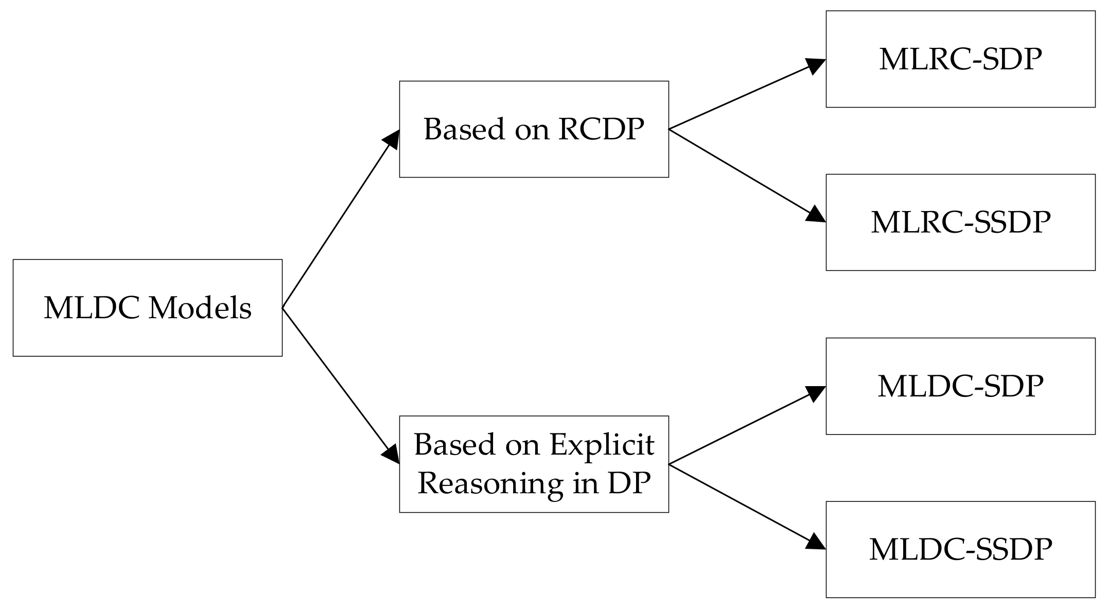
In this section, four reservoir operation models are proposed: MLRC-SDP, MLRC-SSDP, MLDC-SDP, and MLDC-SSDP. Moreover, Figure 1 illustrates these four reservoir operation models.

2.1. Multi-Level Dependent-Chance Reservoir Operation Model

In hydropower reservoir operation models, there are constraints on reservoir storage, release, and power generation. Constraints on storage can be satisfied by confining the discretized storage values, while the constraints on minimum release and power generation are soft constraints, essentially. In real operations, the constraints often have clear priorities, and the constraints with higher priorities need to be satisfied at the cost of low-level constraints failing and loss of economic benefit. The operation for this kind of reservoir can be summarized as to satisfy the highest-level constraint as far as possible, then satisfy lower-level constraints as far as possible without increasing the probability of failing to meet all higher-level constraints, then maximize the economic objective without increasing the probability of failing to meet the constraints of any level. For example, a hydropower reservoir is operated to satisfy a minimum release for ecological, environmental, or shipping requirements, an extreme minimum power in extreme dry periods, a designed firm power, and to maximize the energy generation. Although the soft constraints can be addressed using penalty functions or reliability-constrained models, the demands of satisfying constraints strictly following the priorities need to be formulated as new models.

Liu [38,39] proposed a type of stochastic programming paralleled to the expected value model and chance-constrained programming, named dependent-chance programming (DCP). In DCP, the objectives are to maximize or minimize the probabilities of certain events. Supposing that a reservoir system has J level of constraints, and the constraints are sorted according to the priority as 1:J, together with the benefit objective, there are J + 1 levels of objectives. Following DCP, the objectives for the soft constraints of the studied reservoir operation model are as Equation (1), and the objective for energy maximization is as Equation (2).

$$\mathit{max} F_j\left(p_t^m,r_t^m\right)=\mathrm{Pr}\left[g_j\left(p_t^m,r_t^m\right)\ge 0, m =1:M, t =1:T\right], j=1:J$$

(1)

$$\mathit{max} F_{J+1}\left(p_t^m,r_t^m\right)={\displaystyle \sum }_{t=1}^T{\displaystyle \sum }_{m=1}^M{p}_t^m{\mathsf{\Delta }}_t$$

(2)

where m, t, and j are sequence numbers of reservoirs, periods, and soft constraints, and M, T, and J are the total numbers; $F_j\left(p_t^m,r_t^m\right), j=1:J+1$, is the jth objective function; $g_j\left(p_t^m,r_t^m\right)$, j = 1:J, is the jth soft constraint about power generation $p_t^m$ and release $r_t^m$; and ${\mathsf{\Delta }}_t$ is the hour number in period t.

The model formulated as Equations (1) and (2) is a multi-objective model. For the soft constraints with explicit priorities, the objective functions of Equations (1) and (2) can be replaced by the objective function of MLDC as Equation (3), in which the objective for a higher-level demand is optimized in a feasible region where all lower-level objectives take the optimal values.

$$F_j^{*}=\underset{F_i=F_i^{*},i=1:j-1}{max} \left[F_j\left(p_t^m,r_t^m\right)\right] , j=1:J+1$$

(3)

where $F_i^{*}$ is the optimal solution for the ith-level objective.

Equation (3) means that a lower-level objective $F_j\left(p_t^m,r_t^m\right)$ can only be optimized in the region where all higher-level objectives obtain the optimal values.

2.2. MLDC Model Based on RCDP

RCDP [11] can solve the models with chance constraints. For an energy maximization model with J soft constraint of the multi-reservoir system, the jth reliability constraint is Equation (4).

$$\mathrm{Pr}\left[g_j\left(p_t^m,r_t^m\right)\ge 0\right]\ge {\gamma }_j, j=1:J$$

(4)

where ${\gamma }_j$ is the constrained value for the jth reliability constraint.

To solve the reliability-constrained model using DP, the recursive function is formulated as Equation (5) at period t and state k.

$$f_t^{opt}\left(S_t^k\right)=\underset{R_t^k}{\max }{\displaystyle \sum }_{n=1}^{N}P{r}_t\left(n\right)\left\{B_t\left(R_t^k,Q_t^n,S_t^k\right)+{\displaystyle \sum }_{j=1}^J{\lambda }_j\left[L_j\left(R_t^k,Q_t^n,S_t^k\right)-{\gamma }_j\right]+f_{t+1}^{opt}\left(S_{t+1}\right)\right\}$$

(5)

where $L_j\left(R_t^k,Q_t^n,S_t^k\right)=\left\{\begin{array}{c}0 g_j\left(R_t^k,Q_t^n,S_t^k\right)<0\\ 1 g_j\left(R_t^k,Q_t^n,S_t^k\right)\ge 0\end{array}\right.$, $B_t\left(R_t^k,Q_t^n,S_t^k\right)$ is the benefit function; $g_j\left(R_t^k,Q_t^n,S_t^k\right)\ge 0$ is the jth soft constraint; N is the combination number of discretized reservoir inflow scenarios; $f_t^{opt}\left(S_t^k\right)$ is the optimal Lagrange terms augmented objective value at the beginning of period t at state $S_t^k$; $f_{t+1}^{opt}\left(S_{t+1}\right)$ is the future value at the beginning of period t + 1 at storage vector $S_{t+1}$; $P{r}_t\left(n\right)$ is the probability of $Q_t^n$; and ${\lambda }_j$ is the Lagrange multiplier for the jth constraint. $S_t^k=\left(s_t^{k,1},s_t^{k,2},\cdots ,s_t^{k,M}\right)$ is the vector of the kth discrete storage combination at period t, and the number of discretized state combinations is K at period t; $s_t^{k,m}$ is the storage of reservoir m in $S_t^k$; $R_t^k=\left(r_t^{k,1},r_t^{k,2},\cdots ,r_t^{k,M}\right)$ is the vector of the release decision combination at the state of $S_t^k$; $Q_t^n=\left(q_t^{n,1},q_t^{n,2},\cdots ,q_t^{n,M}\right)$ is the vector of the nth discrete local inflow combination at period t; and $q_t^{n,m}$ is the local inflow of reservoir m in $Q_t^n$.

The state transition function from $S_t^k$ to $S_{t+1}$ is the water balance functions of $s_{t+1}^m=s_t^{k,m}+q_t^{n,m}+{{\displaystyle \sum }}_{i=1}^{u_m}{r}_t^{k,i}-r_t^{k,m}$, considering reservoir storage bounds, and for all reservoirs, $u_m$ is the number of immediate upstream reservoirs of reservoir m.

In the reliability-constrained model, ${\gamma }_j$ is known, and the values of ${\lambda }_j$ need to be computed iteratively. In DCP models, ${\gamma }_j$ is unknown. To precisely solve the model of Equation (2), both of the values of ${\gamma }_j$ and ${\lambda }_j$ need to be computed iteratively. The values of ${\gamma }_j$ are difficult to set for each lower-level chance constraint; the maximum probability that can be reached in a region depends on high-level constraints, following the definition of the priority level. Hence, the chance value for the highest-level constraint must be calculated first, neglecting the other chance constraints, and the chance constraint for the highest level must be fixed to calculate the constraint value for the second-highest-level constraint, until the lowest level. In each step, the inter-affected ${\lambda }_j$ has to be solved iteratively. Thus, the solution can be very complex and time consuming.

Fortunately, the solution method can be simplified. If the demand is to satisfy the constraints as far as possible, all of the ${\gamma }_j$ can be set to be 1. According to the reliability-constrained models, there may be no solution when all ${\gamma }_{j }=1$, so the ${\lambda }_j$ needs not be valued iteratively, and different level values of ${\lambda }_j$ can be set to reflect the priority of the soft constraints and the model can be solve using DP. This is an approximate solution method to the MLDC model, for the ${\lambda }_j$ values control the result.

Considering space and time inflow correlations [21,40], the recursive function can be transformed into Equations (6) and (7).

$$f_t^{opt}\left(S_t^k\right)=\underset{R_t^k}{max}{\displaystyle \sum }_{d=1}^D\frac{1}{D}\left\{B_t^d\left(R_t^k,S_t^k\right)+{\displaystyle \sum }_{j=1}^J{\lambda }_j\left[L_j^d\left(R_t^k,S_t^k\right)-{\gamma }_j\right]+F_{t+1}{}^d\left(S_{t+1}\right)\right\}$$

(6)

$$F_{t+1}{}^d\left(S_{t+1}\right)=\left\{\begin{array}{l}{f}_{t+1}^{opt,d}\left(S_{t+1}\right)t\ne T\\ \frac{1}{D}{\displaystyle {\displaystyle \sum }_{d0=1}^D}{f}_{t+1}^{opt,d0}\left(S_{t+1}\right) t=T\end{array}\right.$$

(7)

where D is the inflow sampling number, and $B_t^d\left(R_t^k,S_t^k\right)$ and $f_{t+1}^{opt,d}\left(S_{t+1}\right)$ are the benefit function and the future value function of the inflow sample m, respectively.

The model of Equation (5) can be called MLRC-SDP and the model of Equations (6) and (7) can be called MLRC-SSDP.

2.3. MLDC Model Based on Explicit Reasoning in DP

To precisely solve the MLDC model, an MLDC-SDP model is proposed. In the MLDC-SDP model, whether a soft constraint is satisfied or not is formulated as objectives with values of 0, −1. The probability maximization for the jth soft constraint is as Equation (8) with $1\le j\le J$, and the corresponding objective function used in computation is as Equation (9).

$$max \mathrm{Pr}\left[g_j\left(R_t^k,Q_t^n,S_t^k\right)\ge 0\right]$$

(8)

$$B_{j,t}\left(R_t^k,Q_t^n,S_t^k\right)=\left\{\begin{array}{l}-1g_j\left(R_t^k,Q_t^n,S_t^k\right)<0\\ 0 \mathrm{otherwise}\end{array}\right.$$

(9)

where $B_{j,t}\left(R_t^k,Q_t^n,S_t^k\right)$ is the objective of the reservoir for satisfying constraint j at period t.

Following Equation (3), the operation of the reservoir has to satisfy the first-level constraint (j = 1 in Equation (3)) as far as possible, and the recursive function for this objective is Equation (10).

$$f_{j,t}^{opt}\left(S_t^k\right)=\underset{R_t^k}{\max }{\displaystyle \sum }_{n=1}^{N}P{r}_t\left(n\right)\left[B_{j,t}\left(R_t^k,Q_t^n,S_t^k\right)+f_{j,t+1}^{opt}\left(S_{t+1}\right)\right], j=1$$

(10)

where $f_{j,t}^{opt}\left(S_t^k\right)$ is the optimal expected time of reservoirs satisfying constraint j from period t at state $S_t^k$. $g_j\left(R_t^k,Q_t^n,S_t^k\right)$ and $B_{j,t}\left(R_t^k,Q_t^n,S_t^k\right)$ are decided by real release and final storage when trying to release $R_t^k$ at $S_t^k$.

Following Equation (8), there is no difference between the policies that have the same chance of satisfying the first-level constraint. Considering the other objectives, the optimal decisions have to be confined to the regions with the maximum value of the first-level objective. To include other objectives, the condition has to be introduced into lower-level recursive functions to confine the feasible region. For the second-level constraint, the recursive function is Equation (11).

$$f_{j,t}^{opt}\left(S_t^k\right)=\underset{R_t^k,f_{j-1,t}^{R_t^k}\left(S_t^k\right)=f_{j-1,t}^{opt}\left(S_t^k\right)}{\max }{\displaystyle \sum }_{n=1}^{N}P{r}_t\left(n\right)\left[B_{j,t}\left(R_t^k,Q_t^n,S_t^k\right)+f_{j,t+1}^{opt}\left(S_{t+1}\right)\right],j=2$$

(11)

where $f_{j,t}^{R_t^k}\left(S_t^k\right)$ is the objective value for the jth objective at period t, given state $S_t^k$ and decision $R_t^k$.

Different from Equation (10), the $R_t^k$ is confined to the region of $f_{j-1,t}^{R_t^k}\left(S_t^k\right)=f_{j-1,t}^{opt}\left(S_t^k\right)$. This means that only the decisions whose first-level objective values are equal to the optimum can be selected as the solution. Thus, for the operating policy following Equation (11), the objective of constraint level 1 is fixed at the maximum value. Under this condition, the objective of constraint 2 is maximized.

The recursive function for other level constraints is similar. This way, $f_{j,t}^{opt}\left(S_t^k\right)$ for each level of constraint can be obtained in turn of j = 1:J, through maximizing a lower-level objective in the condition of not decreasing all of the higher-level objectives. Considering all levels of objectives, the final recursive function is Equation (12).

$$f_{j+1,t}^{opt}\left(S_t^k\right)=\underset{R_t^k,f_{j,t}^{R_t^k}\left(S_t^k\right)=f_{j,t}^{opt}\left(S_t^k\right),j=1:J}{\max }{\displaystyle \sum }_{n=1}^{N}P{r}_t\left(n\right)\left[B_{j+1,t}\left(R_t^k,Q_t^n,S_t^k\right)+f_{j+1,t+1}^{opt}\left(S_{t+1}\right)\right]$$

(12)

where the $B_{j+1,t}\left(R_t^k,Q_t^n,S_t^k\right)$ is the objective function of energy generation. The confines of the feasible region mean that the optimal release decision has to be selected from the region with optimal values for all constraint levels.

Considering the space and time inflow correlations, an SSDP version of the MLDC-SDP (MLDC-SSDP) is as Equations (13) and (14).

$$f_{j+1,t}^{opt}\left(S_t^k\right)=\underset{\begin{array}{c}{R}_t{}^k,f_{j,t}^{R_t^k}\left(S_t^k\right)=\\ f_{j,t}^{opt}\left(S_t^k\right),j=1:J\end{array}}{max}{\displaystyle \sum }_{d=1}^D\left[B_{j+1,t}^d\left(R_t^k,S_t^k\right)+F_{j+1,t+1}{}^d\left(S_{t+1}\right)\right]$$

(13)

$$F_{j+1,t+1}{}^d\left(S_{t+1}\right)=\left\{\begin{array}{l}{f}_{j+1,t+1}^{opt,d}\left(S_{t+1}\right) t\ne T\\ \frac{1}{D}{\displaystyle {\displaystyle \sum }_{d0=1}^D}{f}_{j+1,t+1}^{opt,d0}\left(S_{t+1}\right) t=T\end{array}\right.$$

(14)

where $B_{j,t}^d\left(R_t^k,S_t^k\right)$ and $f_{j,t+1}^{opt,d}\left(S_{t+1}\right)$ are the benefit function and the future value function of the inflow sample d for objective level j, respectively.

2.4. Solution Algorithm

All of the Lagrange terms for soft constraints are merged into one objective function, so the solution algorithm for MLRC-SDP and MLRC-SSDP is the same as those for common SDP models, while the solution algorithm to MLDC-SDP and MLDC-SSDP needs to be illustrated. The following solving algorithm takes the MLDC-SDP as an example, and the MLDC-SSDP can be solved using a similar method.

Following the basic solution method of SDP in the infinite horizon, the boundary condition for all objective functions, $f_{j,T+1}^{opt}$, is set to 0 for the last period, and the decision is solved from the last period backward through period 1 in one round iteration on the time horizon. If the decision at all states is same to the last round of iterations, a stable operating rule is obtained, or another round is repeated after replacing $f_{j,T+1}^{opt}$ with $f_{j,1}^{opt}$.

At each state of $S_t^k$, the optimization problem is to find the optimal $R_t^k$ according to the predefined objective functions and the priorities of them. Following Equations (3) and (12), the optimal problem can be described as Equation (15):

$$\underset{R_t^k}{Max} f_{j+1,t}^{R_t^k}\left(S_t^k\right)|f_{j,t}^{R_t^k}\left(S_t^k\right)=\left\{f_{j,t}^{opt}\left(S_t^k\right)|\left[f_{j-1,t}^{R_t^k}\left(S_t^k\right)=\left(f_{j-1,t}^{opt}\left(S_t^k\right)|\cdots f_{1,t}^{R_t^k}\left(S_t^k\right)=f_{1,t}^{opt}\left(S_t^k\right)\right)\right]\right\}$$

(15)

In fact, the solution need not use several steps, and each step can solve the optimization model for one level objective, as Equation (13) denotes. The optimal solution can be obtained considering all level objectives with priorities in one step, given a new logic comparing the solutions to replace the objective value in the common SDP. The objective values for a discrete decision can be formulated as a vector of $G_m=\left\{g_{1,i},g_{2,i},\cdots ,g_{J+1,i}\right\}$, $g_{j,i}$, j = 1:J + 1, is the jth level objective of the ith discrete decision. The problem of searching for the solution with largest benefit value in the common SDP is changed to search for the best solution according to a comparing logic that considers all levels of constraints and benefits. The comparing logic is as follows: $G_1=G_2$ means that all of the objective values of the two decisions are equal, and $G_1>G_2$ means that there exists a level, j; for all higher levels than j, the objective values in $G_1$ and $G_2$ are equal, and at level j, the objective value in $G_1$ is larger than in $G_2$. This can be formulated as $g_{1,1}>g_{1,2}\vee \left(g_{1,1}=g_{1,2}\wedge g_{2,1}>g_{2,2}\right)\vee \cdots \vee \left(g_{1,1}=g_{1,2}\wedge g_{2,1}=g_{2,2}\wedge \cdots \wedge g_{J,1}=g_{J,2}\wedge g_{J+1,1}>g_{J+1,2}\right)$. 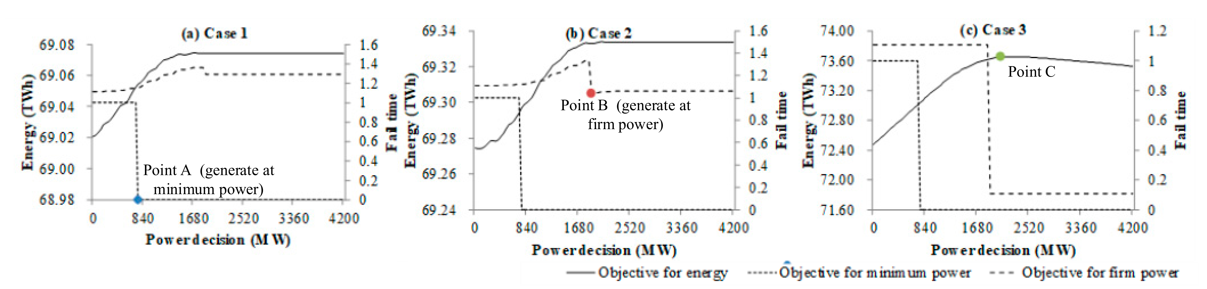Figure 2 denotes the solution for an example of the MLDC-SDP for energy maximization with two levels of constraints on minimum power and firm power. In Figure 2a,b, the optimal solutions are the powers according to point A and B, and the single decisions with minimum expected firm power failing times in the regions where the expected minimum power failing times are 0. In Figure 2c, the optimal solution is the power according to point C, with the largest expected energy in the region where the expected failing times for both minimum power and firm power are minimum.

In the solution, the objective values of the two decisions are compared from the highest level to the lowest level. If, at any level, all of the higher-level benefit values are equal, the decision with a larger current level objective value is better than the others. Different from the solution of the standard SDP, there are J + 1 future value functions for each period. Each future value function $f_{j,t+1}^{opt}\left(S_{t+1}\right)$ value can be obtained by fitting the surface near the point of $S_{t+1}$ using the points around it. For one reservoir problem, linear interpolation is used, and for two reservoir problems, the fitting function of $f_{j,t+1}^{opt}\left[\left(s_{t+1}^1,s_{t+1}^2\right)\right]=a{s}_{t+1}^1+b{s}_{t+1}^2+c{s}_{t+1}^1{s}_{t+1}^2+d$ is used.

Unlike concave maximization reservoir operation models [41,42], a hydropower operation problem for a single decision may not be concave for water head varying and may have more than one local optimization [43]. The objective functions for satisfying soft constraints are probability weighted as 0 or −1, so there are rapid value changing regions in the objective function. The confines on feasible regions of the benefit function caused by soft constraints can result in the benefit function having several increasing–decreasing fluctuations. Thus, considering all level objectives, there can be several local optima, and the solution algorithm has to search the whole feasible region of $R_t^k$ to ensure local optima are not missed. The $r_t^{k,m}$, $m=1,2,\cdots ,M$, is valuated among C discrete values; there are $C^M$ decisions [44], and the best among them is found through comparing all of the discrete decisions. This solution approach is called traversing [45]. Through traversing, both an optimal decision and the other local optimization in the discretized decisions can be found. To increase the solution accuracy, better solutions can be found near all of the local optima after traversing, using local search algorithms [37,45,46]. In the local search stage of this paper, regions near each local optimum are searched continuously using a searching step until no better solution is found, and then the searching step is halved and the searching is repeated for several times until the search step is small enough. In some cases, the new, better solution near the optimal decision obtained by traversing is still better than the new solutions near the other local optima. However, it is not absolute, and it is also possible that the best solution can be found in a local search region near other local optima besides the best solution from traversing. More details can be referred to in Wu et al. [45].

3. Case Study

3.1. Cascaded Hydropower Reservoirs on Lancang River

The Lancang River is an international river, and outside of China it is known as the Mekong River. The Lancang–Mekong River is about 4900 km long, and it flows through China, Myanmar, Laos, Thailand, Cambodia, and Vietnam, before flowing into the South China Sea. Within China, it is about 2100 km long and has a drainage area of about 174,000 km². The hydropower system studied in this paper is located in the middle and lower reaches of the Lancang River in Yunnan Province. The studied system in this paper consists of five hydropower reservoirs with a total installed capacity of 14,820 MW. The structure of the stated hydropower system is shown in Figure 3, and the characteristics of the hydropower reservoirs are shown in

Table 1. Characters of hydropower reservoirs on main stream of Lancang River in Yunnan Province.

Reservoirs	Drainage Area (104 km2)	Average Local Inflow (m3s−1)	Installed Capacity (MW)	Beneficial Storage (108 m3)
Xiaowan	11.33	1234	4200	98.77
Manwan	11.45	13	1670	2.57
Dachaoshan	12.10	106	1350	3.70
Nuozhadu	14.47	394	5850	113.35
Jinghong	14.91	53	1750	3.09

. The reservoirs of Xiaowan and Nuozhadu have a large reservoir capacity, and the operating rules of them are to be optimized, while the other reservoirs are assumed to be run-of-river. Historical inflow data from 1953 to 2008 are used in this study. The reservoir storage is discretized into 51 points. The inflows of each month are divided into five intervals to obtain discretized probability distributions in the SDP models, and all of the 56 yearly inflows are used as inflow samples in the SSDP models.

3.2. Single Reservoir Case Study

The Xiaowan reservoir (numbered 1), located in the middle stream of the Lancang River, is a multi-year regulating storage reservoir. The constraints on the Xiaowan reservoir are set as three levels in this case study: $r_t^1\ge \underset{\_}{r}$, $\underset{\_}{r}$ = 470 m³s⁻¹ is the minimum outflow;$p_t^1\ge \underset{\_}{p}$, $\underset{\_}{p}$ is a minimum power; $p_t^1\ge fp$, fp = 1854 MW is the firm power. The power generation is set as the decision variable. The four models of MLRC-SDP, MLRC-SSDP, MLDC-SDP, and MLDC-SSDP are applied to the reservoir.

There is no coefficient in MLDC-SDP and MLDC-SSDP. For MLRC-SDP and MLRC-SSDP, the constraints of reliabilities and coefficients cannot be decided before time-consuming iterative computation. For simplicity, the constraints of reliabilities on firm power, minimum power, and minimum release are set to be ${\gamma }_j=1$, j = 1, 2, 3 in Equation (2), and the priorities of the constraints are reflected by the values of coefficients by setting ${\lambda }_1=1\times {10}^{10}$, ${\lambda }_2=1\times {10}^{20}$, and ${\lambda }_3=1\times {10}^{30}$.

Table 2. Computing results for single reservoir of Xiaowan.

Minimum Power Setting	Model	Energy (TWh)	Reliability on Firm Power (%)	Reliability on Minimum Power (%)
60% of firm power	MLDC-SDP	1083.6	96.4	100
	MLDC-SSDP	1086.5	95.5	100
	MLRC-SDP	1083.8	96.7	99.9
	MLRC-SSDP	1087.5	94.5	100
90% of firm power	MLDC-SDP	1104.3	39.7	97.5
	MLDC-SSDP	1099.1	59.7	100
	MLRC-SDP	1103.4	52.9	96.1
	MLRC-SSDP	1097.4	60.9	100

shows the computing results using a minimum power of ${\underset{\_}{p}}_1=60\%fp$ and ${\underset{\_}{p}}_2=90\%fp$. The $\underset{\_}{r}$ constraints are satisfied at all periods using all methods. In Table 2, the energy generation for $\underset{\_}{p}={\underset{\_}{p}}_1$ is smaller than $\underset{\_}{p}={\underset{\_}{p}}_2$ using all solution methods. This is because the constraint of $\underset{\_}{p}={\underset{\_}{p}}_1$ is easily satisfied and the reservoir needs try to satisfy the fp constraint in most periods, while the ${\underset{\_}{p}}_2$ is close to fp and is much harder to satisfy than ${\underset{\_}{p}}_1$, so the reservoir must satisfy ${\underset{\_}{p}}_2$ in most periods. Hence, the constraint affect decisions in most periods is increased from ${\underset{\_}{p}}_1$ to ${\underset{\_}{p}}_2$.

For the MLDC model preferentially optimizing the probabilities of satisfying higher-level constraints, the solution quality can be evaluated by comparing the reliability on $\underset{\_}{r}$, reliability on $\underset{\_}{p}$, reliability on fp, and energy generation in turn. If the $\underset{\_}{r}$ constraint is satisfied at all periods, the solution with the largest reliability on $\underset{\_}{p}$ is the best. From Table 2, it can be seen that when $\underset{\_}{p}={\underset{\_}{p}}_1$, the results of the solutions are close to each other. When $\underset{\_}{p}$ is a much larger value of ${\underset{\_}{p}}_2$, the reliability on $\underset{\_}{p}$ can be 2.5% larger comparing MLDC-SSDP to MLDC-SDP, and 3.9% larger comparing MLRC-SSDP to MLRC-SDP, and the reliability on fp is much larger for the SSDP models compared to the SDP models. This indicates that when a higher-level constraint is easily satisfied, the inflow temporal correlation may not impact the simulation results significantly for large reservoirs, while when the higher-level constraint is more difficult to satisfy, the inflow temporal correlations are an important factor to estimate the failing chance.

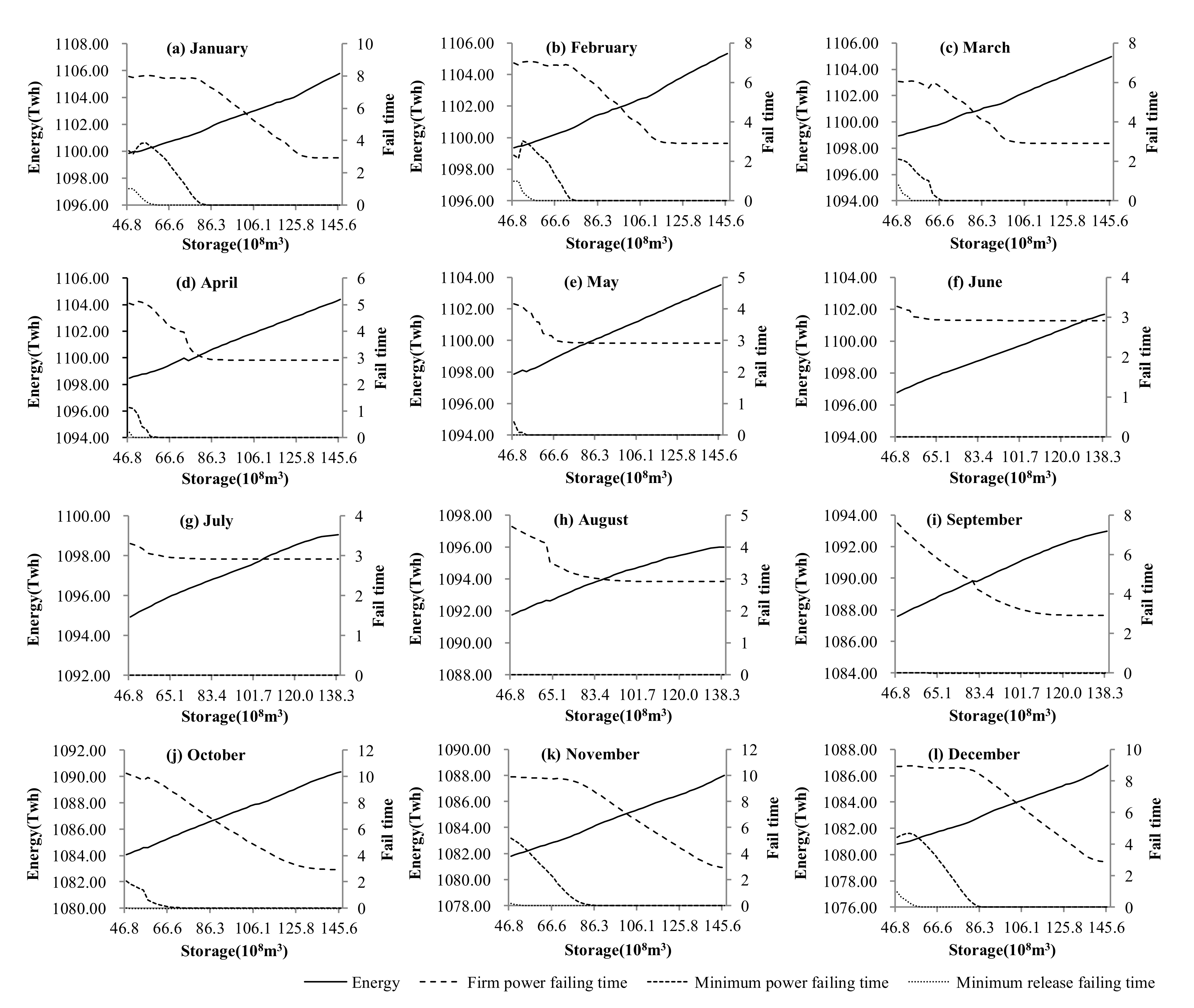
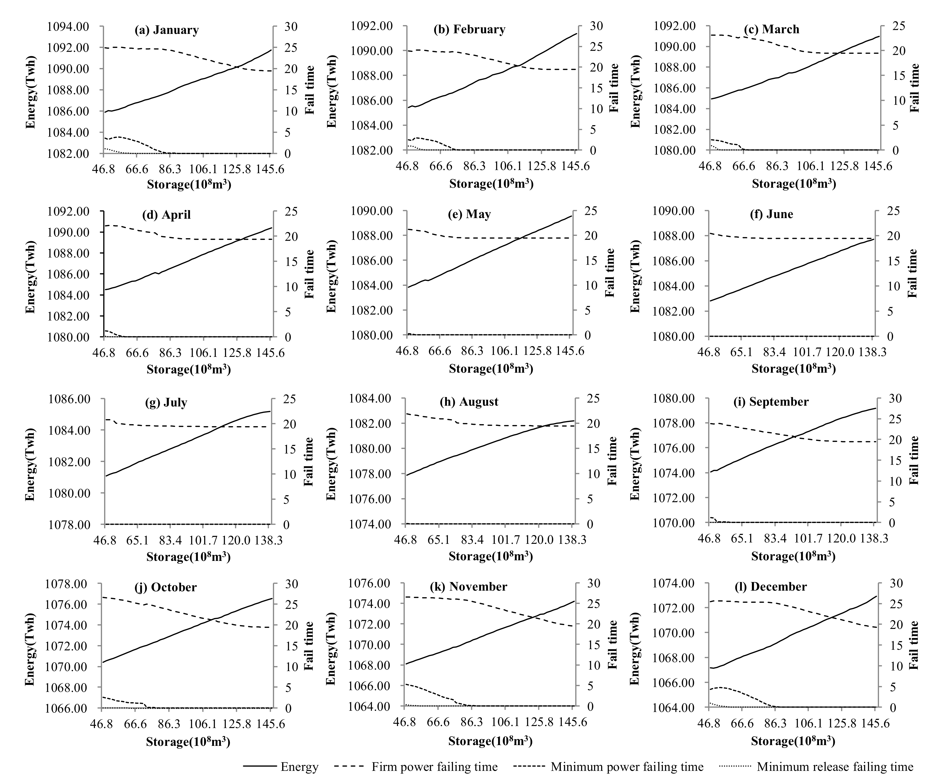
Figure 4 and Figure 5 show the future value functions of the energy and failing risks using ${\underset{\_}{p}}_1$, for time independent inflow MLDC-SDP and MLDC-SSDP. If the solutions converge for no more than five iterations in a year, 56 iterations are used to obtain the objective value curves for the whole simulated time horizon. The failing time and energy are the expected values over 56 years. It can be seen that in the dry season from November to March of the next year, the firm power failing risks are kept at a higher level with little change in the low storage area, and a fast reduction to lower levels at the middle storage area with an increase in storage. In the flood months of May to August, the risk decreases quickly with an increase in storage, even at low storage areas, and changes little at the high reservoir level area. In the area where the risk changes little with storage, the minimum failing time can be slightly reduced by operations, and operations in the dry season have a greater potential to reduce risk.

The initial reservoir level of the simulation is set near the upper bounds of January of the first year, so the simulation objective results should be close to the objective values corresponding to the upper bounds of January in Figure 4 and Figure 5, if the model exactly describes the problem. The simulation energy is 1083.6 TWh and 1086.5 TWh, and the value according to initial reservoir levels is about 1106.0 TWh and 1092.0 TWh for the MLDC-SDP and MLDC-SSDP models, respectively. For the monthly firm power failing time, the simulation values are 24 and 25 times, and the expected objective values for the initial reservoir level is about 3 and 20 times for the MLDC-SDP and MLDC-SSDP models, respectively. It can be seen that the objective functions of the models considering periodical inflow correlations are closer to the simulation results than the period inflow-independent MLDC-SDP. It is notable that even the simulation results are close to each other, and the computed expected values, especially the failing time values of the models, can be very different from each other. The failing time estimation of the independent inflow model apparently cannot reflect the real risks, as the reservoir has carry-over storage and most firm power failure is caused by continuous low inflow, which can be better formulated using models considering time correlations of inflow.

In the results of the single reservoir case study, both MLDC-SSDP and MLRC-SSDP obtain 100% reliabilities on $\underset{\_}{P}$ for both values of ${\underset{\_}{P}}_1$ and ${\underset{\_}{P}}_2$ (Table 2), indicating that the methods can reflect the constraint priority better than the other methods. Sometimes, the satisfaction of a higher-level constraint may cause low reliability on lower-level constraints. When the higher-level constraint is easily satisfied, the advantages of MLDC-SSDP and MLRC-SSDP may not be reflected by the simulation results. For example, when $\underset{\_}{p}={\underset{\_}{p}}_1$ is used, the reliabilities on fp using MLDC-SSDP and MLRC-SSDP are lower than the other two methods.

3.3. Cascaded Reservoir System Case Study

The model and method are then used for the whole cascaded system, taking the releases of the Xiaowan (numbered 1) and Nuozhadu (numbered 2) reservoirs as decision variables, and the reservoir levels of other reservoirs are set to be fixed in each month. The constraints of the reservoirs are set as four levels: $r_t^1\ge {\underset{\_}{r}}_1$, ${\underset{\_}{r}}_1$ = 470 m³s⁻¹ is the minimum outflow of Xiaowan reservoir; $r_t^2\ge {\underset{\_}{r}}_2$, ${\underset{\_}{r}}_2$ = 500 m³s⁻¹ is the minimum outflow of Nuozhadu reservoir; ${\displaystyle {\sum }_{m=1}^M{p}_m^t}\ge \underset{¯}{P}$, M is the reservoir number, $\underset{\_}{P}$ is the whole cascade minimum power; ${\displaystyle {\sum }_{m=1}^M{p}_m^t}\ge FP$, FP = 6800 MW is the whole cascade firm power.The constraints of reliabilities on whole cascade firm power, minimum whole cascade power, minimum release for Xiaowan and minimum release for Nuozhadu are set to be ${\gamma }_j=1$, j = 1, 2, 3, 4 in Equation (2), and the priorities of the constraints are reflected by the values of coefficients by setting ${\lambda }_1=1\times {10}^{10}$, ${\lambda }_2=1\times {10}^{20}$, and ${\lambda }_3={\lambda }_4=1\times {10}^{30}$.

In the MLDC-SDP, five local inflow intervals for each reservoir are used to obtain discretized joint probability distributions at each period. Local inflows to the Manwan and Dachaoshan reservoirs are supposed to be frequency synchronous with the Xiaowan reservoir inflows, and local inflows to Jinghong reservoir are supposed to be frequency synchronous with the Nuozhadu reservoir inflows.

For all of the models that can be concave, at a state, the optimal solution is found by searching multiple regions. The regions include possible local optimal regions found according to the coarse traversing of $51\times 51$ discretized decisions, and also include regions near the optimal solutions of the states that have been found around the current states. Converging after five times of yearly iteration, the solution time of MLDC-SDP and MLRC-SDP is over 130 h, and the solution time of MLDC-SSDP and MLRC-SSDP is over 300 h. The SSDP-based models take more time, as there are 56 samples to be computed in each state, while for the SDP-based models, there are only 25 discretized inflow combinations to compute.

Table 3. Computing results for the cascaded reservoirs.

Minimum Power Setting	Method	Energy (TWh)	Reliability on Firm Power (%)	Reliability on Minimum Power (%)
60% of firm power	MLDC-SDP	3841.2	96.6	100
	MLDC-SSDP	3841.3	99.1	100
	MLRC-SDP	3842.5	96.3	99.9
	MLRC-SSDP	3840.9	99.3	100
90% of firm power	MLDC-SDP	3822.0	33.6	98.5
	MLDC-SSDP	3822.3	37.4	100
	MLRC-SDP	3833.9	50.4	98.5
	MLRC-SSDP	3829.8	48.2	98.1

shows the computing results using a minimum power of $\underset{\_}{P}={\underset{\_}{P}}_1$ = 60%FP and $\underset{\_}{P}={\underset{\_}{P}}_2$ = 90%FP. When $\underset{\_}{P}={\underset{\_}{P}}_1$, the satisfying rates for $\underset{\_}{P}$ are almost the same using the four methods, and the SSDP-based models perform better than the SDP-based models for larger satisfying rates for higher-level constraints of $\underset{\_}{P}$, while there is no considerable difference between MLDC-based methods and RCDP-based methods. When $\underset{\_}{P}={\underset{\_}{P}}_2$, MLDC-SSDP performs best for the satisfying rates for $\underset{\_}{P}$ using MLDC-SSDP, which is larger than the other three methods by 1.5–1.9%.

Different from the single reservoir case, the energy generation is decreased using ${\underset{\_}{P}}_2$ compared to ${\underset{\_}{P}}_1$. This is because to satisfy ${\underset{\_}{P}}_2$, the dry season water release of large reservoirs can be more than to satisfy ${\underset{\_}{P}}_1$, causing lower reservoir levels and smaller flood season release. Thus, the inflow of lower stream reservoirs is increased in the dry season and decreased in the flood season, reducing the energy loss from spill.

Table 4. Energy generation using MLDC-SSDP.

Reservoir	Energy (TWh)
	$\underset{\_}{\mathit{p}}=60\mathit{\%}\mathit{F}\mathit{P}$	$\underset{\_}{\mathit{p}}=90\mathit{\%}\mathit{F}\mathit{P}$
Xiaowan	1071.9	1086.5
Manwan	451.8	444.9
Dachaoshan	420.7	412.7
Nuozhadu	1439.7	1439.0
Jinghong	457.1	450.8

shows the energy generation of the reservoirs using MLDC-SSDP for ${\underset{\_}{P}}_1$ and ${\underset{\_}{P}}_2$. It can be seen that the energy of the Xiaowan reservoir is still larger for ${\underset{\_}{P}}_1$ than ${\underset{\_}{P}}_2$, while the energy for the other reservoirs is less for ${\underset{\_}{P}}_1$ than ${\underset{\_}{P}}_2$.

MLDC-SSDP is the only method that obtains 100% reliabilities on $\underset{\_}{P}$ for all examples of single and cascaded reservoir operations (Table 2 and Table 3), indicating that the method can reflect the constraint priority better than the other methods.

4. Conclusions

The operation of hydropower reservoirs is to maximize economic benefit, subjected to constraints for social and noneconomic requirements. The constraints can generally be addressed using penalty terms or chance-constrained models. With the reinforcement of the demands of ecology, navigation, water supply, power compensation, etc., explicit priorities must be set for the constraints instead of being balanced using penalties, or be satisfied at a reliability. For the operation of hydropower systems with multiple constraints that can be sorted according to priorities, the RCDP-based models of MLRC-SDP and MLRC-SSDP and the explicit DC reasoning-based models of MLDC-SDP and MLDC-SSDP are proposed. A case study of the Lancang River reservoir system is presented, taking minimum release, minimum power, and firm power as constraints. The results show that the period correlations of inflows are important factors to reduce the chance of failure of the power constraints. For reservoirs with carry-over storage, the simulation results are good, the estimations for failing time may have quite large errors, and the estimations of the expected failing time need information on time correlation more than energy objectives. The MLDC-SSDP obtained better overall performance than the other methods, in that the constraint priorities were fully reflected and the reliabilities on higher-level constraint of minimum power are no less than the other methods, in all tested cases. Moreover, MLDC-SSDP performs greater reliability on firm power as the minimum power output constraint improves. The proposed model is suitable for hydropower reservoirs with strict social requirements or legal regulations.