
Economic Analysis of Heat Distribution Concepts for a Small Solar District Heating System


Abstract
:1. Introduction
1.1. Background
1.2. Previous Work
1.3. Aim and Scope
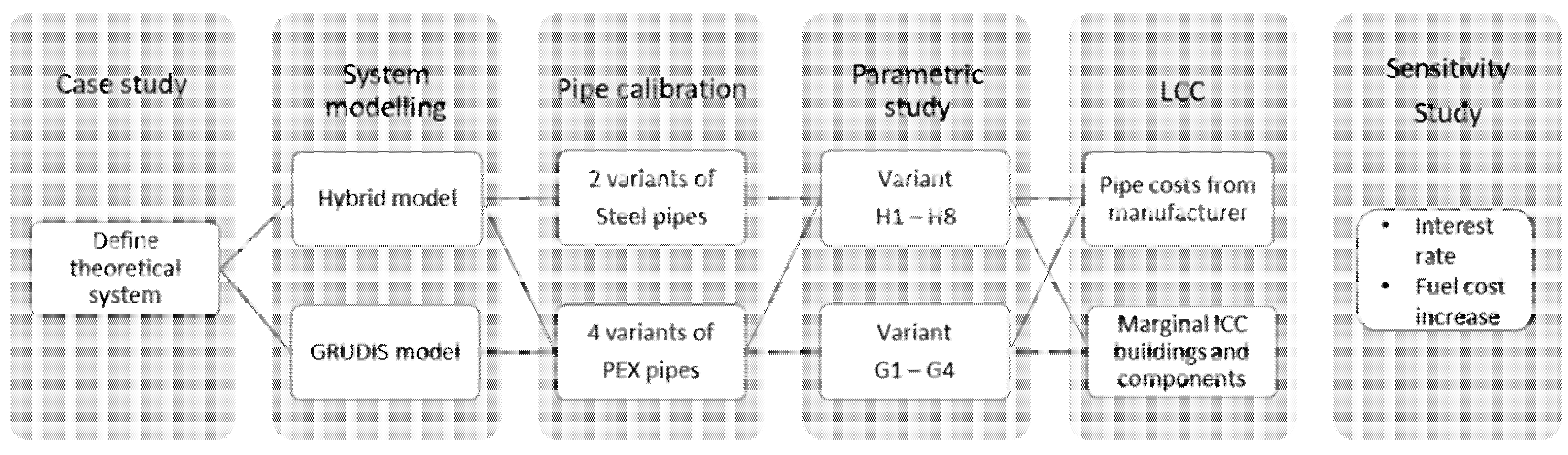
1.4. Overall Method
2. Case Study
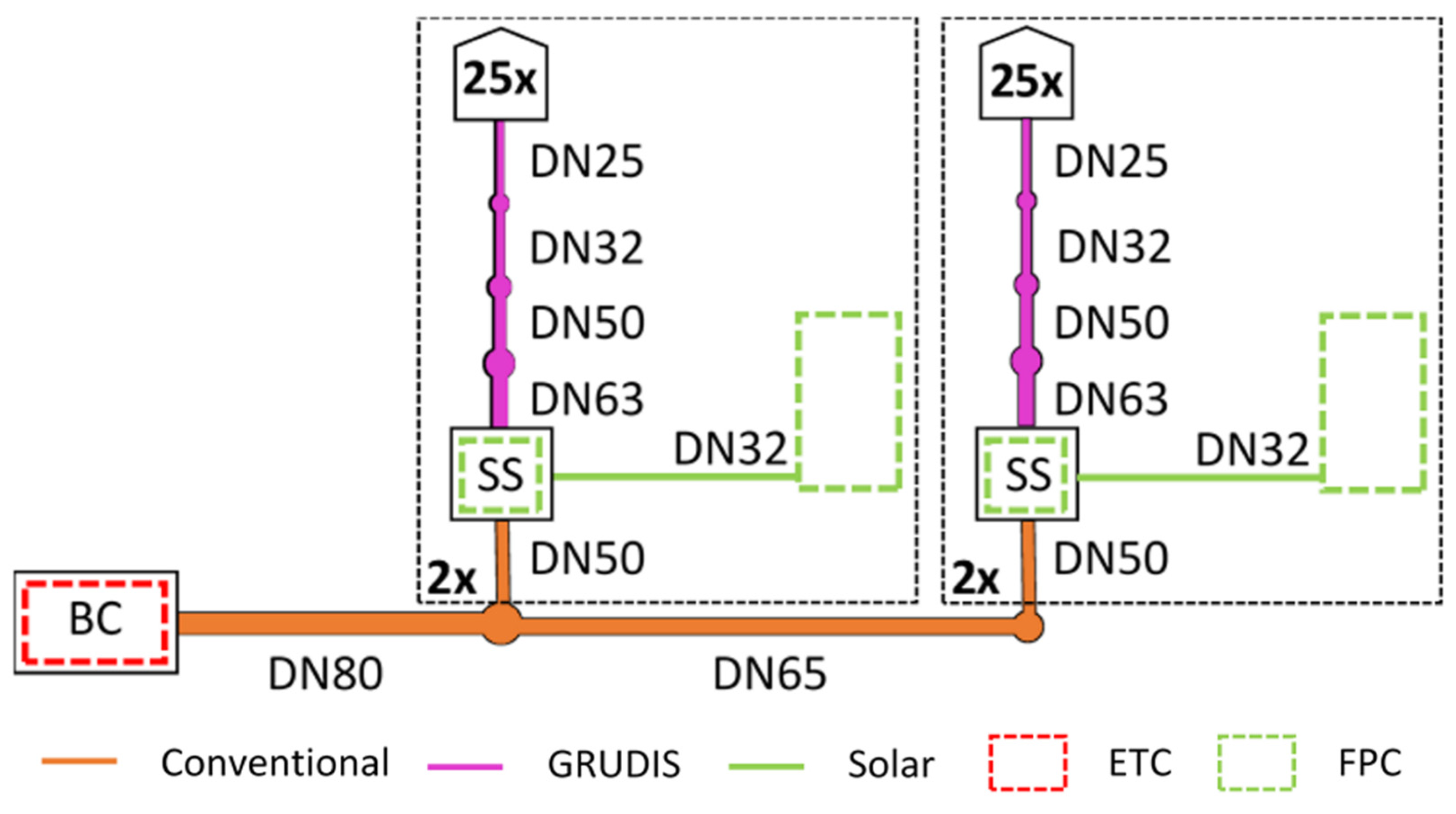
2.1. Solar District Heating System Layout
2.2. Heat Supply
2.3. Distribution Systems
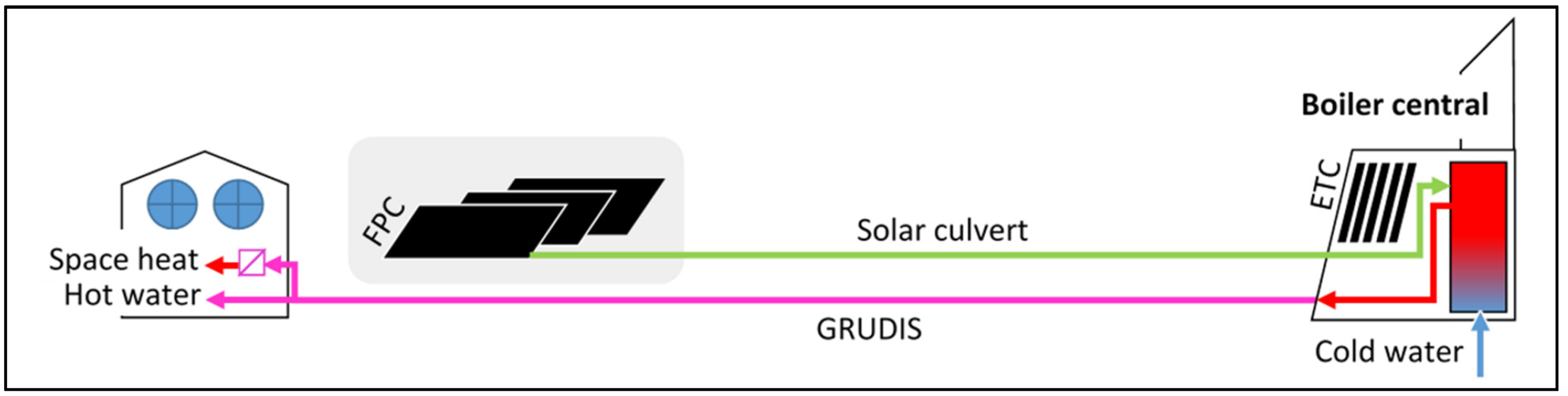
2.3.1. GRUDIS
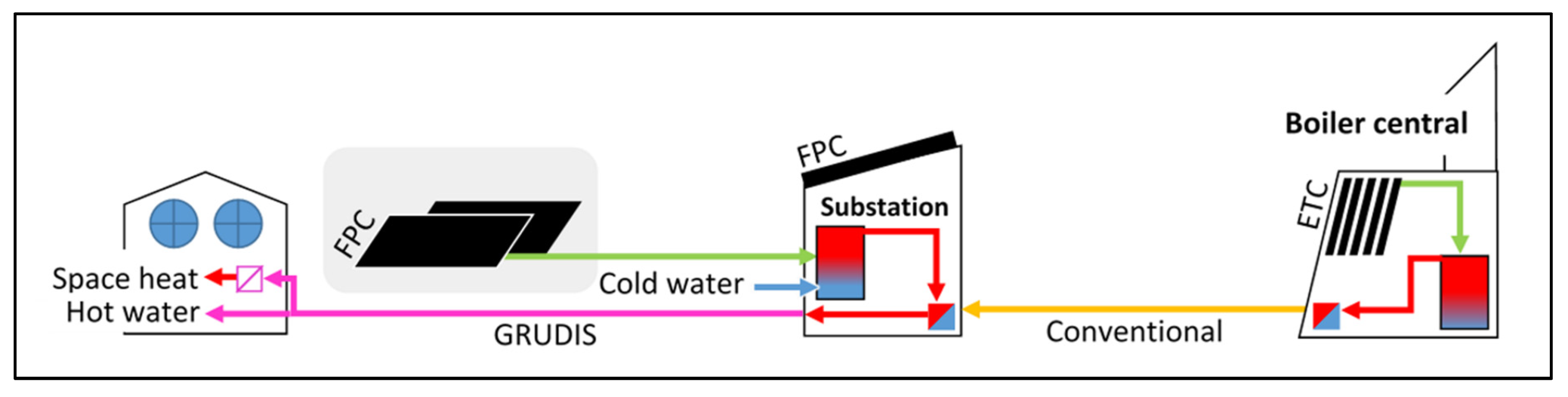
2.3.2. Hybrid Distribution Concept
2.4. Boundary Conditions and Heat Demand
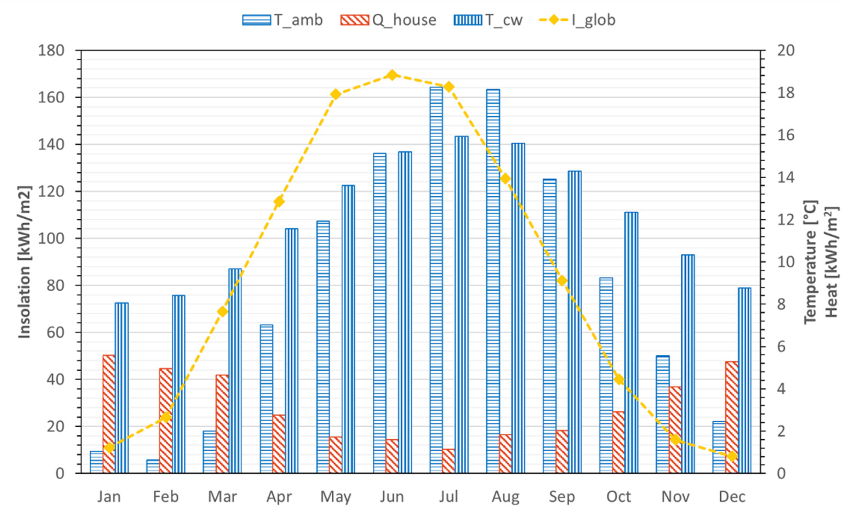
2.4.1. Climate Data and Heat Demand
2.4.2. DHW Profiles
3. Method
3.1. Modelling Approach for Deriving Energetic KPIs
- Building and house substation model (SH load × 25 = one housing area).
- Intermediate substation model (load × 2 = subsystem load) and ST system.
- Boiler central model.
3.1.1. Common Components for All System Models
3.1.2. Building and Space-Heating Model
3.1.3. Distribution Pipe Model
3.1.4. Reference Pipe Types and Combinations
3.1.5. Calibration of Pipe Losses
3.2. Parametric Study
3.3. Calculation of Life Cycle Cost
3.3.1. Summary of Economic Boundary Conditions
3.3.2. Initial Capital Costs (ICC)
3.3.3. Annual Operation and Maintenance Costs (A)
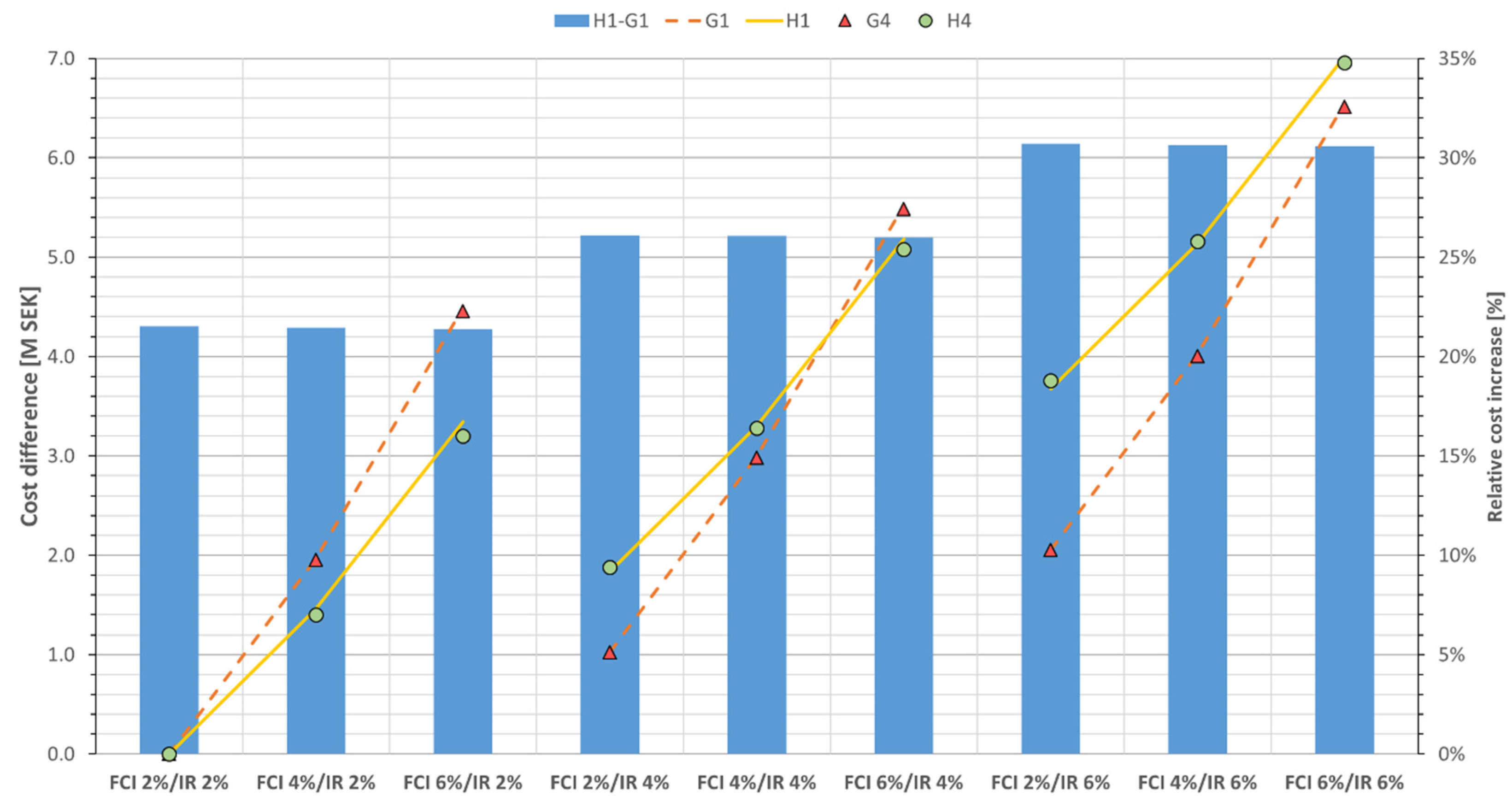
3.4. Cost Sensitivity Analysis
- Interest rate (IR): IR1, IR2, and IR3 correspond to p.a. 2%, 4%, and 6%, respectively.
- Boiler fuel cost increase (FCI): FCI1, FCI2 and FCI3 corresponding to p.a. increase of 2%, 4% and 6%, respectively.
- Economic lifetime: 20 years reference and 30 years extended.
3.5. Key Performance Indicators (KPI)
4. Results
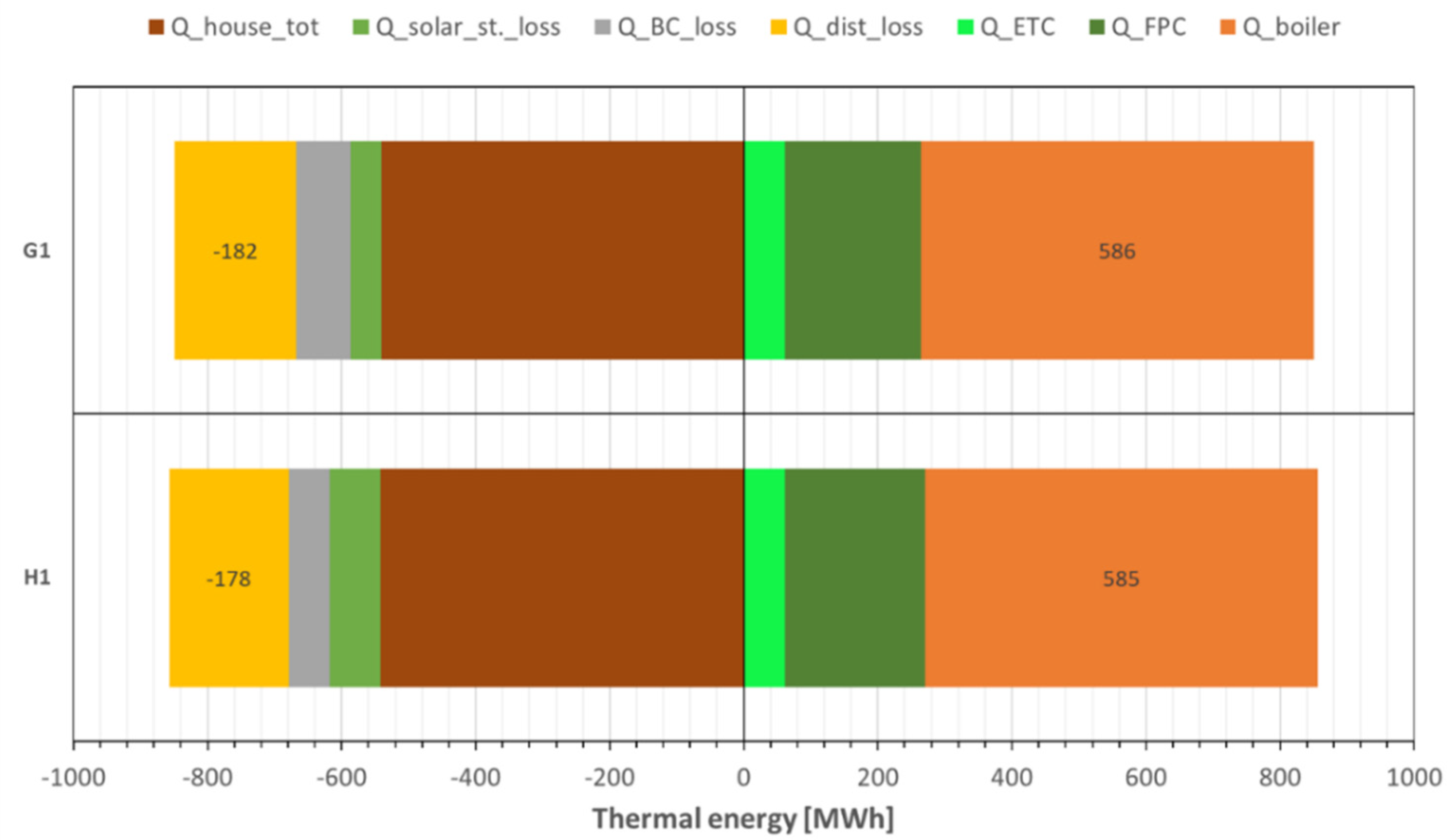
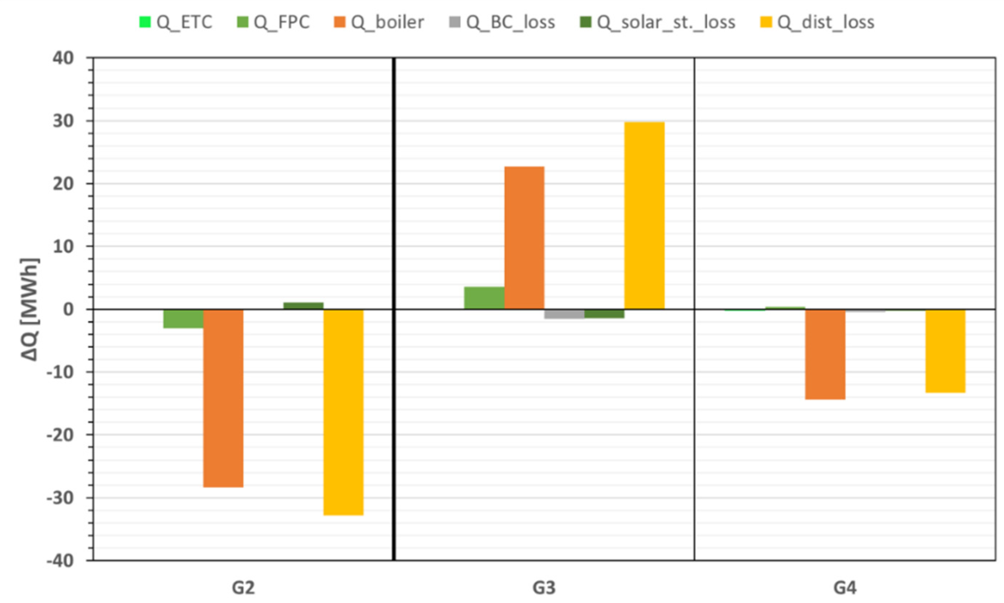
4.1. Energy Balance for Reference Pipes
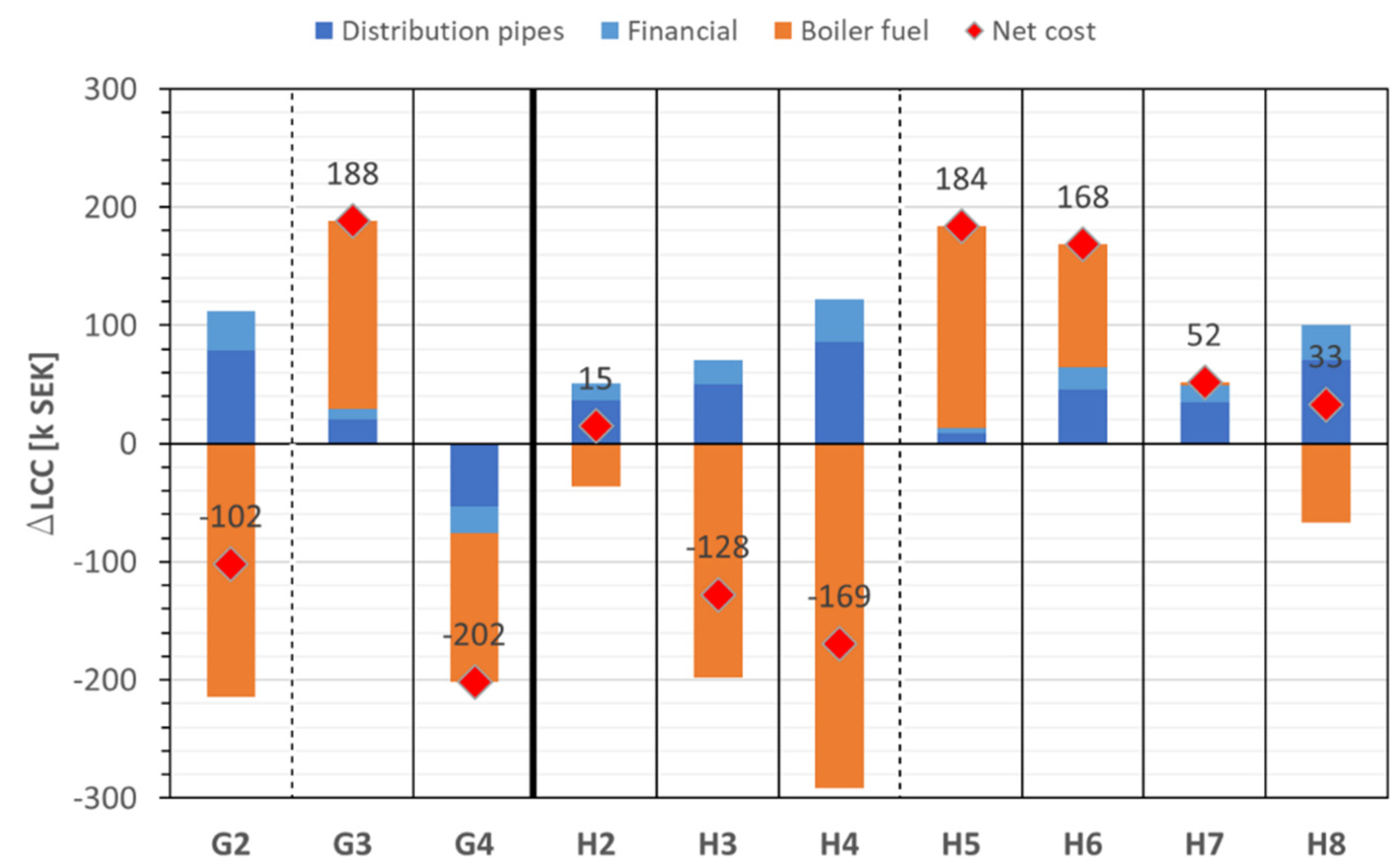
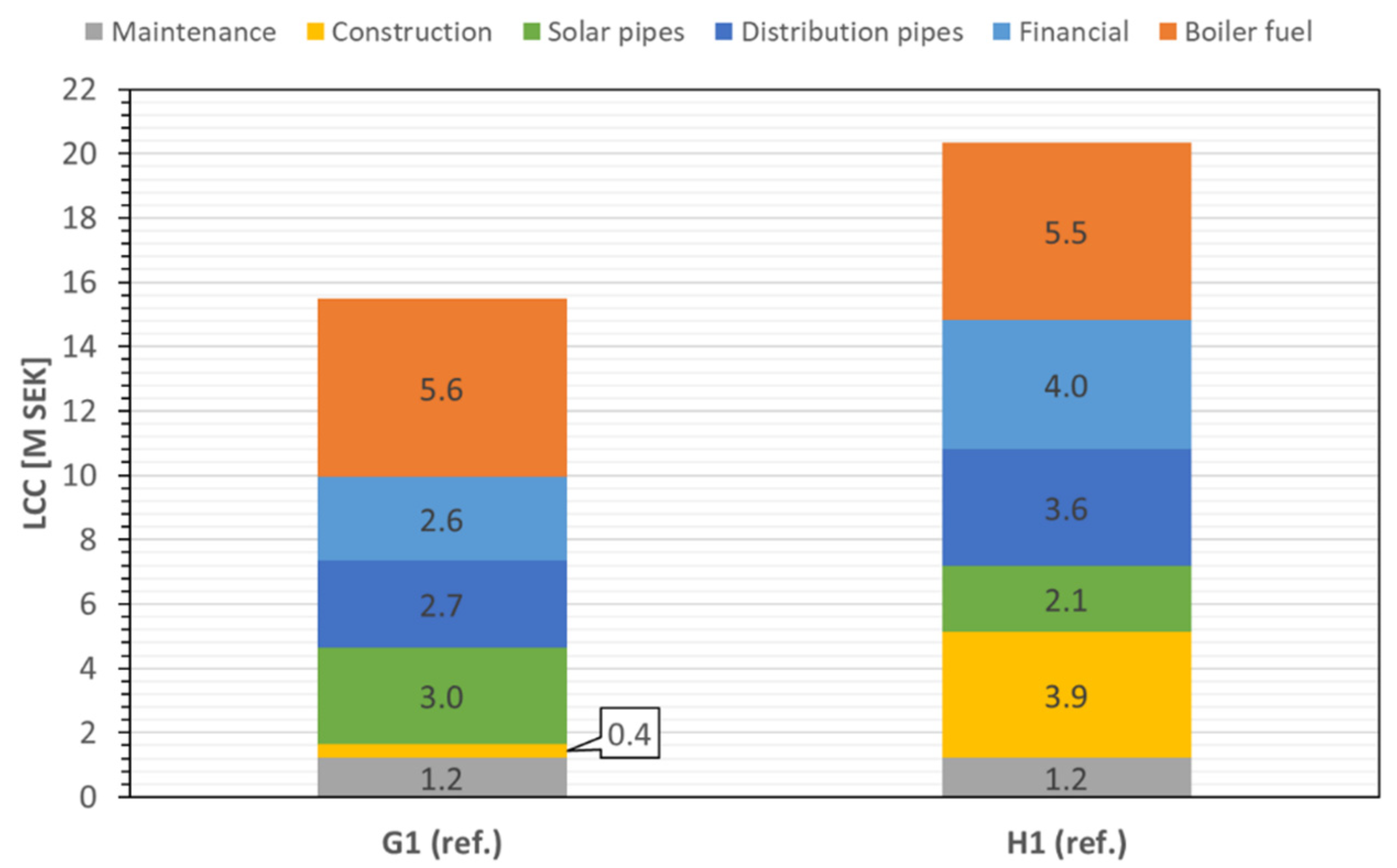
4.2. Life Cycle Cost
4.3. Parametric Study
4.3.1. Energy vs. Insulation Level
4.3.2. Costs vs. Change in Insulation Level
4.4. Sensitivity Analysis
5. Discussion
5.1. Modelling
5.1.1. Model Simplifications
- One housing area to represent two housing areas.
- One house model to represent all houses.
- Load connected to the supply at the end of the network.
5.1.2. Boiler Modulating Behaviour
5.2. Cost Calculations
5.2.1. Calculations from Price List vs. from Supplier
- Tenders from suppliers are without vendor margins (below market price).
- Possibility of tenders being undervalued (potential market strategy).
5.2.2. Cost Level in Calculation Software Wikells
5.2.3. Fuel Costs
6. Conclusions
- A hypothetical district heating system has been modeled in TRNSYS using two distribution concepts; a hybrid comprised of 3rd and 4th generation DH technology and GRUDIS, which may be considered 4th generation DH technology.
- A range of pipe insulation levels has been simulated for each concept, and the average boiler-supplied energy is similar for both the GRUDIS and Hybrid distribution concepts.
- Increase/decrease in heat losses due to change in insulation levels primarily affects the boiler supplied energy and, to a minor extent, solar contribution. The reduction in boiler supplied energy is at best 5% for the GRUDIS concept and 7% for the Hybrid concept.
- The lowest pipe network losses are found for a hybrid system variant using the highest available insulation level for both steel pipes and PEX pipes. The GRUDIS variant with the lowest pipe heat loss uses the PEX pipes with the highest insulation level.
- The LCC is highest for the hybrid concept, being 20.4 M SEK on average for all variants simulated, compared to 15.5 M SEK for all variants of the GRUDIS concept—a difference of the average of 24%.
- An annual increase in fuel cost of 2–6% has a negligible influence on differences in LCC between the hybrid and GRUDIS concept, whereas an interest rate of 2–6% has a significant impact on the differences due to the larger initial capital cost associated with the construction and consequently, financing of, the hybrid system.
- Simplifications made in the modeling approach appear to have an insignificant influence on the results, as these are based on inter-comparison between systems built on the same assumptions.
- The influence of the cost calculation method appears to have little to no effect on the difference in LCC between the distribution concepts, as different types of cost input for the calculation of pipe network costs give similar results.
7. Future Work
Author Contributions
Funding
Data Availability Statement
Acknowledgments
Conflicts of Interest
Nomenclature
| Abbreviations | |
| BC | Boiler Central |
| DH | District Heat(ing) |
| DHW | Domestic Hot Water |
| DN | Nominal Diameter |
| EPS | Extruded Polystyrene |
| EPSPEX | EPS encased PEX pipe(s) |
| ETC | Evacuated Tube Collector(s) |
| EUR | Euro |
| FCI | Fuel Cost Increase |
| FPC | Flat Plate Collector(s) |
| GRUDIS | Swedish acronym for “Gruppcentraldistributionssystem” |
| GM | Ground Mounted |
| G1–G4 | GRUDIS system variant 1 (reference) to 4 |
| H1–H8 | Hybrid system variant 1 (reference) to 8 |
| HVAC | Heating, Ventilation and Cooling |
| ICC | Initial Capital Cost(s) |
| IR | Interest Rate |
| KPI | Key Performance indicators |
| LCC | Life Cycle Cost |
| MA | Moving Average |
| MTR | Minimum turndown ratio; quotient minimum/maximum possible power output. |
| NPV | Net Present Value |
| O&M | Operation & Maintenance |
| PI-PEX | Pre-Insulated PEX pipe(s) |
| PEX | Cross-linked Polyethylene |
| SDH | Solar district heating |
| SEK | Swedish Krone(s) |
| SF | Solar Fraction |
| SH | Space Heating |
| SS | Substation |
| SS-EN | Swedish Standard - Engineering Norm |
| ST | Solar Thermal |
| TMY | Typical Meteorological Year |
| Symbols | |
| A | Annual O&M cost |
| R | Re-investment cost |
| Res | Residual value |
| L | Length [m] |
| M | Million; 106 |
| Q | Heat energy [J/kWh] |
| ∆Q | Difference in heat energy |
| Heat loss [W] | |
| Specific heat loss [W/m] | |
| η | Efficiency |
| K | Empirical constant for use in calculation of boiler efficiency |
| β | Boiler load factor |
| t | Time [h] |
References
- Lund, H.; Werner, S.; Wiltshire, R.; Svendsen, S.; Thorsen, J.E.; Hvelplund, F.; Mathiesen, B.V. 4th Generation District Heating (4GDH): Integrating smart thermal grids into future sustainable energy systems. Energy 2014, 68, 1–11. [Google Scholar] [CrossRef]
- Mathiesen, B.V.; Bertelsen, N.; Schneider, N.C.A.; García, L.S.; Paardekooper, S.; Thellufsen, J.Z.; Djørup, S.R. Towards a Decarbonised Heating and Cooling Sector in Europe Unlocking the Potential of Energy Efficiency and District Energy; Aalborg Universitet: Aalborg, Denmark, 2019. [Google Scholar]
- Weiss, W.; Spörk-Dür, M. Solar Heat Worldwide—Global Market Developments and Trends in 2020; AEE Intec; IEA SHC: Gleisdorf, Austria, 2021. [Google Scholar]
- Eurostat. Eurostat: Just over 20% of Energy Used for Heating and Cooling is Renewable. 2019. Available online: https://ec.europa.eu/eurostat/en/web/products-eurostat-news/-/ddn-20201229-1 (accessed on 29 April 2022).
- REN21. Renewables 2020 Global Status Report; REN21 Secretariat: Paris, France, 2020. [Google Scholar]
- REN2021. Renewables in Cities 2021 Global Status Report; REN21 Secretariat: Paris, France, 2021. [Google Scholar]
- Averfalk, H.; Werner, S. Essential improvements in future district heating systems. Energy Procedia 2017, 116, 217–225. [Google Scholar] [CrossRef]
- Werner, S. Fourth Generation of District Heating Technology. Fininish District Heating Days 2017. 2017. Available online: https://www.4dh.eu/resources/publications (accessed on 25 November 2020).
- Mauthner, F.; Herkel, S. IEA SHC Task 52: Solar Heat and Energy Economics in Urban Environments—Technical Report Subtask C—Part C1; IEA SHC: Cedar, MI, USA, 2016. [Google Scholar]
- Mauthner, F.; Joly, M. IEA SHC Task 52: Solar Heat and Energy Economics in Urban Environments—Technical Report Subtask B/C—Part B3/C2; IEA SHC: Cedar, MI, USA, 2017. [Google Scholar]
- Andersen, M. Solar District Heating for Low Energy Residential Areas; Chalmers University of Technology: Gothenburg, Sweden, 2019. [Google Scholar]
- Andersen, M.; Bales, C.; Dalenbäck, J. Heat Distribution Concepts for small Solar District Heating Systems—Techno-economic study for low line Heat densities. Energy Convers. Manag. X 2022, 15, 100243. [Google Scholar] [CrossRef]
- Zinko, H. GRUDIS-Tekniken för Värmegles Fjärrvärme; Rapport Värmegles 2004:10; Svensk Fjärrvärme AB: Stockholm, Sweden, 2004; ISSN 1401-9264. [Google Scholar]
- Zinko, H.; Bøhm, B.; Kristjansson, H.; Ottoson, U.; Räma, M.; Sipilä, K. IEA R&D Programme on ‘District Heating and Cooling, Including the Integration of CHP’; Annex VIII, District Heating Distribution in Areas with Low Heat Demand Density; IEA DHC: Frankfurt, Germany, 2008. [Google Scholar]
- Persson, C.; Fröling, M.; Svanström, M. Life Cycle Assessment of the District Heat Distribution System—Part 3: Use Phase and Overall Discussion (10 pp). Int. J. Life Cycle Assess. 2006, 11, 437–446. [Google Scholar] [CrossRef]
- Cool, D.H. Cool DH—Cool District Heating; Innovations; Cool DH, HOR2020. 2022. Available online: http://www.cooldh.eu/demo-sites-and-innovations-in-cool-dh/innovations/ (accessed on 3 March 2022).
- Rosa, A.D.; Li, H.; Svendsen, S.; Werner, S.; Persson, U.; Rühling, K.; Felsmann, C.; Crane, M.; Burzynski, R.; Bevilacqua, C. Annex X Final report: Toward 4th Generation District Heating: Experience and Potential of Low-Temperature District Heating. IEA Annex X 2014, 205, 107751645. [Google Scholar]
- Olsson, H.; Rosander, A. Evaluation of the Solar-Assisted Block Heating System in a Passive House Residential Area. Master’ s Thesis, Chalmers University of Technology, Gothenburg, Sweden, 2014. [Google Scholar]
- Nielsen, C.; Haegermark, M.; Dalenbäck, J.O. Analysis of a Novel Solar District Heating System. In Proceedings of the ISES and IEA SHC International Conference on Solar Energy for Buildings and Industry, Kassel, Germany, 25–29 September 2022; pp. 16–19. Available online: http://urn.kb.se/resolve?urn=urn:nbn:se:du-15517 (accessed on 29 April 2022).
- Andersen, M.; Bales, C.; Dalenbäck, J. Techno-economic Analysis of Solar Options for a Block Heating System. In Proceedings of the Eurosun 2016 Conference Proceedings, Palma de Mallorca, Spain, 11–14 October 2016. [Google Scholar]
- Wallentun, H.; Zinko, H. Medieror av Plast i Fjärrvärme System, FOU 1996:8 (Swedish); Swedish District Heating Association: Stockholm, Sweden, 1996. [Google Scholar]
- Gudmundson, T. EPSPEX-Kulvert: Utveckling, Utförande Och Uppföljning, FOU 2003:96; Swedish District Heating Association: Stockholm, Sweden, 2003. [Google Scholar]
- Dahm, J. Small District Heating Systems; Chalmers Tekn. Högskola: Gothenburg, Sweden, 1999. [Google Scholar]
- SEL; CSTB; TRNSOLAR; TESS. TRNSYS 17, a Transient System Simulation Program—Volume 1, Getting Started; University of Wisconsin: Madison, WI, USA, 2014; Volume 1, Available online: http://www.trnsys.com/ (accessed on 20 May 2022).
- Amnis Systemutveckling, Wikells Sektionsdata. 2021. Available online: https://wikells.se/ (accessed on 29 April 2022).
- Andersen, M. Data for Article: ‘Economic Analysis of Heat Distribution Concepts for a small Solar District Heating System’; Mendeley Data, V1; Elsevier: Amsterdam, The Netherlands, 2022. [Google Scholar] [CrossRef]
- Fahlén, E.; Olsson, H.; Sandberg, M.; Löfås, P.; Kilersjö, C.; Christensson, N.; Jessen, P.A. Vallda Heberg—Sveriges Största Passivhusområde Med Förnybar Energi; Lågan: Gothenburg, Sweden, 2014. [Google Scholar]
- Sotnikov, A.; Nielsen, C.K.; Bales, C.; Dalenbäck, J.O.; Andersen, M.; Psimopoulos, E. Simulations of a Solar-Assisted Block Heating System. In Proceedings of the ISES Solar World Congress 2017—IEA SHC International Conference on Solar Heating and Cooling for Buildings and Industry, Abu Dhabi, UAE, 29 October—2 November 2017; Volume 1, pp. 373–383. [Google Scholar] [CrossRef]
- Meteotest, v. 7.3.4. 2020. Available online: https://meteonorm.com/en/ (accessed on 29 April 2022).
- Jordan, U.; Vajen, K. DHWcalc—Tool for the Generation of Domestic Hot Water (DHW) Profiles on a Statistical Basis; Universität Kassel: Kassel, Germany, 2017; Volume 2, p. 22. [Google Scholar]
- TRNSYS. TRNSYS 17, a Transient System Simulation Program—Volume 4 Mathematical Reference; Solar Energy Laboratory, University of Wisconsin-Madison: Madison, WI, USA, 2009. [Google Scholar]
- TESS. TESS Component Libraries—General Descriptions; Thermal Energy System Specialists, LLC: Madison, WI, USA, 2021; p. 79. Available online: https://www.trnsys.com/tess-libraries/ (accessed on 29 April 2022).
- Drück, H. Transsolar: Type 340—MULTIPORT Store Model for TRNSYS. 2006. Available online: https://www.trnsys.de/static/788c19e80e1b4e690b35e44b05c8b164/ts_type_340_de.pdf (accessed on 17 March 2021).
- Gustafsson, M.S.; Myhren, J.A.; Dotzauer, E. Life Cycle Cost of Heat Supply to Areas with Detached Houses—A Comparison of District Heating and Heat Pumps from an Energy System Perspective. Energies 2018, 11, 3266. [Google Scholar] [CrossRef] [Green Version]
- Elgocell, A.B.; Klingheim, M. Personal communication, 2019.
- Sveriges Riksbank. riksbank.se; Current Inflation Rate. 2021. Available online: https://www.riksbank.se/en-gb/monetary-policy/the-inflation-target/current-inflation-rate/ (accessed on 22 June 2021).
- Lejenstrand, A. Welcome to Swedenergy—Energiföretagen Sverige. 2021. Available online: https://www.energiforetagen.se/in-english/ (accessed on 23 June 2021).
- Andersson, I.; Hultmark, A.B. Andersson & Hultmark. 2021. Available online: http://aohab.se/ (accessed on 14 April 2021).
- SCB. Electricity Supply, District Heating and Supply of Natural Gas 2019, Final Statistics; Swedish Energy Authority: Eskilstuna, Sweden, 2020. [Google Scholar]
- Sätila Bygg. Sätila Bygg, satilabygg.se. 2019. Available online: https://satilabygg.se/ (accessed on 22 June 2021).
- Carlon, E.; Schwarz, M.; Golicza, L.; Verma, V.K.; Prada, A.; Baratieri, M.; Haslinger, W.; Schmidl, C. Efficiency and operational behaviour of small-scale pellet boilers installed in residential buildings. Appl. Energy 2015, 155, 854–865. [Google Scholar] [CrossRef]
- Statens Energimyndighet. Scenarier över Sveriges Energisystem 2020 (Swedish); ER 2021:6; Statens Energimyndighet: Eskilstuna, Sweden, 2021; ISSN 1403-1892. [Google Scholar]


| Parameters | Hybrid | GRUDIS |
|---|---|---|
| Boiler | 300 kW | |
| ETC (tilt/azimuth) | 108 m2 (70°/0°) | |
| FPC (tilt/azimuth) | 177 m2 (SS) + 442 m2 (GM) 19°/25° (SS), 30°/20° (GM) | 619 m2 (GM) (30°/20°) |
| Storage tank | 15 m3 (BC) + (15 × 4) m3 (SS) | 15 m3 (BC) + 60 m3 (BC) |
| Component | GRUDIS Figure 2a/Figure 3 | Hybrid Figure 2b/Figure 4 |
|---|---|---|
| Boiler central | Storage for all collectors, DHW preparation | Storage for centralized collectors |
| Intermediate substation | N/A | Storage for distributed collectors, DHW preparation |
| House substation | SH only | SH only |
| Network pipes & design operating temperatures | Primary: PEX 60/50 °C | Primary: Steel 75/50 °C |
| Secondary: PEX 60/50 °C | ||
| Collectors | Centralized: ETC (BC) | Centralized: ETC (BC) |
| Distributed: FPC (BC) | Distributed: FPC (SS) |
| Name | Component Type | Main Parameters | Descriptions |
|---|---|---|---|
| Weather data | Type 15 | Kungsbacka, Sweden (57.5° N, 12.0° E), TMY | Data from Meteonorm 7 (v.7.3.4) |
| Boiler | Type 659 (TESS) [32] | 300 kW | Wood-pellet boiler |
| ETC | Type 538 (TESS) | 108 m2 | Fluid: water. Tilt 70, azimuth 0 |
| FPC | Type 832v501 | 620 m2; allocation varies according to concept (see Table 1) | Fluid: 40% propylene glycol/water. Int. substation: Tilt 19, azimuth 25 Ground-mounted array: Tilt 30, azimuth 20 |
| Tank(s) | Type 340 [33] | 15 m3/60 m3 | Diurnal storage; volume depends on system |
| Pump(s) | Type 3 | Max flow rate; Varied parameter values | Variable control signal, power consumption, and dissipation to fluid stream ignored. |
| House | Type 56 | Base area 70 m2, two zones, internal gains. | Internal gains: 400 W passive + 70% of electricity consumption [27]. |
| Heat recovery | Type 667 (TESS) | Rated power: 186.4 W, Effectiveness: 0.8. | Same effectiveness for both sensible and latent. |
| Water-air HEX | Type 670 (TESS) | Fluid: Propylene glycol. Effectiveness: 0.8. | Set point 19.5 °C for control of flow to component. |
| Twin-pipe(s) | Type 951(TESS) | Varied parameters for each pipe size and type. | Distribution network pipe for conventional and GRUDIS |
| Single pipe(s) | Type 952 (TESS) | Insulation thickness, heat transfer coefficient. | Distribution network pipe for GRUDIS. |
| Single pipe(s) | Type 709 (TESS) | Varied parameters according to pipe size | Connection pipes for solar collectors and internal supply pipes in BC and intermediate substations. |
| DHW load(s) | Type 9 | Flow rate | Generated DHW profiles, 1 profile per 50 houses. |
| Variant | G1 (ref) | H1 (ref) | |
|---|---|---|---|
| Primary | Pipe type | PI-PEX (M2) | Steel (M1) |
| Ins. class | Standard | Series 1 | |
| Secondary | Pipe type | NA | PI-PEX (M2) |
| Ins. class | NA | Standard |
| Pipe Type | Tsupply [°C] | Treturn [°C] | Tground [°C] | Soil cover [m] | λsoil [W/m K] | λpipe [W/m K] | λins [10−2 W/m K] |
|---|---|---|---|---|---|---|---|
| Steel (M1) | 80.0 | 40.0 | 10.0 | 0.8 | 1.00 | 50.00 | 2.30 |
| PI-PEX (M2) | 0.38 | 1.99 | |||||
| PI-PEX (M1) | 2.20 | ||||||
| EPSPEX (M3) | 70.0 | 40.0 | 6.0 | 0.6 | 3.40 | ||
| Copper (M1) | 85.0 | 45.0 | 10.0 | 0.8 | 365.00 | 2.20 |
| Variant | H2 | H3 | H4 | H5 | H6 | H7 | H7 | |
|---|---|---|---|---|---|---|---|---|
| Primary | Pipe type | Steel (M1) | Steel (M1) | Steel (M1) | Steel (M1) | Steel (M1) | Steel (M1) | Steel (M1) |
| Ins. class | Series 2 | Series 1 | Series 2 | Series 1 | Series 2 | Series 1 | Series 2 | |
| Secondary | Pipe type | PI-PEX (M2) | PI-PEX (M2) | PI-PEX (M2) | PI-PEX (M1) | PI-PEX (M1) | EPSPEX (M3) | EPSPEX (M3) |
| Ins. class | Standard | Plus | Plus | Mixed | Mixed | NA 1 | NA 1 |
| Variant | G2 | G3 | G4 |
|---|---|---|---|
| Pipe type | PI-PEX (M2) | PI-PEX (M1) | EPSPEX (M3) |
| Ins. class | Plus | Mixed | NA1 |
| Cost Type | GRUDIS | Hybrid | Comment |
|---|---|---|---|
| Construction (ICC) | Larger boiler central; additional building costs apply. | Four intermediate substations; categorized into building, HVAC, and electric costs. | Differences in HVAC components and building material amount. |
| Pipe network (ICC) | PEX pipes for main and branch pipes. Installation costs 561 SEK/m [35,36]. | Steel pipes for main and branch pipes. Installation costs according to [37]. | Differences in pipe material and installation costs. |
| Financial (ICC) | Economic lifetime 20 years. 4% capital interest p.a. | Economic lifetime 20 years. 4% capital interest p.a. | Higher ICC gives higher capital interest costs. |
| Maintenance (A) | 50,000 SEK p.a. [38]. Inflation adjusted 2% p.a. | 50,000 SEK p.a [38]. Inflation adjusted 2% p.a. | Boiler inspection, cleaning, and repair. |
| Boiler fuel (A) | Boiler efficiency according to Equation (3). Solar collector degradation 0.5% p.a. Fuel cost 305 SEK/MWh [39]. | Boiler efficiency according to Equation (3). Solar collector degradation 0.5% p.a. Fuel cost 305 SEK/MWh [39]. | Solar collector degradation leads to an increase in boiler fuel use. |
| Qhouse tot | Total house (SH + DHW) energy demand in the DH network. |
| Qsolar st. loss | Losses from FPC solar storage plus internal connection pipes. |
| QBC loss | Losses from storage for ETC solar and boiler plus internal connection pipes. |
| Qdist loss | Losses from ground buried pipes. |
| QETC | Stored solar energy from evacuated tube collectors. |
| QFPC | Stored solar energy from flat plate collectors. |
| Qboiler | Energy supplied from the boiler to flow stream, excluding losses. |
| LCC | Life cycle cost |
| Variant | H4 | H3 | G2 | G4 | H8 | H2 | H7 | H1 | G1 | H6 | H5 | G3 |
|---|---|---|---|---|---|---|---|---|---|---|---|---|
| [kW] | −15.9 | −16.8 | −17.0 | −19.3 | −19.4 | −19.4 | −20.3 | −20.3 | −20.8 | −21.4 | −22.4 | −24.2 |
| [W/m] | −6.1 | −6.5 | −6.0 | −7.5 | −7.5 | −7.5 | −7.9 | −7.9 | −7.3 | −8.3 | −8.7 | −8.5 |
| Net. L [m] | 2580 | 2580 | 2840 | 2580 | 2580 | 2580 | 2580 | 2580 | 2840 | 2580 | 2580 | 2840 |
Publisher’s Note: MDPI stays neutral with regard to jurisdictional claims in published maps and institutional affiliations. |
© 2022 by the authors. Licensee MDPI, Basel, Switzerland. This article is an open access article distributed under the terms and conditions of the Creative Commons Attribution (CC BY) license (https://creativecommons.org/licenses/by/4.0/).
Share and Cite
Andersen, M.; Bales, C.; Dalenbäck, J.-O. Economic Analysis of Heat Distribution Concepts for a Small Solar District Heating System. Energies 2022, 15, 4737. https://doi.org/10.3390/en15134737
Andersen M, Bales C, Dalenbäck J-O. Economic Analysis of Heat Distribution Concepts for a Small Solar District Heating System. Energies. 2022; 15(13):4737. https://doi.org/10.3390/en15134737
Chicago/Turabian StyleAndersen, Martin, Chris Bales, and Jan-Olof Dalenbäck. 2022. "Economic Analysis of Heat Distribution Concepts for a Small Solar District Heating System" Energies 15, no. 13: 4737. https://doi.org/10.3390/en15134737
APA StyleAndersen, M., Bales, C., & Dalenbäck, J.-O. (2022). Economic Analysis of Heat Distribution Concepts for a Small Solar District Heating System. Energies, 15(13), 4737. https://doi.org/10.3390/en15134737