Predicting Mining Areas Deformations under the Condition of High Strength and Depth of Cover

Abstract

This paper presents an analysis of mining area deformations in the rock mass consisting of high depth and strength strata deposited in the cover. The analysis of land surveying results enabled the identification of the parameters required to predict subsidence, which differed from the typical parameters for the Upper Silesian Coal Basin. The parameters of the Budryk–Knothe theory were determined based on the results of geodetic measurements. The calculations of the final state of deformations for planned mining were made using the average and characteristics for the study area parameter values. Based on experience, it is known that the range of subsidence trough depends on the mechanical properties of the rock mass. This study shows that the presence of high-strength rocks also reduces the value of the coefficient of roof control. Subsequently, calculations were made by a computer simulation of longwall mining to determine the course of indices of deformation over time. The calculations were conducted twice: on the assumption that the impact was immediate and on the assumption of the parameter values typical for the basin, and formula expressing the course of subsidence over time with the parameter values based on the measurement results. The obtained distributions of deformation indicators were diametrically opposed to each other. The results of the calculations with the parameter values appropriate for the region indicate that it is possible to carry out a planned mining operation without creating a risk to objects on the surface.

1. Introduction

In Europe, hard coal extraction is being constantly reduced. For instance, in Poland the extraction of this raw material decreased from approximately 200 million Mg in the 1970s to approximately 70 million Mg currently [1]. Hard coal mining in Russia or China remains more or less at a stable level, or at least it is not being reduced so drastically [2] and amounts to approximately 3.5 billion Mg. Coal and metal ore deposits are deposited in many basins under highly urbanized areas [3,4,5]. This requires that mining be conducted in a way that minimizes its impact on the surface, building structures and the city infrastructure above it [2,6]. Having an appropriate mathematical formula to predict post-mining surface deformations determines the effective prevention of mining and construction damage. Therefore, we observe the development of theories that aim to predict the mining impacts on the rock mass and the surface. Among them, the following groups can be distinguished [4,7]:

• Solutions based on adopted axioms, which may be of empirical origin. This group consists of the solutions and the method developed in the United Kingdom by the National Coal Board–NCB, [5]. This group also contains the so-called geometrical-integral theories [8,9,10,11,12];
• Based on models of continuous media [13];
• Based on the stochastic medium theory [14]. In addition, the theory of cellular automata model is also applicable [15];
• Intermediate solutions–using models of the continuous medium and empirical axioms [16];
• Numerical methods that are gaining popularity due to the development of digital technology [17,18,19,20]. FLAC3D software is the most frequently used. Based on the software-based calculations, Gang and Yang [3] determined a safe distance from a mining boundary to an urbanized area, which allowed extracting 1.5 million Mg of coal and avoiding damage to surface structures. It should be noted that mining was conducted at a shallow depth, which made the preparation of the data relatively easy. To a great extent, the course of the deformation process undoubtedly depends on natural and geological conditions [4]. The geological structure of the rock mass especially has an impact on the extent of deformations or the kinetics of the process. This makes it necessary to have a good understanding of the parameter values used for predictions. In these cases, using numerical methods is very helpful; however, this also has certain limitations, because the parameters of the rock strength change during extraction. Capturing these changes in a model is both difficult and time-consuming. For instance, in the work of Zhu et al. [21], the analyses were conducted to determine the impact of the depth of loose overburden on the course of deformations using FLAC3D software.

It can be concluded that although numerical methods give great opportunities to conduct comprehensive analyses, they also require a good knowledge of a series of mechanical parameters of multiple strata. Moreover, in cases of intensive mining (many workings) at great depth, the preparation of data for calculations is very laborious. This results in the widespread application of the theories from group 1 in practice. They are used in the mining industry in Poland [4,7,8], Germany [5], the United States [22,23].

In addition, predictions should also take into account the time variable [8,10,11].

One should also consider the impact of geological and mining conditions on the parameter values needed for calculations. The structure of the rock mass and its properties have a particular impact here. When using average parameter values for a given area for calculations, the obtained results might differ significantly from the actual state. In this way, the analyses of the impact of mining on built structures will be heavily error-burdened, which has a significant impact on the safety of built structures users and the structures themselves. This article is devoted to these issues.

2. Materials and Methods

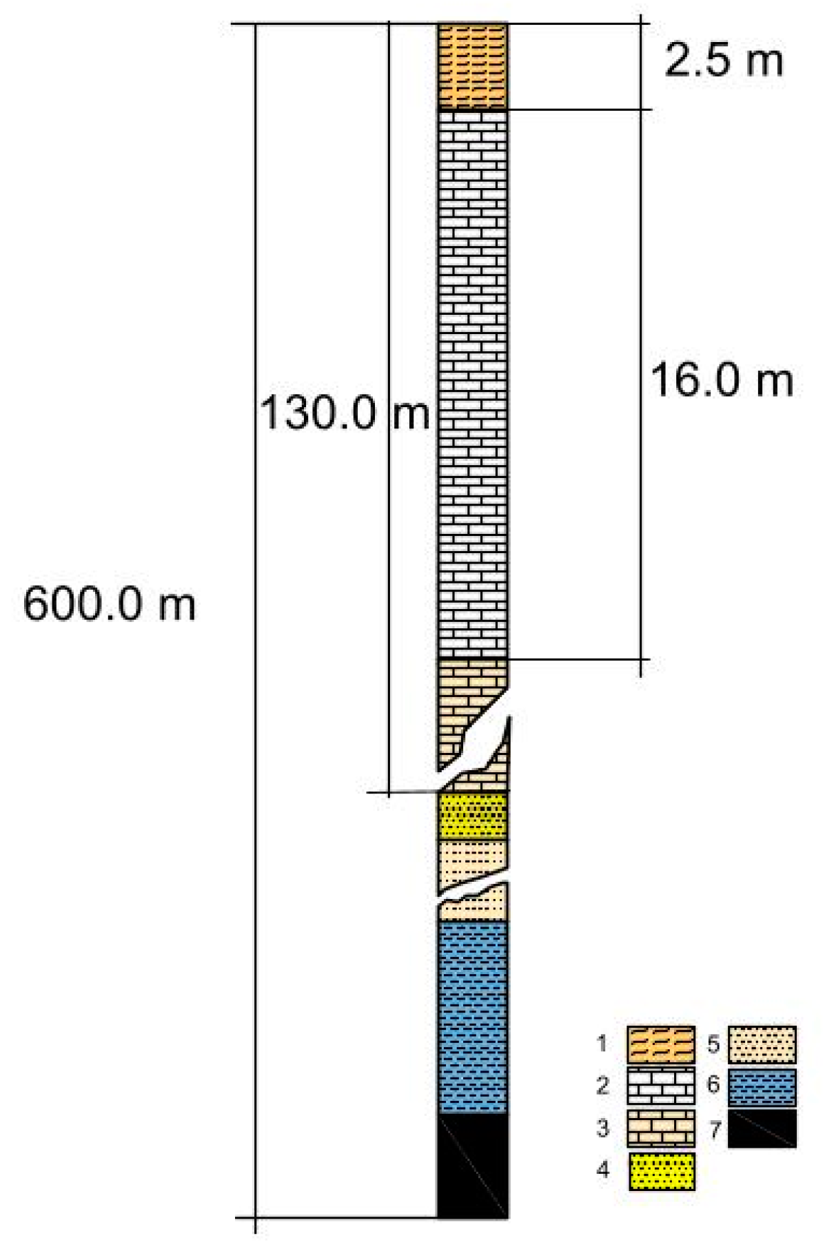
2.1. Rock Mass Structure

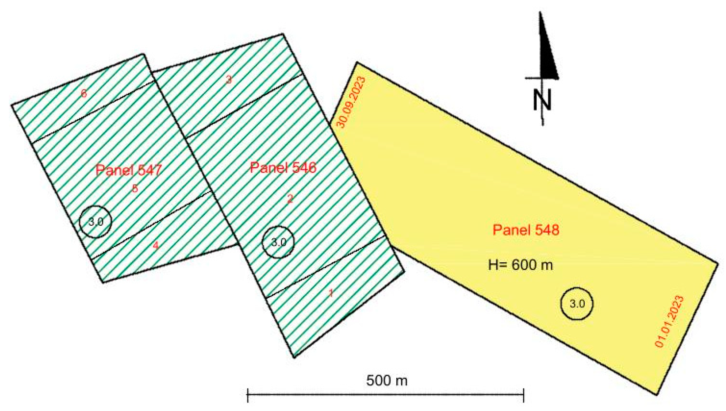
The rock mass in the study area was built of Quaternary and Triassic overburden strata and productive carbon. The overburden was formed during the Quaternary period from clay. The thickness of these formations ranges from 1.8 m to 2.5 m. Middle Triassic strata, made of limestones and dolomites, among others, are deposited underneath. These formations reach a depth of approximately 130 m. Below, there is carbon made of sandstone interbedded with coal seams. Carbon is made of Libiąż Beds with group 100 coal beds and of Łaziska Beds with group 200 coal bed. The subject of extraction in the area under consideration was coal bed 207. Seam thickness in the area of the chosen panels ranged from 4.2 m to 5.0 m along with locally occurring interlayers of 0.10 m to 0.18 m thick clay shale. In the roof of the bed, there are clay shales as well as fine-grained and medium-grained sandstones. The angle of the bed inclination in the extraction area ranged from 3.5° to 5.5°. Figure 1 shows a simplified lithological profile.

Based on the works [4,8], it is known that when strength of the layers building the rock mass increases, the range of subsidence trough also increases (the value of tan β parameter decreases). In the case of rock mass in Upper Silesia, the value of tan β parameter ranges from 1.5 to 2.5 depending on the strength properties of the rock mass. The structure of the rock mass also influences the course of subsidence over time. In a rock mass built of high-strength rocks, the course of subsidence is slower than in a rock mass of lower strength. The results of research conducted so far do not indicate the influence of the rock mass properties on the value of the coefficient of roof control a.

2.2. Coal Mining

Mining extraction was conducted with caving of the roof of 3 m high in the 207 coal seam along two panels: 546 and 547. In order to carry out the calculations with the greatest possible accuracy, the panels were divided into lots 1–6 determined by the quarterly progress of extraction.

Table 1. Basic information about the extraction.

Seam/Panel	Start	End	H, m
546/1	1 December 2017	31 December 2017	597
546/2	1 January 2018	31 March 2018	580
546/3	1 April 2018	1 July 2018	565
547/4	1 September 2018	30 September 2018	575
547/5	1 October 2018	31 December 2018	565
547/6	1 January 2019	1 March 2019	557

shows basic data on the completed extraction, along with the depth of the deposition of strata in the area of lot-H.

In the analyzed region, further longwall mining is planned along the 548 panel at the height of 3 m with the roof fall at the average depth of 600 m.

Figure 2 shows the location of completed and planned extractions. It shows the division of the 546 and 547 panels into lots 1–6. Planned longwall mining along the 548 panel is shaded yellow.

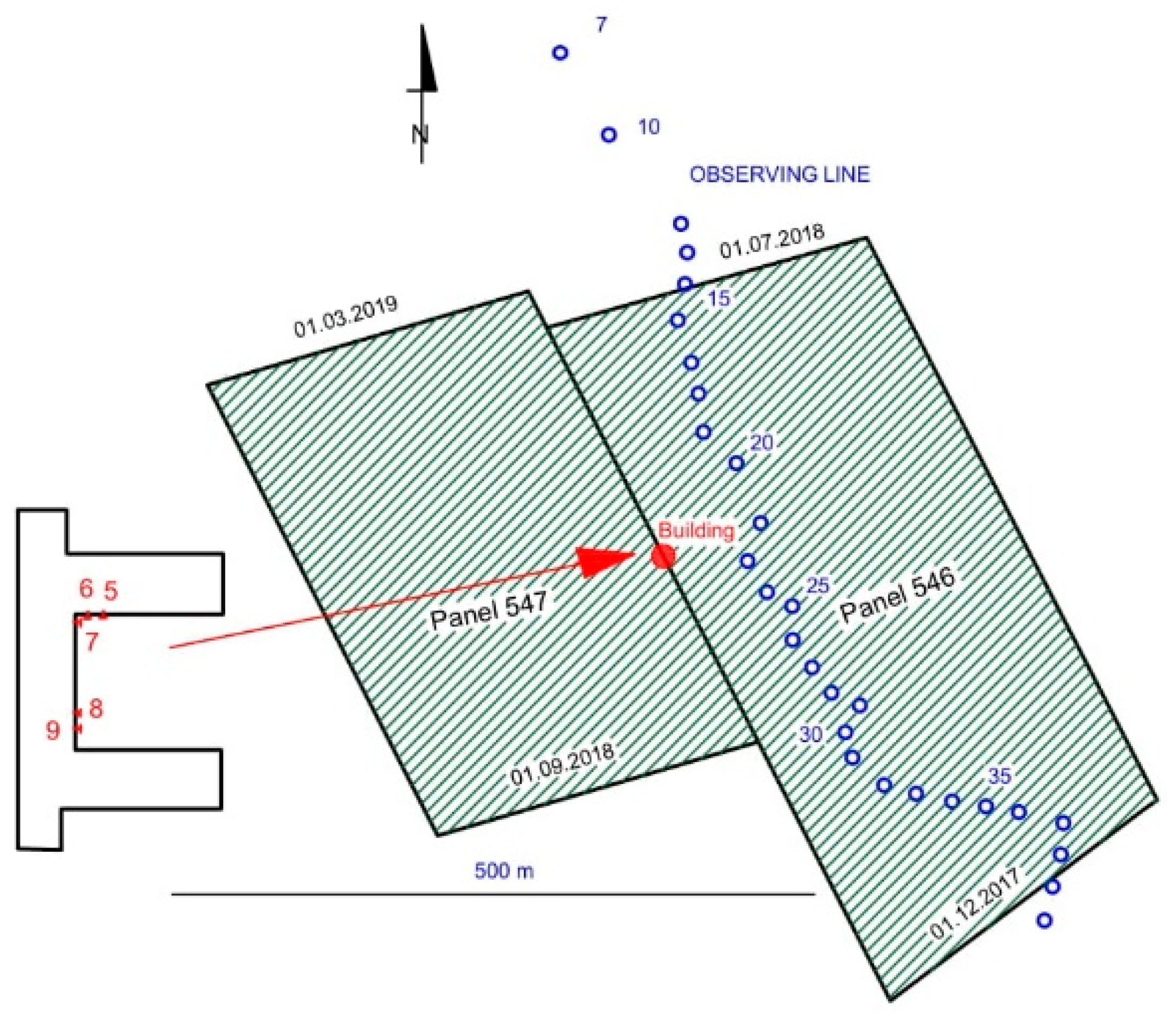
2.3. Land Surveying and Results

The impact of extraction on the surface was monitored by measurements carried out along the observation line consisting of benchmarks in the ground and wall benchmarks fixed on the building. The locations of monitoring points were set along with the actual topography on the ground surface including a street located on the ground surface above panel 546. The measurements were conducted every six months between April 2017 and July 2020. The location of the building (red mark) and measurement line are shown in Figure 3.

Subsidence of the line benchmarks is shown in Figure 4, and the wall benchmarks in Figure 5. It can be seen from these figures that the area has not subsided since March 2020. Some benchmarks were indeed subsidence in the last measurement, but in the previous ones they were raised, which proves measurement errors. More accurate measurement results based on the wall benchmarks confirm that the lowering process ended in March 2020.

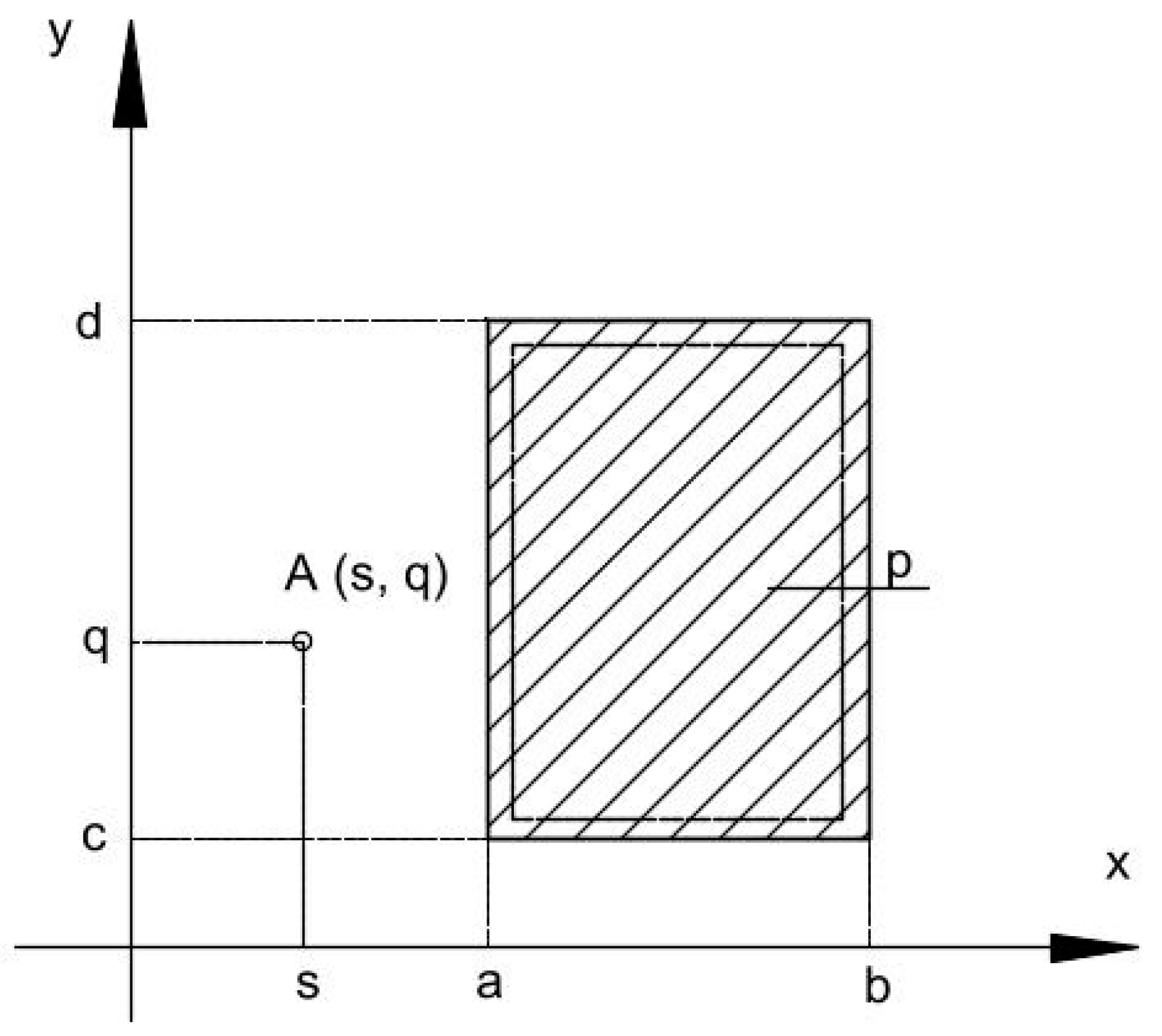
2.4. Analysis Method Used

The Budryk–Knothe theory (Knothe 1983) was used for the analysis conducted in this paper due to its huge popularity in Poland [4,24,25] and in other countries [5,11,18,26,27]. Despite this popularity, it is worth providing the basic formulas for the extraction field of a rectangular shape. Longwall workings most often have a rectangular shape. Moreover, each polygon can be approximated with elementary rectangles, similar to integration by the rectangle method. Assuming a rectangular coordinate system of 0XY and point A (s, q)—Figure 6, Knothe provided a formula for subsidence of a point:

$$\mathrm{w}\left(\mathrm{s},\mathrm{q}\right)=\frac{{\mathrm{w}}_{\max }}{{\mathrm{r}}^2}{{\displaystyle \int }}_{\mathrm{a}-\mathrm{s}}^{\mathrm{b}-\mathrm{s}}{\mathrm{e}}^{\frac{-{\mathsf{\pi }\mathsf{\xi }}^2}{{\mathrm{r}}^2}}\mathrm{d}\mathsf{\xi }{{\displaystyle \int }}_{\mathrm{c}-\mathrm{q}}^{\mathrm{d}-\mathrm{q}}{\mathrm{e}}^{\frac{-{\mathsf{\pi }\mathsf{\xi }\mathsf{\eta }}^2}{{\mathrm{r}}^2}}\mathrm{d}\mathsf{\eta }$$

(1)

where:

• ξ = x − s,

• η = y − q.

Taking into consideration the peripheral area p, the edges of mining should be shifted by its value in the directions shown in the figure, which is taken into account in the integration limits.

In Formula (1), the following parameters of the theory can be distinguished:

• Exploitation coefficient (of roof control)—a, dimensionless quantity. Its value depends on the method of liquidation of the selected part of the deposit. In the Upper Silesian Coal Basin, for caving mining the values are a = 0.7–0.9;
• Main impact radius r, expressed in meters. This parameter is used interchangeably with the parameter tan β, where β is the angle of the reach of the main impact.

Both of these parameters are related to each other:

$$\tan \mathsf{\beta }=\frac{\mathrm{H}}{\mathrm{r}}$$

(2)

where H—depth of extraction, m;

• Extraction periphery is an additional parameter in the theory-p.

In the Upper Silesian Coal Basin (Poland), usually (routinely) the value a = 0.8 (extraction with the roof fall) and tan β = 2 are used for calculations. The value of the periphery is estimated at 0.14 r–0.20 r.

The remaining deformation indices are calculated as depression derivatives in accordance with the following dependencies.

The slopes in the X and Y directions are shown in the formula:

$${\mathrm{T}}_{\mathrm{x}}=\frac{\partial \mathrm{w}}{\partial \mathrm{x}},{\mathrm{T}}_{\mathrm{y}}=\frac{\partial \mathrm{w}}{\partial \mathrm{y}}$$

(3)

The maximum slope is shown by the formula:

$${\mathrm{T}}_{\max }=\left|\mathrm{grad}\mathrm{w}\left(\mathrm{x},\mathrm{y}\right)\right|=\sqrt{{\mathrm{T}}_{\mathrm{x}}^2+{\mathrm{T}}_{\mathrm{y}}^2}$$

(4)

Vertical curves in the direction of the X and Y axes are shown by the formula:

$${\mathrm{K}}_{\mathrm{x}}=\frac{{\partial }^2\mathrm{w}}{\partial {\mathrm{x}}^2},{\mathrm{K}}_{\mathrm{y}}=\frac{{\partial }^2\mathrm{w}}{\partial {\mathrm{y}}^2}$$

(5)

Horizontal shifts in the direction of the X and Y axes are shown by the formula:

$${\mathrm{u}}_{\mathrm{x}}=-\mathrm{B}·{\mathrm{T}}_{\mathrm{x}},{\mathrm{u}}_{\mathrm{y}}=-\mathrm{B}·{\mathrm{T}}_{\mathrm{y}},$$

(6)

Horizontal deformations in the direction of the X and Y axes are shown by the formula:

$${\epsilon }_{\mathrm{x}}=\mathrm{B}\cdot \frac{{\partial }^2\mathrm{w}}{\partial {\mathrm{x}}^2},{\epsilon }_y=\mathrm{B}\cdot \frac{{\partial }^2\mathrm{w}}{\partial {\mathrm{y}}^2}$$

(7)

where:

B = 0.32 r

Horizontal deformations in the direction of the main axes are shown by the formula:

$${\mathsf{\epsilon }}_{1,2}=0.5·\left({\mathsf{\epsilon }}_{\mathrm{x}}+{\mathsf{\epsilon }}_{\mathrm{y}}\right)\pm \sqrt{0.25·{\left({\mathsf{\epsilon }}_{\mathrm{x}}-{\mathsf{\epsilon }}_{\mathrm{y}}\right)}^2+0.5·{\mathsf{\gamma }}_{\mathrm{xy}}^2}$$

(8)

where:

γ_xy—complete differential:

$${\mathsf{\gamma }}_{\mathrm{xy}}=\frac{\partial {\mathrm{u}}_{\mathrm{x}}}{\partial \mathrm{y}}+\frac{\partial {\mathrm{u}}_{\mathrm{y}}}{\partial \mathrm{x}}$$

(9)

Maximum horizontal deformations-εmax are understood as the maximum absolute value with ε1 and ε2. On the other hand, the values of deformation indicators are grouped into categories of mining areas, which are shown in

Table 2. Categories of mining areas depending on the values of deformation indicess.

Category	T, mm/m	R, 1/km	ε, mm/m
0	T ≤ 0.5	40 ≤ │R│	│ε│ ≤ 0.3
I	0.5 < T ≤ 2.5	20 ≤ │R│ < 40	0.3 < │ε│ ≤ 1.5
II	2.5 < T ≤ 5	12 ≤ │R│ < 20	1.5 < │ε│ ≤ 3.0
III	5 < T ≤ 10	6 ≤ │R│ < 12	3.0 < │ε│ ≤ 6.0
IV	10 < T ≤ 15	4 ≤ │R│ < 6	6.0 < │ε│ ≤ 9.0
V	T > 15	│R│ < 4	|ε| > 9

. The categories of building structures resistance are compared to the mining area categories given in Table 2. If the area category does not exceed the category of the building resistance, then the area is not threatened with damage.

To calculate the values of deformation indices at a given time t, Knothe [28] proposed an equation:

$$\frac{\mathrm{dw}}{\mathrm{dt}}=\mathrm{c}\left({\mathrm{w}}_{\mathrm{k}}-\mathrm{w}\left(\mathrm{t}\right)\right)$$

(10)

where:

• w(t)—temporary subsidence,
• w_k—asymptotic (final) subsidence,
• c—subsidence rate coefficient (time), 1/year or 1/day. According to S. Knothe [28], for the Upper Silesian Coal Basin c = 0.5–7, 1/year

To facilitate the calculations, it is assumed that c = const and w_k = const. Accepting the initial condition w(t = 0) = 0 provides a simple solution of Equation (10) as:

$$\mathrm{w}\left(\mathrm{t}\right)={\mathrm{w}}_{\mathrm{k}}·\left(1-{\mathrm{e}}^{-\mathrm{ct}}\right)$$

(11)

Using Equation (11) is possible with the discretization of calculations–dividing the panel area into small (elementary) panels, which can be assumed to have been extracted in a short time. Then, the subsidence caused by the exploitation of elementary (rectangular) panels is summed up at the given moment t, taking into account Equation (11). In this way, the changes in final subsidence w_k related to the expansion of exploitation field are taken into account.

The computer program DEFK-Win5.0 developed by Ścigała [29,30] worked on the above assumptions.

The program allows to make calculations for any number of panels in shape of any polygon. The area of the panels is approximated by elementary rectangles (similar to the integration using the rectangle method). The calculations are made using the Budryk–Knothe theory (see Formula (1) and following). Calculations can be performed for selected points on the surface or inside the rock mass. Performing calculations in a grid of points enables drawing of isoline maps of deformation indices. The program also enables identification of parameter values based on the measurement results of the final subsidence (parameters: a, tan β, p) and on the basis of values of subsidence in transient state (parameter c). The minimalization of goal function resulting from the smallest squares method is performed using the Hooke-Jeeves method.

3. Results

The analysis of land surveying results was conducted in order to identify the parameter values of S. Knothe theory, in order to use them to predict the state of deformation that would occur as a result of planned longwall extraction along the 548 panel. The analysis was conducted in stages:

-

identification of the parameter values: a, p, tan β on the basis of final subsidence registered on the measurement line section;

-

identification of parameter c value based on the lowering of the point over time.

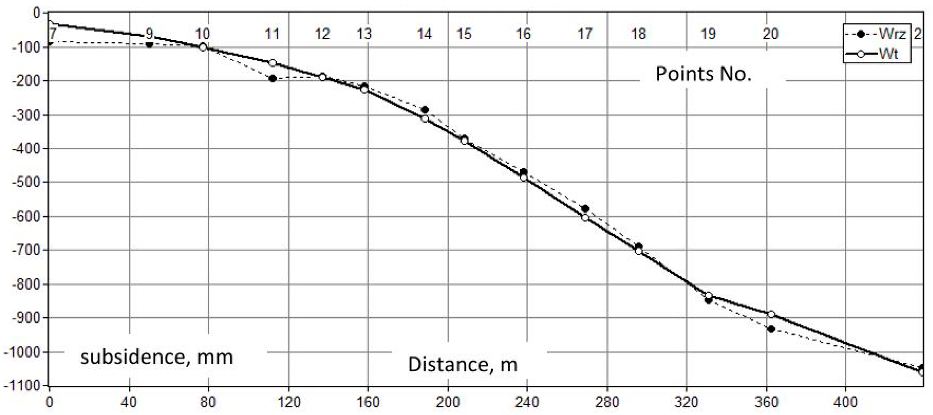
3.1. Identification of Parameter Values on the Basis of Determined Subsidence

In order to identify the parameter values of the Budryk–Knothe theory based on the land surveying results conducted on the observation line, the values recorded in the last measurement were taken as the final subsidence. Computer program DEFK-Win5.0 was used for the calculations [28].

The following parameter values were obtained:

p = 39.5 m, a = 0.517 tan β = 1.71.

Table 3. The comparison of calculated subsidence depressions including the peripheral areas and measurements.

Pkt	X	Y	wrz	wt	V	VV	sumV	sumVV
7	340.0	895.0	−86.0	−32.4	−53.6	2875.2	53.6	2875.2
9	370.0	855.0	−91.0	−67.7	−23.3	542.6	76.9	3417.8
10	380.0	830.0	−98.0	−100.2	2.2	4.8	79.1	3422.6
11	405.0	805.0	−194.0	−145.6	−48.4	2344.1	127.5	5766.7
12	420.0	785.0	−187.0	−189.1	2.1	4.6	129.7	5771.3
13	435.0	770.0	−216.0	−226.4	10.4	109.0	140.1	5880.3
14	435.0	740.0	−286.0	−311.6	25.6	657.1	165.7	6537.4
15	435.0	720.0	−371.0	−377.3	6.3	39.4	172.0	6576.8
16	435.0	690.0	−469.0	−486.3	17.3	298.1	189.3	6875.0
17	440.0	660.0	−579.0	−603.3	24.3	592.8	213.6	7467.8
18	450.0	635.0	−688.0	−700.8	12.8	164.7	226.5	7632.5
19	450.0	600.0	−848.0	−834.8	−13.2	175.0	239.7	7807.5
20	475.0	580.0	−931.0	−888.9	−42.1	1773.1	281.8	9580.6
23	485.0	505.0	−1047.0	−1060.5	13.5	181.5	295.3	9762.0

Standard deviation: 21.09 mm Percentage error: 2.62%. Explanations to the table: Pkt—point number; X, Y—coordinates of the point in the locally adopted Cartesian system, m; wrz—subsidence confirmed by the measurement, mm; wt—calculated subsidence, mm; V—difference between the values wt and wrz, mm; VV—square of difference v, mm²; SumV—sum of difference V, mm; SumVV—sum of squares of difference VV, mm².

shows the comparison of calculated subsidence with subsidence based on land surveying. A graphical comparison of subsidence depressions is shown in Figure 7.

Obviously, it should be borne in mind that the obtained parameter values are unusual in comparison to those that are commonly used. Nevertheless, they are confirmed by the analyses carried out earlier for the same part of the basin. The results of the previous analyses are shown in Figure 8. As can be seen in the figure, with the increase in the value of the parameter tan β, the value of the parameter a also increased. The value of the parameter tan β is related to the mechanical properties of the rock mass. The higher the rock mass strength parameters, the lower the value of tan β. Thus, with subsequent extractions, the parameter value decreased. Figure 8 illustrated the analysis results—values a and tan β obtained as a result of determination based on the measurement results, the linear relationship between them as:

a = 0.6395 tan β − 0.6338

(12)

as well as the confidence intervals at the level of 0.95.

The value of the correlation coefficient R = 0.88 was obtained.

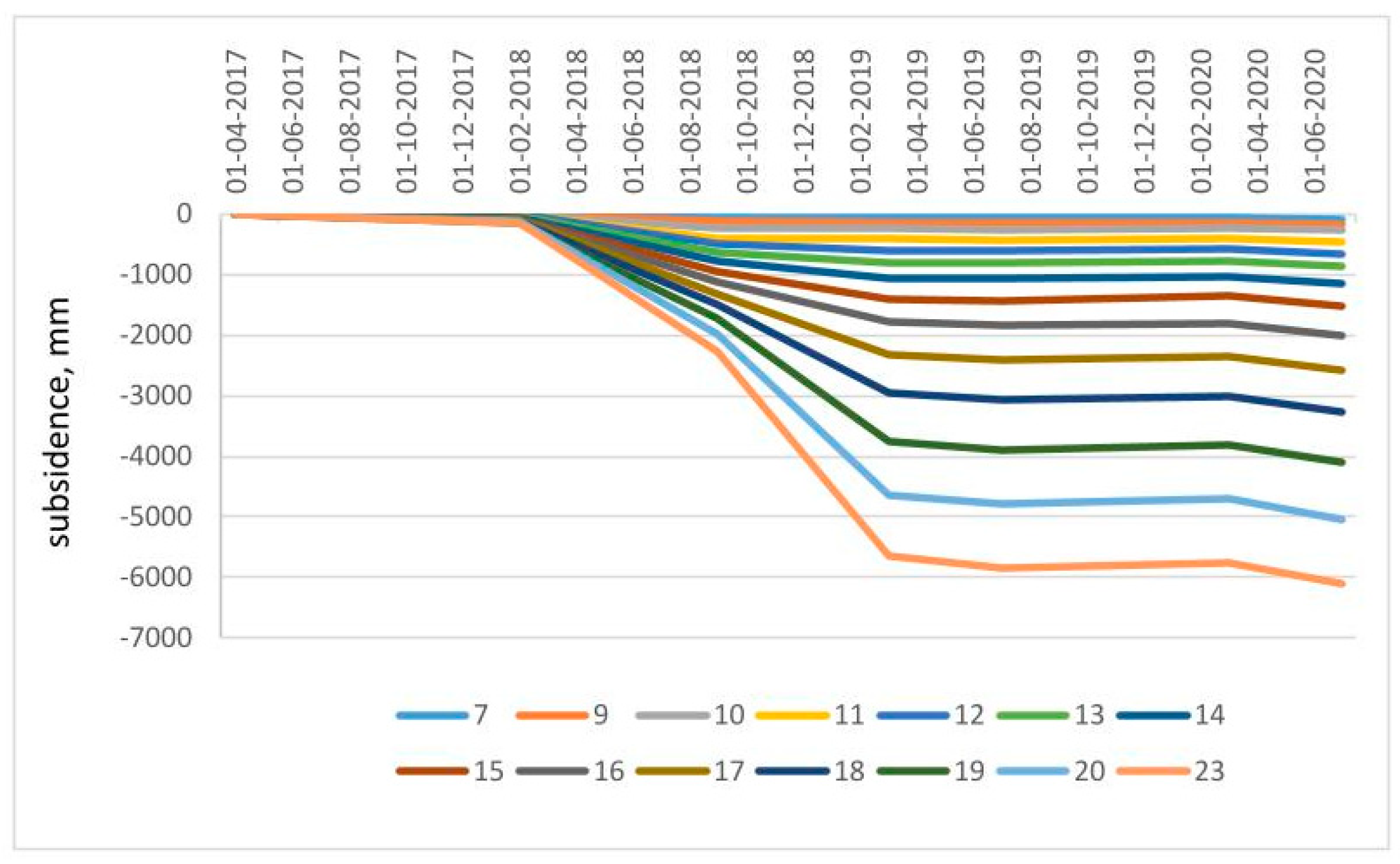
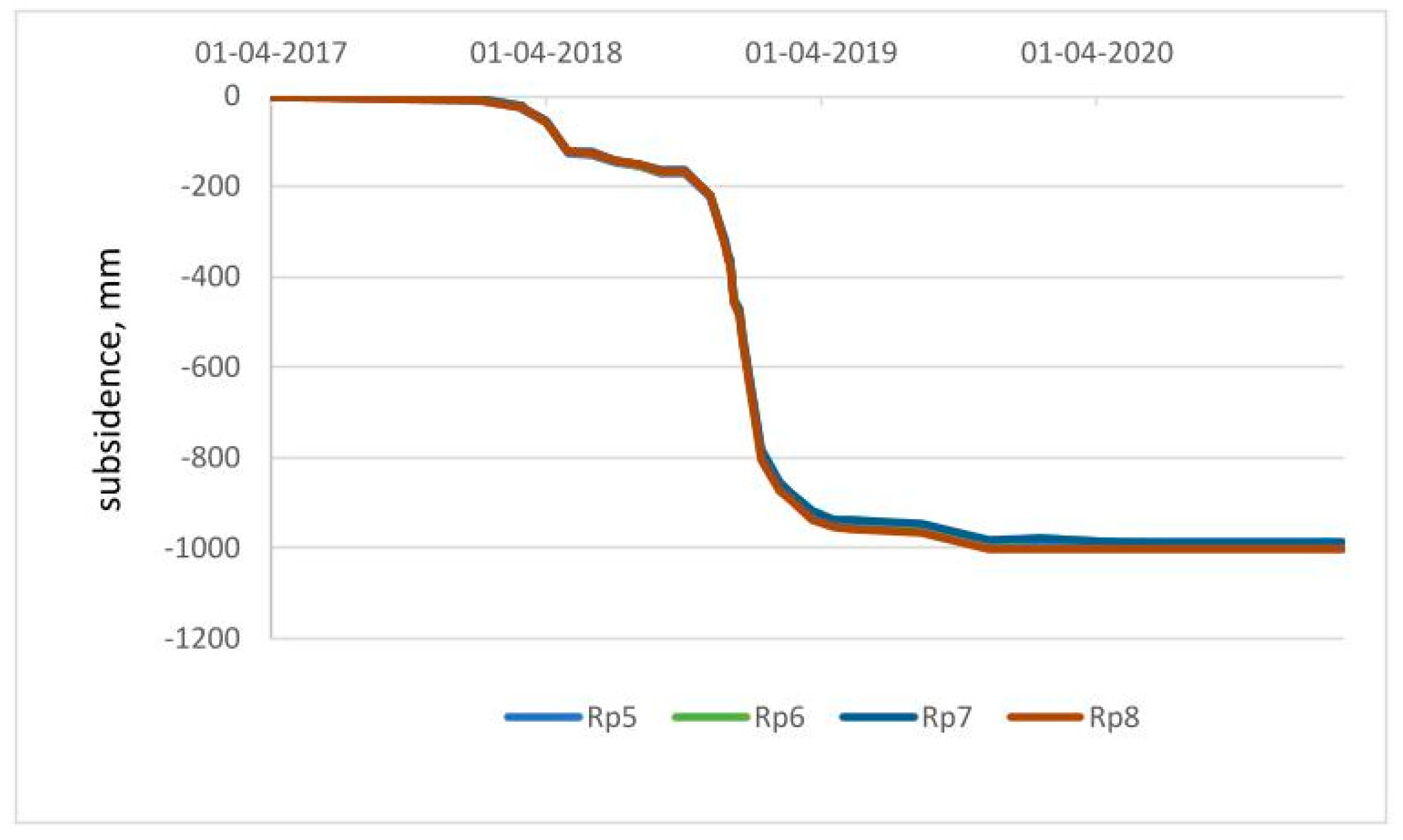
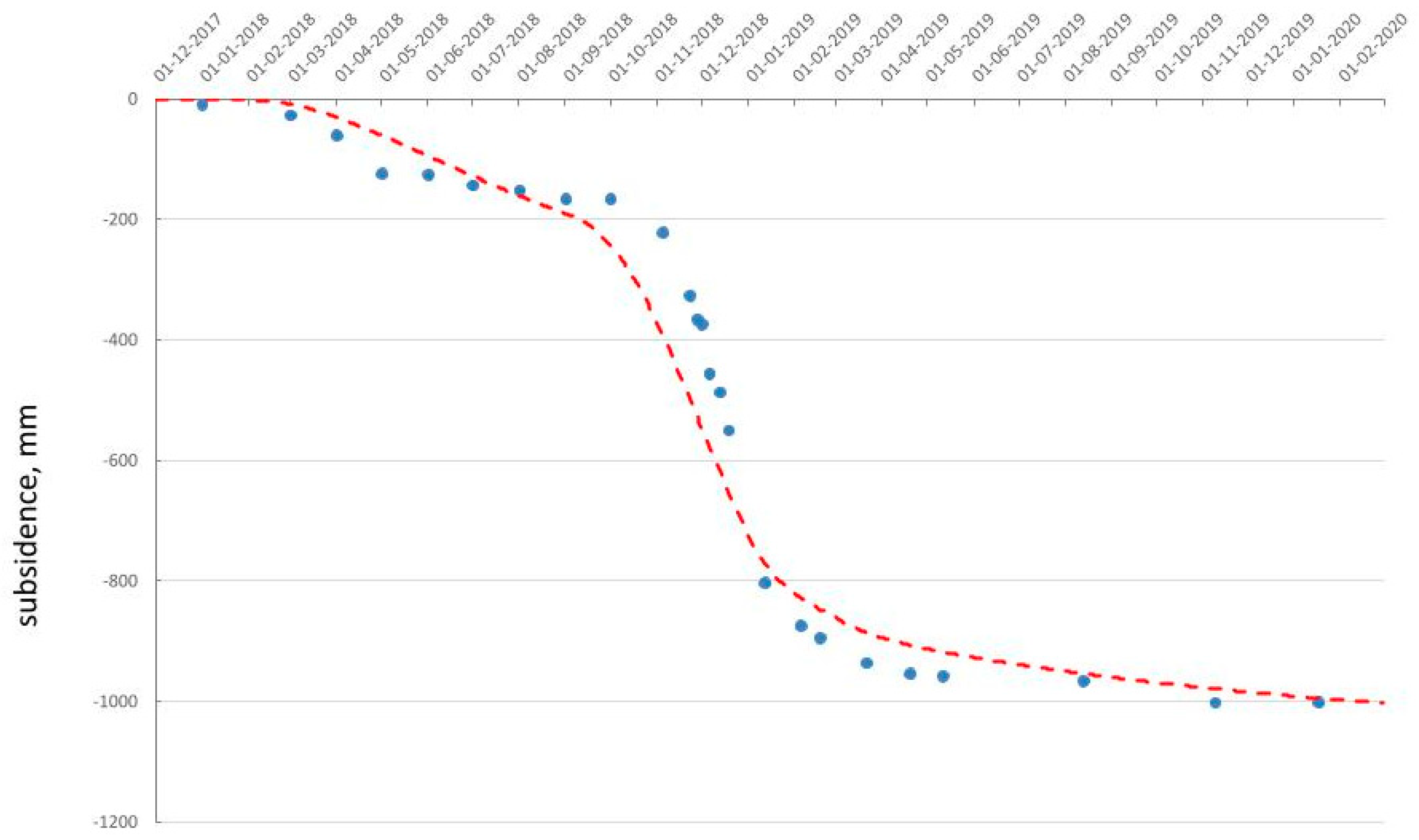
3.2. Identification of Subsidence Rate Coefficient

The identification of subsidence rate coefficient c was conducted based on the subsidence in the wall benchmark no. 8 stabilized on the building. The calculations were performed for one point due to the high repeatability of the measurement results obtained in points 5–8 (see Figure 5). As can be seen in Figure 5, a high repeatability of wall benchmarks subsidence was confirmed by measurements. The benchmark fixed on the building was selected for the analyses due to a higher accuracy of measurements than those carried out on the benchmarks set on the ground. Figure 9 illustrates the results of measurements with red bullet points, and the graph of calculated subsidence with a dashed line. The calculations were made using computer program DEFK-Win. In the case of the 546 panel, the obtained value was c = 0.003 1/day, and for the 547 panel c = 0.05 1/day.

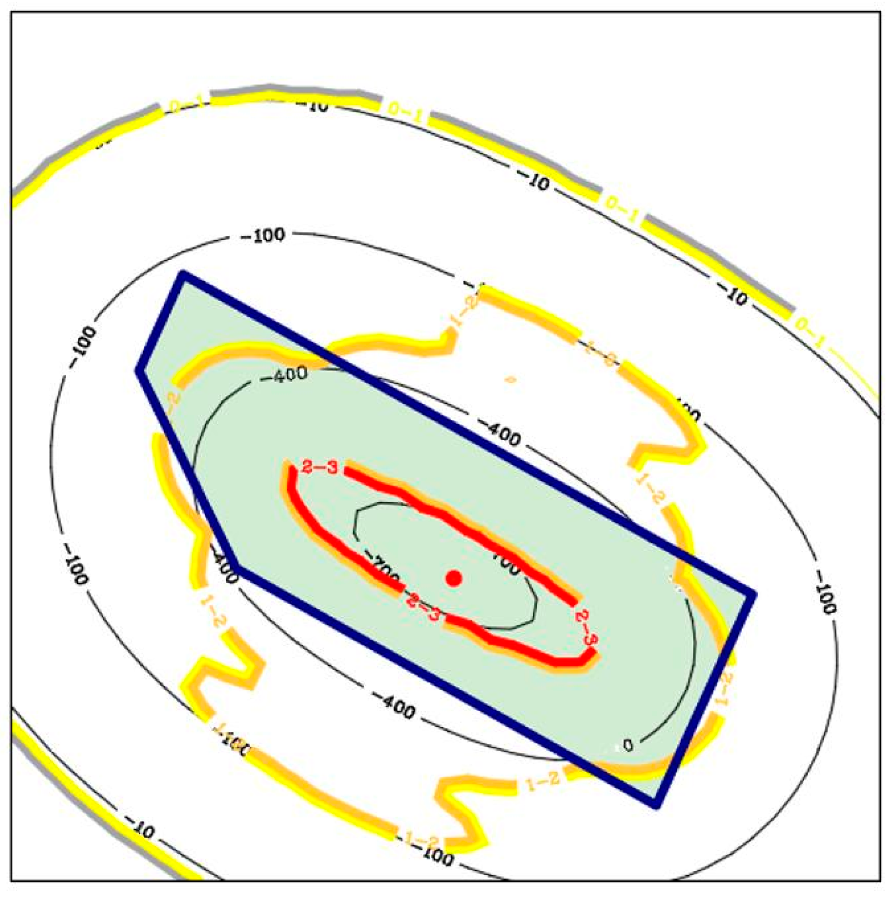
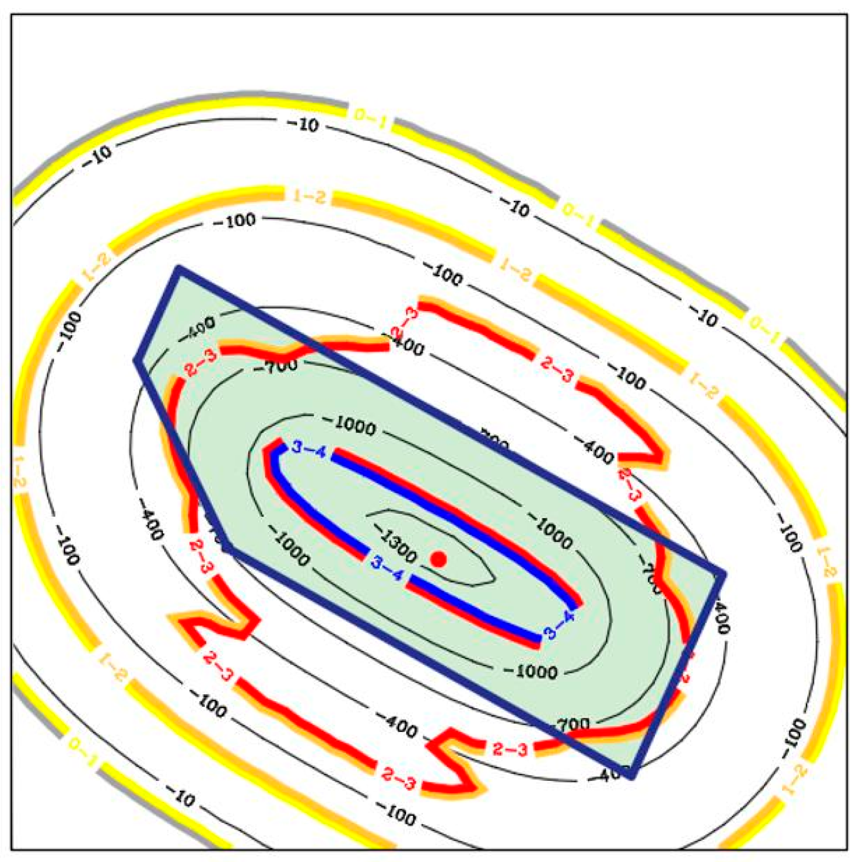
3.3. Prediction of Ground Deformation As a Result of Planned Extraction

The calculations were made for the final state of deformations that would occur once the extraction of the 548 panel ended. The assumptions for the predictions of the impacts of the 548 panel extraction on the surface were made based on the above-mentioned analyses of the measurement results. The following parameter values were adopted:

Variant 1

-

exploitation coefficient a = 0.517;

-

tangent of the range of main impacts tan β = 1.71;

-

extraction periphery p = 40 m.

The calculation results are presented in the form of a graphic map of subsidence isolines as well as mining areas categories resulting from maximum slopes and maximum horizontal strains. Figure 10 illustrates the boundaries of extraction of the 548 panel and isolines of predicted subsidence and areas subject to deformations within the range of individual categories. These areas are marked with appropriate colours and are illustrated with appropriate numbers.

For comparison, identical calculations were also made adopting standard, commonly accepted parameter values:

Variant 2

-

exploitation coefficient a = 0.800;

-

tangent of the range of main impacts tan β = 2.00;

-

extraction periphery p = 40 m.

The calculation results are graphically illustrated in Figure 11, using analogous markings as in Figure 10.

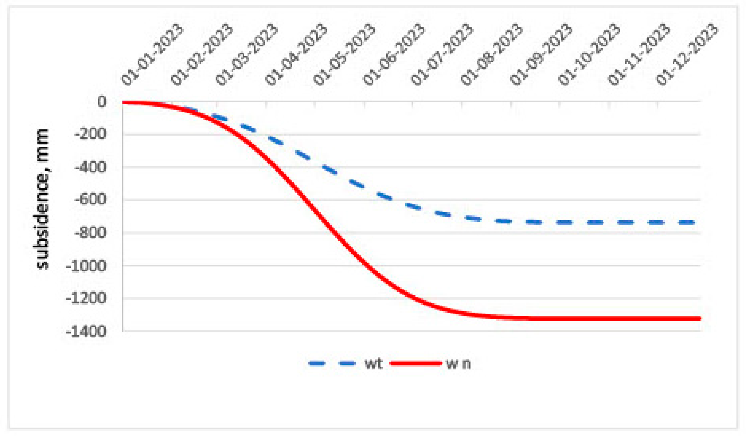
3.4. Detailed Forecast for the Selected Object

Detailed calculations were carried out for a selected point above the planned extraction of the 548 panel. A computer simulation of the wall run was performed using DEK-Win 5.0 software. This point is marked in red in Figure 10 and Figure 11. Similarly to the calculations done before, they were performed for two sets of parameters:

A variant–the calculations were made assuming a delay in the impact of mining, according to formula (11). The following parameter values were adopted:

-

exploitation coefficient a = 0.517;

-

tangent of the range of main impacts tan β = 1.71;

-

extraction periphery p = 40 m;

-

subsidence rate coefficient c = 0.05 1/day.

B variant–the calculations were made assuming immediate impact of mining, adopting standard parameter values:

-

exploitation coefficient a = 0.800;

-

tangent of the range of main impacts tan β = 2.00;

-

extraction periphery p = 40 m;

-

c -> ∞.

In other words, in the case of variant B, the subsidence at a given time t is equal to the final value of the subsidence caused by the extraction performed up to that time. In the case of variant A, the value of subsidence at time t is obviously smaller, which results from the Equation (11). In the case of variant A, the subsidence reaches the final value corresponding to the range of exploitation carried out until time t only after time T > t. Of course, the calculations according to both variants were performed with very different values of parameters a and tan β. Variant A reflects a case more similar to the actual state, both due to the inclusion of the time variable and the parameter values obtained on the basis of the measurement results.

Figure 12 shows the graphs of subsidence. Subsidence for A variant is marked with a blue line and wt symbol, whereas B variant is marked with a red line and wn symbol.

Figure 13 shows the graphs of maximum slopes. The slopes for A variant are marked with a blue line and Tmax t symbol, whereas for B variant are marked with a red line and Tmax n symbol.

Figure 14 illustrates the graphs of maximum horizontal strains. The strains for A variant are marked with a blue line and Emax t symbol, whereas for B variant are marked with a red line and Emax n symbol.

4. Discussion

The determination of the parameter values of the Budryk–Knothe theory based on the final trough enabled to obtain a high consistency between the calculation results and the results of subsidence measurements. This is indicated by the obtained subsidence percentage error value amounting to 2.62%—Table 3, Figure 7. It should be emphasized that the exploitation coefficient a = 0.517 is unusually low. As noted in point 2 of this paper, this value was expected to range between 0.7 and 0.9. The reason for this should be seen in the geological structure of the rock mass, i.e., high depth of strong limestone rocks of which the cover was made [31]. This corresponds with the obtained parameter value tan β = 1.71, which is characteristic of high-strength rocks [4]. In the case under consideration, not only a low value of the parameter tan β, but also of the parameter a were obtained. The correctness of the obtained results of the analyses is confirmed by the results of the previous research–Figure 8. It should be assumed that in the initial period of extraction, the parameter values a and tan β are low, and subsequently, as further extraction is carried out, they increase to the values commonly used for predictions.

The calculated subsidence of the selected point over time corresponds to the measurement results—Figure 9. Subsidence caused by the extraction of the 546 panel appeared slowly on the surface, as evidenced by the obtained value of the coefficient c = 0.003 1/day. Taking into account the above-described rock mass structure and the lack of earlier instances of mining in the immediate vicinity, such a small value is plausible. During the extraction of the 547 panel, the value c was higher and equaled c = 0.05 1/day, which should be explained by a greater degree of rock mass loosening as a result of the extraction of the 546 panel.

The following facts can be observed based on the prediction of the final state of deformations induced by the planned extraction of the 548 panel, which was conducted in the next stage of this work. Taking the parameter values obtained on the basis of the measurement results for calculations (Figure 10, variant 1) enabled the values of maximum subsidence of approximately 0.75 m and maximum deformations from the 3rd category to be obtained.

Taking the standard, commonly used parameter values for calculations (Figure 11, variant 2) resulted in obtaining much higher subsidence values equaling to 1.3 m and maximum deformations from the 4th category. As long as the occurrence of deformations in the 3rd category is accepted by local government authorities, the deformations of the 4th category mean that planned extraction under built-up areas would not be granted a permit from these authorities. Therefore, the importance of issues related to predictions of the state of deformations to truly reflect the actual state and the consequences it has, is clear.

In the paper, the need to make predictions of the deformation state, taking into account their course over time, was also considered. Such predictions are usually made for building structures of higher importance. A sample prediction was made for the object marked with a red circle in Figure 10 and Figure 11. The calculations were carried out by making a computer simulation of the run of the workings. Similarly to the previous instance, we took the parameter values for the immediate effects (variant A) and for the delayed effects, according to Equation (11)—variant B. Here, of course, significant differences in the deformation state can also be observed. Subsidence illustrated in Figure 12 differed almost twice. Taking into account the parameters obtained based on the measurement results, the maximum slope was approximately 2 mm/m (1st category), whereas taking the typical parameter values and the immediate effects, they equaled to approximately 4.3 mm/m (2nd category)—Figure 13. Even greater differences occurred in the case of horizontal strains. Considering the parameters obtained based on the measurements results, the values of deformations were approximately +0.9 mm/m (1st category) and approximately −3.9 mm/m (3rd category), whereas considering typical parameter values and the immediate effect, they were approximately +2 mm/m (2nd category) and approximately −7.1 mm/m (4th category)—Figure 14. Of course, the course of deformation over time is very important information for construction specialists, who determine the possibility of damage occurrence to objects.

Figure 15 shows graphs of extracted and possible to extract bituminous coal resources as a result of properly conducted predictions. The resources are divided into lots 1–6 and the 548–7 panels. All the resources account for 820 500 Mg of coal.

5. Conclusions

Based on the analyses conducted in this paper, the following conclusions and statements can be made:

• Geological and mining conditions, including the structure of the rock mass, have a significant impact on the parameter values necessary for the preparation of mining area deformation predictions. In cases where these conditions differ significantly from the average ones in a given area, it is particularly important to identify the parameter values based on the measurement results. Taking typical parameter values significantly influences the quality of the calculation results and leads to wrong conclusions about possible damage to buildings. Consequently, it leads to wrong decision-making regarding the possibility of conducting a planned mining extraction:
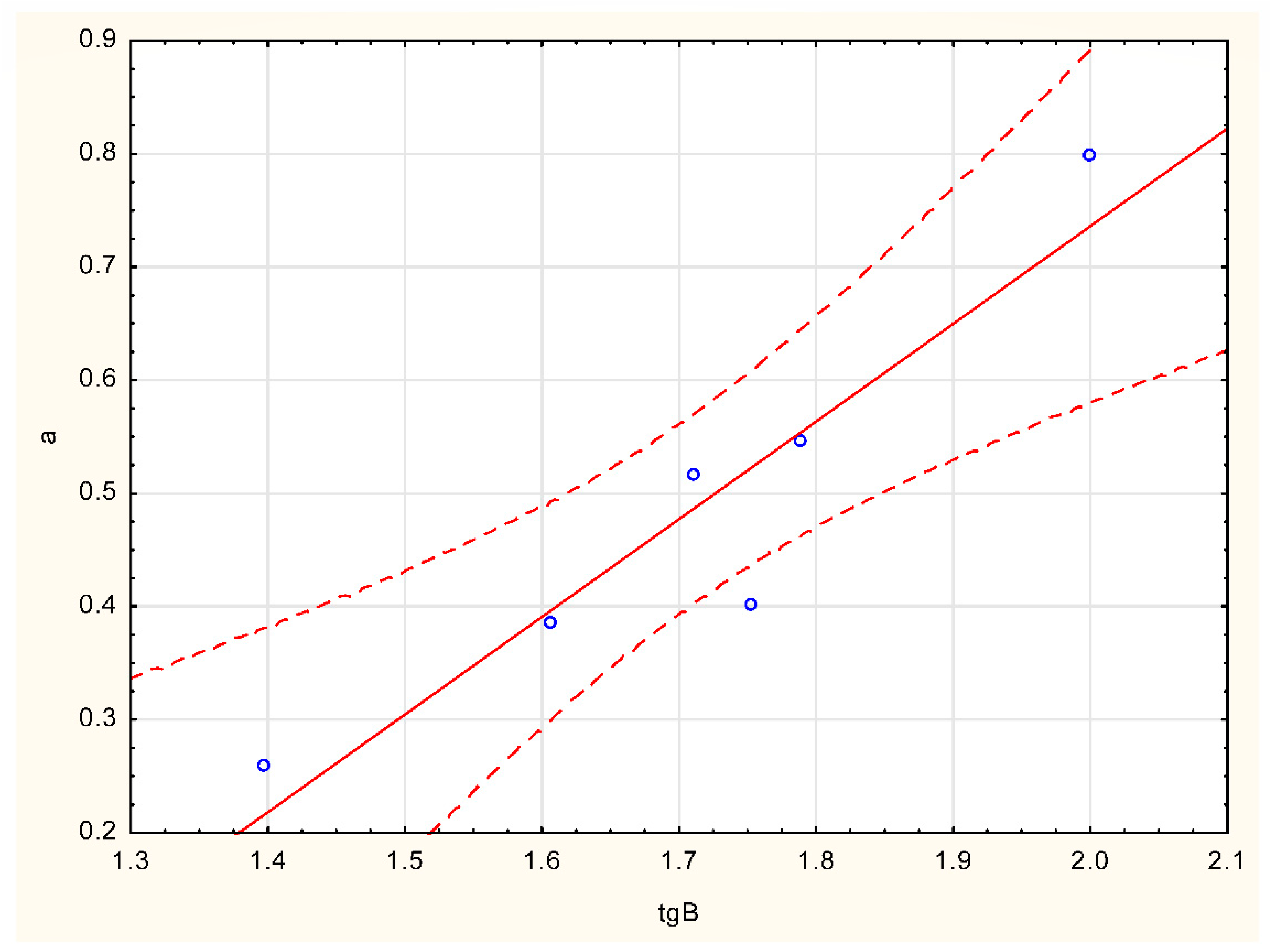
• In unusual geological conditions, when the overburden is made of strong limestone rocks, preliminary research indicated a gradual increase in the values of and tan β parameters up to the values commonly used for predictions. The previous experience has implied the influence of rock mass mechanical properties on the value of tan β parameter. Based on the research results presented in this paper it is clear that there is also a correlation between the values of the coefficient of roof control and the values of tan β, which are dependent on the rock mass structure. When analyzing the impact of planned extraction on more important objects, predictions should take into account the parameter values obtained during land surveying for specific geological and mining conditions. Such predictions should take into account a delay in the impacts, e.g., according to Equation (11).

References

1. Strzałkowski, P.; Litwa, P. Environmental protection problems in the areas of former mines with emphasis on sinkholes: Selected examples. Int. J. Environ. Sci. Technol. 2021, 18, 771–780. [Google Scholar] [CrossRef]
2. Guo, W.; Guo, M.; Tan, Y.; Bai, E.; Zhao, G. Sustainable development of resources and the environment: Mining—Induced eco-geological environmental damage and mitigation measures—A case study in the Henan coal mining area, China. Sustainability 2019, 11, 4366. [Google Scholar] [CrossRef] [Green Version]
3. Li, G.; Yang, Q. Prediction of Mining Subsidence in Shallow Coal Seam. Math. Probl. Eng. 2020, 2020, 7956947. [Google Scholar] [CrossRef]
4. Strzałkowski, P. Zarys Ochrony Terenów Górniczych; Wyd. Pol. Śl.: Gliwice, Poland, 2015. [Google Scholar]
5. Kratzsh, H. Mining Subsidence Engineering; Springer: Berlin/Heidelberg, Germany; New York, NY, USA, 1983. [Google Scholar]
6. Lee, F.T.; Abel, J.F., Jr. Subsidence from Underground Mining: Environmental Analysis and Planning Considerations; Geological Survey Circular, 876; United States Department: Washington, DC, USA, 1983. [Google Scholar]
7. Kwiatek, J. (Ed.) Ochrona Obiektów Budowlanych na Terenach Górniczych; Wydawnictwo Głównego Instytutu Górnictwa: Katowice, Poland, 1997. [Google Scholar]
8. Knothe, S. Prognozowanie Wpływów Eksploatacji Górniczej; Wydawnictwo Śląsk: Katowice, Poland, 1984. [Google Scholar]
9. Zych, J. Metoda prognozowania wpływów eksploatacji górniczej na powierzchnię terenu uwzględniająca asymetryczny przebieg procesu deformacji. Zesz. Nauk. Politech. Śląskiej 1987, 164, 17–19. [Google Scholar]
10. Li, J.; Wang, L. Mining subsidence monitoring model based on BPM-EKTF and TLS and its application in building mining damage assessment. Environ. Earth Sci. 2021, 80, 396. [Google Scholar] [CrossRef]
11. Zhu, X.; Guo, G.; Zha, J.; Chen, T.; Fang, O.; Yang, X. Surface dynamic subsidence prediction model of solid backfill mining. Environ. Earth Sci. 2016, 75, 1007. [Google Scholar] [CrossRef]
12. Zhao, B.; Guo, Y.; Mao, X.; Zhai, D.; Zhu, D.; Huo, Y.; Sun, Z.; Wang, J. Prediction Method for Surface Subsidence of Coal Seam Mining in Loess Donga Based on the Probability Integration Model. Energies 2022, 15, 2282. [Google Scholar] [CrossRef]
13. Yu, Y.; Ma, L.; Zhang, D. Characteristics of Roof Ground Subsidence While Applying a Continuous Excavation Continuous Backfill Method in Longwall Mining. Energies 2020, 13, 95. [Google Scholar] [CrossRef] [Green Version]
14. Vušović, N.; Vlahović, M.; Kržanović, D. Stochastic method for prediction of subsidence due to the underground coal mining integrated with GIS, a case study. Environ. Earth Sci. 2021, 80, 67. [Google Scholar] [CrossRef]
15. Chen, Q.; Li, J.; Enke, H. Dynamic simulation for the process of mining subsidence based on cellular automata model. Open Geosci. 2020, 12, 832–839. [Google Scholar] [CrossRef]
16. Chudek, M. Geomechanika z Podstawami Ochrony Środowiska Górniczego I Powierzchni Terenu; Wydawnictwo Politechniki Śląskiej: Gliwice, Poland, 2002. [Google Scholar]
17. Wesołowski, M. Numerical modeling of exploitation relics and faults influence on rock mass deformations. Arch. Min. Sci. 2016, 61, 893–906. [Google Scholar] [CrossRef] [Green Version]
18. Guzy, A.; Witkowski, W.T. Land Subsidence Estimation for Aquifer Drainage Induced by Underground Mining. Energies 2021, 14, 4658. [Google Scholar] [CrossRef]
19. Feng, Z.; Guo, W.; Xu, F.; Yang, D.; Yang, W. Control Technology of Surface Movement Scope with Directional Hydraulic Fracturing Technology in Longwall Mining: A Case Study. Energies 2019, 12, 3480. [Google Scholar] [CrossRef] [Green Version]
20. Zhang, B.; Ye, J.; Zhang, Z.; Xu, L.; Xu, N. A Comprehensive Method for Subsidence Prediction on Two-Seam Longwall Mining. Energies 2019, 12, 3139. [Google Scholar] [CrossRef] [Green Version]
21. Zhu, X.; Zhang, W.; Wang, Z.; Wang, C.; Li, W.; Wang, C. Simulation Analysis of Influencing Factors of Subsidence Based on Mining under Huge Loose Strata: A Case Study of Heze Mining Area, China. Geofluids 2020, 2020, 6357683. [Google Scholar] [CrossRef]
22. Peng, S.S. Coal Mine Ground Control, 3rd ed.; West Virginia University: Morgantown, WV, USA, 2008; p. 750. [Google Scholar]
23. Li, J.; Zhang, J.X.; Huang, Y.; Zhang, Q.; Xu, J.M. An investigation of surface deformation after fully mechanized, solid back fill mining. Int. J. Min. Sci. Technol. 2012, 22, 453–457. [Google Scholar] [CrossRef]
24. Orwat, J. Causes analysis of occurrence of the terrain surface discontinuous deformations of a linear type. International Conference on Applied Sciences. J. Phys. Conf. Ser. 2020, 1426, 012016. [Google Scholar] [CrossRef]
25. Orwat, J. Mining exploitation forecasted effects caused by a hard coal extraction from a thick seam. In Proceedings of the International Conference on Applied Sciences, Hunedoara, Romania, 9–11 May 2019. [Google Scholar] [CrossRef]
26. Whittaker, B.W.; Redish, D.J. Subsidence—Occurrence, Prediction and Control; Elsevier: Amsterdam, The Netherlands; Elsevier: Oxford, UK; Elsevier: New York, NY, USA; Elsevier: Tokyo, Japan, 1989. [Google Scholar]
27. Han, J.; Zou, J.; Hu, C.; Yang, W. Study on Size Design of Shaft Protection Rock/Coal Pillars in Thick Soil and Thin Rock Strata. Energies 2019, 12, 2553. [Google Scholar] [CrossRef] [Green Version]
28. Knothe, S. Wpływ czasu na kształtowanie się niecki osiadania. Arch. Min. Metall. 1953, 1, 51–62. [Google Scholar]
29. Ścigała, R. Komputerowe Wspomaganie Prognozowania Deformacji Górotworu i Powierzchni Wywołanych Podziemną Eksploatacją Górniczą; Wydawnictwo Politechniki Śląskiej: Gliwice, Poland, 2008. [Google Scholar]
30. Ścigała, R. The identification of parameters of theories used for prognoses of post mining deformations by means of present software. Arch. Min. Sci. 2013, 58, 1347–1357. [Google Scholar] [CrossRef] [Green Version]
31. Kryzia, K.; Majcherczyk, T.; Niedbalski, Z. Variability of exploitation coefficient of Knothe theory in relation to rock mass strata type. Arch. Min. Sci. 2018, 63, 767–782. [Google Scholar] [CrossRef]
Figure 1. Lithological profile of the borehole in the studied area. 1—clay, 2—limestone, 3—dolomite, 4—fine-grained sandstone, 5—medium-grained sandstone, 6—clay shale, 7—coal bed.
Energies 15 04627 g001
Figure 2. Diagram of mining location.
Energies 15 04627 g002
Figure 3. Location of the measurement line and building in relation to the extraction.
Energies 15 04627 g003
Figure 4. Subsidence of benchmarks in the ground over time.
Energies 15 04627 g004
Figure 5. Subsidence of wall benchmarks over time.
Energies 15 04627 g005
Figure 6. Diagram for Formula (1).
Energies 15 04627 g006
Figure 7. Measured and calculated final subsidence.
Energies 15 04627 g007
Figure 8. Relationship between the values of a and tan β parameters.
Energies 15 04627 g008
Figure 9. Measured and calculated subsidence for the benchmark no. 8.
Energies 15 04627 g009
Figure 10. Subsidence and categories of mining areas. Variant 1.
Energies 15 04627 g010
Figure 11. Subsidence and categories of mining areas. Variant 2.
Energies 15 04627 g011
Figure 12. Subsidence over time for A and B variants.
Energies 15 04627 g012
Figure 13. Maximum slopes over time for A and B variants.
Energies 15 04627 g013
Figure 14. Maximum horizontal strains over time for A and B variants.
Energies 15 04627 g014
Figure 15. Bituminous coal resources in individual lots.
Energies 15 04627 g015