Use of High-Frequency Ultrasound Waves for Boiler Water Demineralization/Desalination Treatment

Abstract

Isolated ultrasonic vibrations were used to treat feed water from a 20 bar steam-producing water tube boiler. Physical treatments such as ultrasounds and reverse osmosis (RO) are recommended as the most eco-friendly for this purpose. A novel bench-scale prototype delivering 6 L/h of treated water was designed and built. The ultrasonic atomization of raw water with 1.7 MHz piezoelectric transducers and subsequent humidification and dehumidification of drag airflow was the innovating sequence of operations used as a treatment technique. To ensure greater humidification capacity to the drag air, the energy available from the thermal inertia of the liquid column (raw water) in the prototype vaporization chamber was used to heat this air flow. After a single pass of raw water through the bench-scale prototype, a 98.0% reduction in conductivity and a 99.0% decrease in the content of total dissolved solids were obtained at a drag air temperature of 70 °C. Compared to RO, two of the main advantages of the proposed ultrasonic wave method are the elimination of the use of chemical agents in the pre-treatment phase and a significant reduction in maintenance costs by membrane replacement.

1. Introduction

Water used in industrial processes can be contaminated by metals, oily material, organic substances from processes, and other chemical substances. Among the disadvantages shown by these types of water, damage to the environment, increased energy consumption, increased production cost, and even work accidents, can be highlighted [1]. In general, the content of dissolved salts in water is mostly harmful to the equipment with which it comes into contact. For example, calcium and magnesium salts are extremely harmful to equipment due to their high potential for precipitation and fouling on metal surfaces [2]. Faced with the recurrent presence of such contaminants, the treatment of industrial water is paramount. Among the innovating technologies that can be used for this purpose in addition to traditional treatments, adsorption, photocatalytic purification, advanced oxidation, and microwave catalysis [3,4,5] stand out, all of them having specific advantages and disadvantages depending on pollutants and applications.

To achieve the characteristics necessary for use in boilers and cogeneration systems, water must undergo a demineralization process, which currently can be done using two technologies: ion-exchange resins and reverse osmosis membranes [6]. If these specificities are not met, both waters can cause problems on the production line. Industrial water in unsuitable conditions can drastically reduce the intervals for boiler maintenance, interrupting plant production and leading to an increase in the consumption of reagents.

The adequate contents of calcium, magnesium, and silica in boiler feed water can be achieved by the action of water softeners, deionization columns, and a reverse osmosis unit (RO) for desalination and the reduction of total dissolved solids levels. The RO technique can ensure a high degree of high purity of these waters. However, due to the disadvantages of high installation and operation costs, a minimum tailings content of 30% in relation to feed water flow, and strict purity requirements of the raw water (to reduce damage to membranes), this technique is not regularly applied in industries [7]. In order to provide a technique of a physical nature, which allows advantages such as the reduction in the consumption of chemical agents and membranes, the ultrasound (US) technique appears as an option among desalination methods. Aiming at reducing the amount of chemicals, an increasing number of physical water treatment techniques have been proposed, among which the use of US stands out [8,9]. US has also been successful in reducing foaming in the production, transportation, and processing stages of crude oil [10].

A typical ultrasonic process is when the transducer operates at a frequency between 20 kHz and 600 kHz. In this frequency range, microbubbles with an average diameter of about 150 µm are generated, giving rise to cavitation energy when such microbubbles collapse [11]. In the low part of this frequency range (28 kHz), ultrasound treatment at a power of 60 Watts allowed an effective removal of total dissolved solids as well as a turbidity reduction of 76%. Operating at 27.2 kHz for 30 s, water turbidity decreased by 4 times [12].

Using high-frequency ultrasound processes between 600 kHz and 5 MHz, smaller microbubbles are generated, and when they collapse, a proportionately smaller amount of cavitation energy is released [13]. According to Leong et al. [13], in the vaporization of water, obtained with the aid of vibration energy from a high-frequency ultrasonic emitter, the molecules of the liquid also vibrate at a very high frequency (about 2 MHz). During the negative amplitude of the transducer cycle, sudden voids are created that cause the production of microbubbles, which are pushed to the water surface during the positive amplitude of the cycle. This effect is properly called megasonic cavitation [14].

Entezari and Tahmasbi [15] used 20 kHz ultrasonic waves combined with the ion-exchange process to remove water hardness. Using a styrene-divinylbenzene copolymer cationic resin, they studied the effect of parameters such as contact time, amount of sorbent, temperature, and ion concentration. Hiratsuka and Pathak [16], using 28 kHz ultrasonic irradiation to soften six different types of drinking water, did not identify any improvement of treatment efficiency with sonication times between 10 and 30 min. These authors obtained different hardness reductions at different pH values, i.e., from 60 to 35 mg/L at pH 7.0–7.7; from 15 to 5 mg/L at pH 6.7–8.3; from 32 to 15 mg/L at pH 8.3–8.5; from 304 to 100 mg/L at pH 7.2–7.8; from 315 to 150 mg/L at pH 7.8–8.2; and from 1468 to 150 mg/L at pH 7.4–7.8.

During their occurrence, high-frequency ultrasonic waves (HFSU) can also be used to modify the physicochemical properties of water. These waves propagate beneath the free surface of the liquid, causing tiny water droplets to evaporate. The technique of ultrasonic humidification and atmospheric air dehumidification (HDH) has been used in a hybrid system to change the content of salts contained in brackish water [17,18]. The concentration of salts in the feed water of an ultrasonic desalination system proposed by Hosseingholilou et al. [19], in the range of 5000 to 15,000 mg/L, was the factor that contributed most to the desalination efficiency. For this, a flow of hot air was created by the authors using a fan and two thermal elements along an air channel. In addition to this hot air channel, the experimental arrangement consisted of an ultrasonic atomization chamber for brackish water and a chamber for mixing hot air with saline steam, where there was also the separation of excess water and the water responsible for the supersaturation of the air [20]. Downstream of the separation chamber, a condenser recovered the treated water, while at the base of the separation chamber, an opening allowed for the disposal of saline tailings.

As an example of the process of desalination of water in a supercritical state, according to Odu et al. [21], the development of experiments using HFSU should not be restricted only to the parameters responsible for HDH, since the excitation state in which the evaporated water is found exhibits a similar behavior, more easily releasing dissolved salts in the medium, in addition to other physicochemical effects of great commercial importance. So far, ultrasonic vibrations with a frequency of 1.7 MHz have been used for the atomization of raw water and the formation of a kind of saline mist [22]. The vapors of this mist behave as a pseudo critical state due to the effects caused by the intense levels of molecular vibrations, and these types of states have been used as a desalination technique [23]. Thus, the transport of atomized and salt-free water due to US vibrations can be recovered with the aid of the dehumidification of the drag gas (hot air), presenting itself as an optional desalination technique to be tested.

2. Materials and Methods

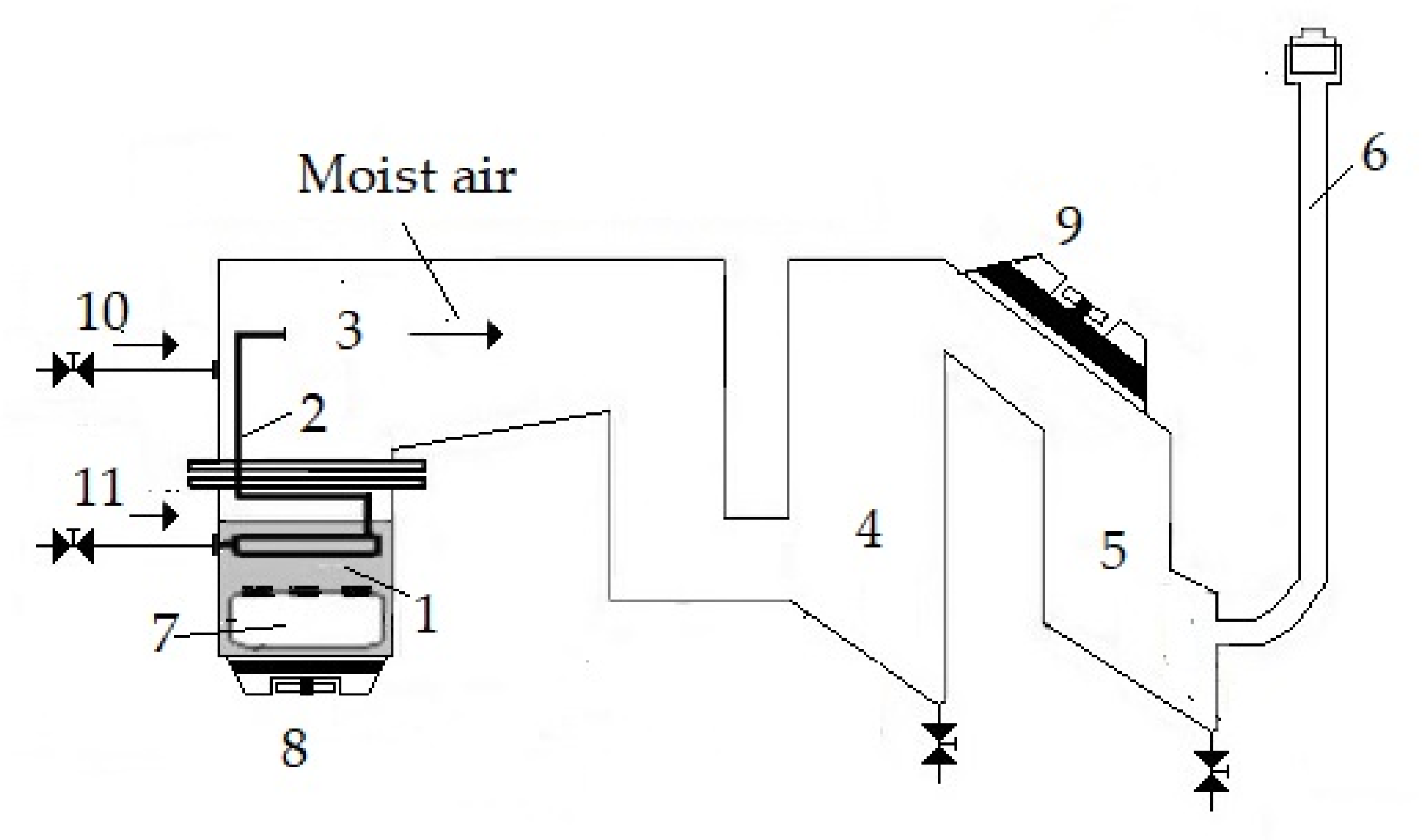
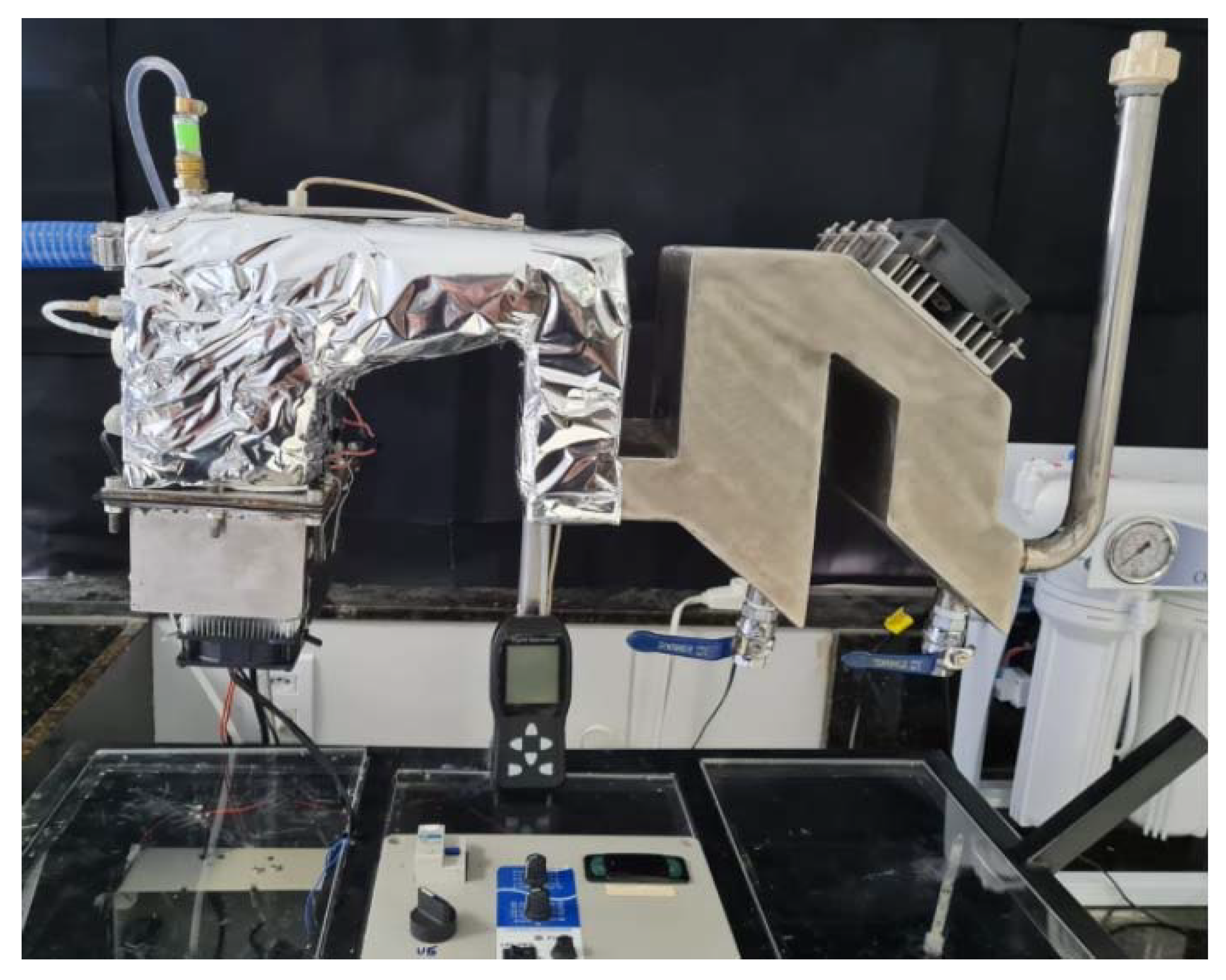
2.1. Experimental Setup

The bench-scale prototype (Figure 1) consisted of an atomization tank (1), a coil for the introduction and heating of atmospheric air (2), a mixing chamber (3), two condensation chambers (4,5), and a duct for the discharge of air (6). A bank of transducers (7) with piezoelectric crystals was installed at the base of the atomization tank to generate ultrasound waves (1.7 MHz). A cooler was installed at the base of the ultrasonic vaporization compartment (8) to help maintain the temperature of the liquid column around 40 °C, as recommended by the manufacturers for the transducers to function properly. Another cooler (9) was installed above the two condensation chambers. Continuous flows of raw water (10) and atmospheric air (11) fed the prototype during the experiments. The atomization tank, with a size of 11 × 16 × 16 cm in length, width, and height, respectively, was equipped with two openings to allow the saline water to enter and the brine to be removed after each test. This prototype was made of 1.5 mm thick AISI 314 stainless steel sheets.

Raw water entered the system at the top of the atomization chamber. To atomize the water, this phase change was accomplished with the aid of the ultrasonic transducers bank [24], consisting of 6 piezoelectric ceramic pellets, with each transducer having a water vaporization capacity of 0.3 kg/h. An internal 0.5 mm copper coil was immersed in the liquid column above the transducer bank. This strategy was used to heat the atmospheric air with the heat released by the water during its atomization, increasing the saturation capacity of the air stream. The final stretch of the coil that was above the free surface of the water column was straightened and carried the flow of hot air to direct the ultrasonic mist to the condensing chambers. A mixture consisting of atomized water and hot air passed through three kinds of compartments. First, it passed through a pre-chamber containing a kind of ramp, which should contribute to the return of raw water due to its possible dragging by an air current under the effect of vortex formation. After passing through the pre-chamber, the heated moist air entered condensing chamber 1, where most of the water carried by the air stream was condensed. At the base of this chamber, a valve allowed the removal of samples for condensate analysis. Most of the remaining atomized water condensed in chamber 2 and was removed by a sampling valve installed at its base. A duct was installed to separate the ultrasound steam and air through a polymer plate installed on the top of this duct. The thickness of the pile formed by polymer plates was responsible, together with the flow of hot air, for the pressure of the system. Two coolers were installed on the condensation chambers to facilitate the collection of the condensed water formed by the ultrasound steam.

Figure 2 shows the bench prototype after construction and installation along with thermal insulation, mounted on a skid adapted for its electrical and electronic accessories.

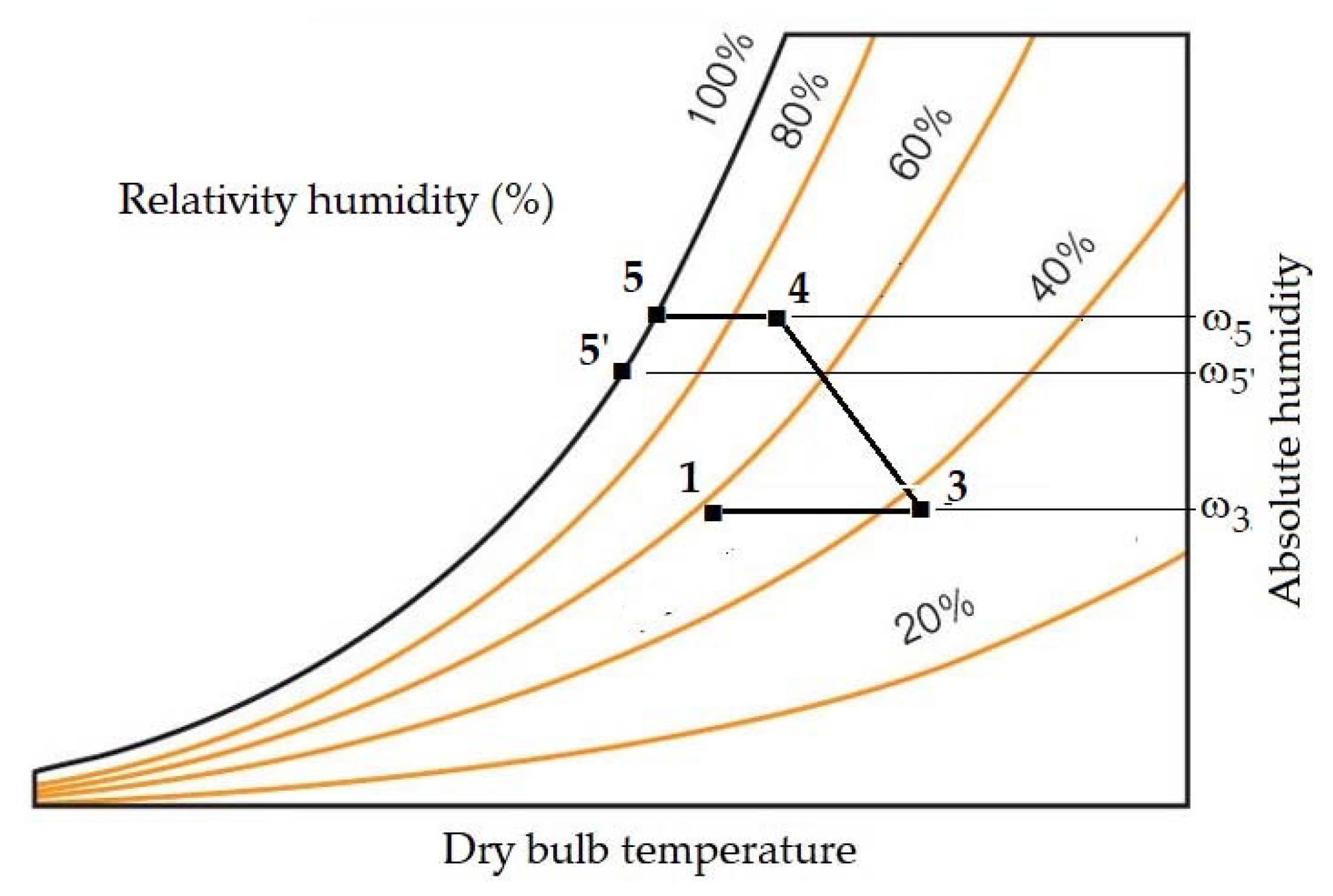
2.2. Analysis of Psychrometric Conditions

The addition of moisture to the air without variation in its dry-bulb temperature is called humidification, while moisture removal without variation of this same temperature is called dehumidification. In industrial practice, these two types of processes are rarely encountered, and humidification/dehumidification processes are usually accompanied by air heating and cooling, respectively [25]. As can be seen in Figure 1, at point 11, the atmospheric air is in psychrometric conditions, illustrated by the psychrometric chart outlined in Figure 3 [26,27]. From point 11 to point 3, a temperature increase occurs due to a heat exchange through the coil immersed in the liquid column. In the region around point 3, the air becomes saturated due to the presence of water vapor formed by ultrasonic atomization. In chambers 4 and 5, the water contained in the air stream condenses and is collected as a product of dehumidification caused by the reduction of dry-bulb and wet-bulb temperatures (5’). From point 5, the air stream is discharged into the atmosphere, passing through the duct, which has at its upper end a pellet of polymeric material that retains a large part of the residual water contained in the air.

Under steady-state conditions, the mass flow rate of dry air (${\dot{m}}_{air}$) entering the bench prototype must be equal to the mass flow rate of dry air unloaded. Thus, according to Figure 3, the maximum mass flow rate of atomized water [28] is equal to that of ultrasonically atomized water, ${\dot{m}}_{wus}$:

$${\dot{m}}_{wus}={\dot{m}}_{air}\left({\omega }_3-{\omega }_2\right)$$

(1)

where:

• ${\dot{m}}_{wus}$—mass flow rate of atomized water, kg of water/s;
• ${\dot{m}}_{air}$—inlet mass flow rate of dry air, kg of dry air/s;
• ${\omega }_2$—absolute humidity at point 2, kg of water/kg of dry air;
• ${\omega }_3$—absolute humidity at point 3, kg of water/kg of dry air.

It is known that a variation in temperature can help to increase the amount of water to be transported by air [29]. It is also known that the volumetric flow rate of air, q_air, which contains the amount of dry air needed to draw this vaporized water, can be estimated as:

$$q_{air}={\dot{m}}_{air}{v}_{air}$$

(2)

where υ_air is the specific volume of air (m³/kg of dry air). Thus, by inserting Equation (1) into Equation (2) and using the expression of the specific volume of air proposed by Wilhelm [30], Equation (3) is obtained:

$$q_{air}=0.2871(t+273.15)(1+1.6078{\omega }_3)\frac{{\dot{m}}_{wus}}{p({\omega }_3-{\omega }_2)}$$

(3)

where:

• t—dry-bulb temperature, °C;
• p—total pressure, kPa.

2.3. Mass and Energy Balances

The water balance in the ultrasonic prototype (Figure 1) can be written as follows [31]:

$${\dot{m}}_{air2}{\omega }_2+{\dot{m}}_{wus}={\dot{m}}_{w4}+{\dot{m}}_{w5}+{\dot{m}}_{air5}{\omega }_5$$

(4)

where:

• ${\dot{m}}_{air2}$—mass flow rate of dry air at point 2, kg/s;
• ${\dot{m}}_{w4}$—mass flow rate of water collected in chamber 4, kg of water/s;
• ${\dot{m}}_{w5}$—mass flow rate of water collected in chamber 5, kg of water/s;
• ${\dot{m}}_{air5}$—mass flow rate of dry air at point 5, kg of dry air/s;
• ${\omega }_5$—absolute humidity at point 5, kg of water/kg of dry air.

The recovery efficiency of treated water by condensation (${\eta }_{cond}$) in the bench prototype is:

$${\eta }_{cond}=\frac{{\dot{m}}_{w4}+{\dot{m}}_{w5}}{{\dot{m}}_{wus}}$$

(5)

As the dry air mass flow rate was the same at the inlet and outlet of the bench-scale prototype, that is, ${\dot{m}}_{air2}={\dot{m}}_{air5}$, Equation (5) can be rewritten, with the aid of Equation (4), as:

$${\eta }_{cond}=\frac{{\dot{m}}_{w4}+{\dot{m}}_{w5}}{{\dot{m}}_{w4}+{\dot{ m}}_{w5 }+{\dot{m}}_{air2 }\left({\omega }_5-{\omega }_2\right)}$$

(6)

An energy balance for the bench-scale prototype, based on Equation (4), taking into account the thermal inertia of water remaining in the liquid phase in the atomization chamber considered as an adiabatic system, can be written as follows [31]:

$${\dot{m}}_{air2}{h}_{air2}+{\dot{m}}_{wus}{h}_{wus}+{\dot{m}}_{wus}{C}_{pw}\left(T_w{-T}_{amb}\right)={\dot{m}}_{w4}{h}_{w4}+{\dot{m}}_{w5}{h}_{w5}+ {\dot{m}}_{air5}{h}_{air5}$$

(7)

where:

• $h_{air2}$—air specific enthalpy of moist air at point 2, kJ/kg;
• $h_{wus}$—specific enthalpy of ultrasonically atomized water, kJ/kg;
• ${\mathrm{C}}_{pw}$—specific heat capacity of water in the liquid phase in the atomization chamber, kJ/(kg·K);
• $T_w$—temperature of the atomization chamber, K;
• $T_{amb}$—ambient temperature, K;
• $h_{w4}$—specific enthalpy of condensed water at point 4, kJ/kg;
• $h_{w5}$—specific enthalpy of condensed water at point 5, kJ/kg;
• $h_{air5}$—specific enthalpy of moist air at point 5, kJ/kg.

Thus, for an accurate assessment of the energy balance in the water ultrasonic treatment prototype, the specific enthalpy of the atomized water was estimated as:

$$h_{wus}=\frac{{\dot{m}}_{w4}{h}_{w4}+{\dot{m}}_{w5}{h}_{w5}+{\dot{m}}_{air2}(h_{air5}-h_{air2})-{\dot{m}}_w{C}_{pw}(T_w-T_{amb})}{{\dot{m}}_{wus}}$$

(8)

The technical specifications of the instrumentation used for experiments are summarized in

Table 1. Technical specifications of the instrumentation used in the experimental setup.

Measuring Instrument	Accuracy	Range
Oscilloscope	$\pm 2\%$	10–300 MHz
Voltmeter	$\pm 0.5\%$	45–260 V
Digital Wattmeter	$\pm 0.7\%$	0.5–22,000 W
Thermohygrometer
Temperature	$\pm 0.5\%$	−20–70 °C
Relativity Humidity	$\pm 1\%$	0–100%
Multi-Digital Camera	$\pm 1.5$ °C	−20 to 400 °C
E-Type Thermocouple	$\pm 1.7\%$	−270–870 °C

.

2.4. Principal Component Analysis (PCA)

The identification of variables that can effectively contribute to the success of equipment can also be used to define the limits of certain operating conditions. Due to the large number of dimensions present in the analysis of this type of system, identifying the process variables that could have a major impact on its performance becomes a complicated task if adequate tools are not used. A recommended solution is the use of statistical techniques of multivariate analysis, more specifically, the Principal Component Analysis (PCA) [32].

PCA is a method of ordering variables, whose results consist in the formation of new axes composed of the combination of descriptor variables and the importance regarding the variability and influence of each one of them on the phenomenon under investigation. The method establishes a set of axes (or factors) perpendicular to each other, in which each component is an eigenvector obtained from the linear correlation matrix or from the covariance matrix, depending on the variables used. The axis length is the eigenvalue of this matrix, which corresponds to the degree of variation of the factor in the experiment. By determining the eigenvectors and eigenvalues of the matrix, a coordinate system is obtained that provides the similarity of samples and their degree of variation in the experiment. The first factor (or axis) of the PCA represents the factor with the highest degree of variance in the data. Interpreting a PCA consists of defining what each axis represents in the sense of the factor. Interpretation become increasingly difficult as its eigenvalue decreases its share of variance [33].

The use of PCA facilitates the identification of components that could best represent the effect of factors on the variability of the system under study. This method allows to reduce the dimensionality of the database while retaining as much of the information present in the data as possible [34]. Generally, more than 80% of the information present in the original variables is obtained in only two or three of the first principal components, in addition to helping to judge the importance of the chosen original variables. In other words, the variables with the greatest weight in the linear combination of the first principal components are the most important from a statistical point of view, allowing to establish correlations among such variables and between them and the variable or set of response variables of interest.

As shown in Equation (9), a principal component (Y_j) is obtained by the linear combination of the values of each measured variable (X_j) [35]:

$$Y_j=a_{i1}{X}_1+a_{i2}{X}_2+\dots +a_{in}{X}_n$$

(9)

multiplied by the coefficients for the j-th factor (a_ij), also called loadings.

When creating scores for the principal components, the loadings of all the original variables are used, some of which, however, are larger, and others close to zero. The solution found to define valid loadings has been to establish a cutoff value. However, if the main component is used only for exploratory data analysis, whether or not these minor values are retained does not matter [35].

The choice of relevant factors for the study of the system must be based on the operating conditions of the system under study. In this case, the following factors were considered important for the use of the ultrasonic treatment system: hot air flow rate (X₁), L/h; raw water conductivity (X₂), μS/cm; carrier air temperature (X₃), K; pressure inside the prototype (X₄), cm H₂O; and percentage efficiency of raw water conductivity reduction (X₅), %.

2.5. Data Collection and Preparation

The first step in collecting data for the application of PCA is to establish the number of samples. This number must be at least equal to the number of variables multiplied by the minimum number of experiments to obtain the sample mean of the variable. The data are then normalized through their means and standard deviations. The sequence of operations for standardization is: (a) calculation of the average of the gross values of each parameter; (b) calculation of the standard deviation of each parameter; and (c) calculation of the standardized value based on Equation (10) [36]:

$$X_i=\frac{x_i-\overline{x}}{s}$$

(10)

where:

• X_i—standardized value;
• x_i—individual observation;
• $\overline{x}$—arithmetic mean;
• S—standard deviation.

At the end of this process, standardized values are obtained with a standard deviation equal to one, for all variables, which is necessary due to the nature and amplitude of the characteristics studied. Thanks to the standardization, the variances of the parameters become comparable among themselves, avoiding that a certain characteristic becomes dominant due to its amplitude or scale.

2.6. Statistical Analysis of Data

Data were submitted to normality (Student’s t) and homogeneity (Cochran) tests. Given these conditions, the aforementioned data were submitted to analysis of variance (ANOVA), followed by Tukey’s test, when necessary, to compare the averages between the results obtained, with a level of significance (p) < 0.05, in case there was no normality and homogeneity of the data. In order to carry out the PCA, it was necessary to decide on the number of components to be retained, that is, how many components were necessary to explain the variability of the data. We opted for the use of the Kaiser’s criterion [37], according to which principal components whose eigenvalues are >1, or that have a variance ≥ 70%, must be retained. To process the analysis, both for descriptive statistics and for principal components, the Statistica Version 12 software (StatSoft, Tulsa, OK, USA) was used.

3. Results and Discussion

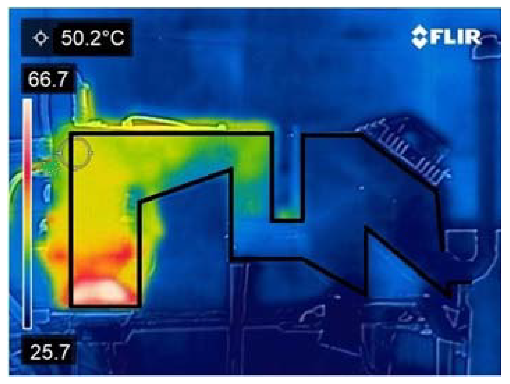
3.1. Bench Prototype Thermal Profile

Figure 4 shows a thermographic image of the ultrasonic treatment prototype, to obtain which we used a FLIR C5 digital camera with a generator of precise thermal images of 160 × 120 (19,200 pixels) (Multi-Spectral Dynamic Imaging, MSX), 5-megapixel visible light, and an LED flashlight. To perform the thermographic recording, the external surfaces of the prototype were coated with black anti-reflective material. In this figure, a temperature of 66.7 °C was recorded as a result of the thermal inertia of the liquid column in the ultrasonic vaporization compartment. A maximum value of 70 °C was obtained for the drag air of the mist formed by the ultrasonic atomization of raw water. This value was presented as a limitation of the heating capacity of this air stream by the thermal inertia of the raw water column in the ultrasonic vaporization chamber.

3.2. Results of Principal Component Analysis

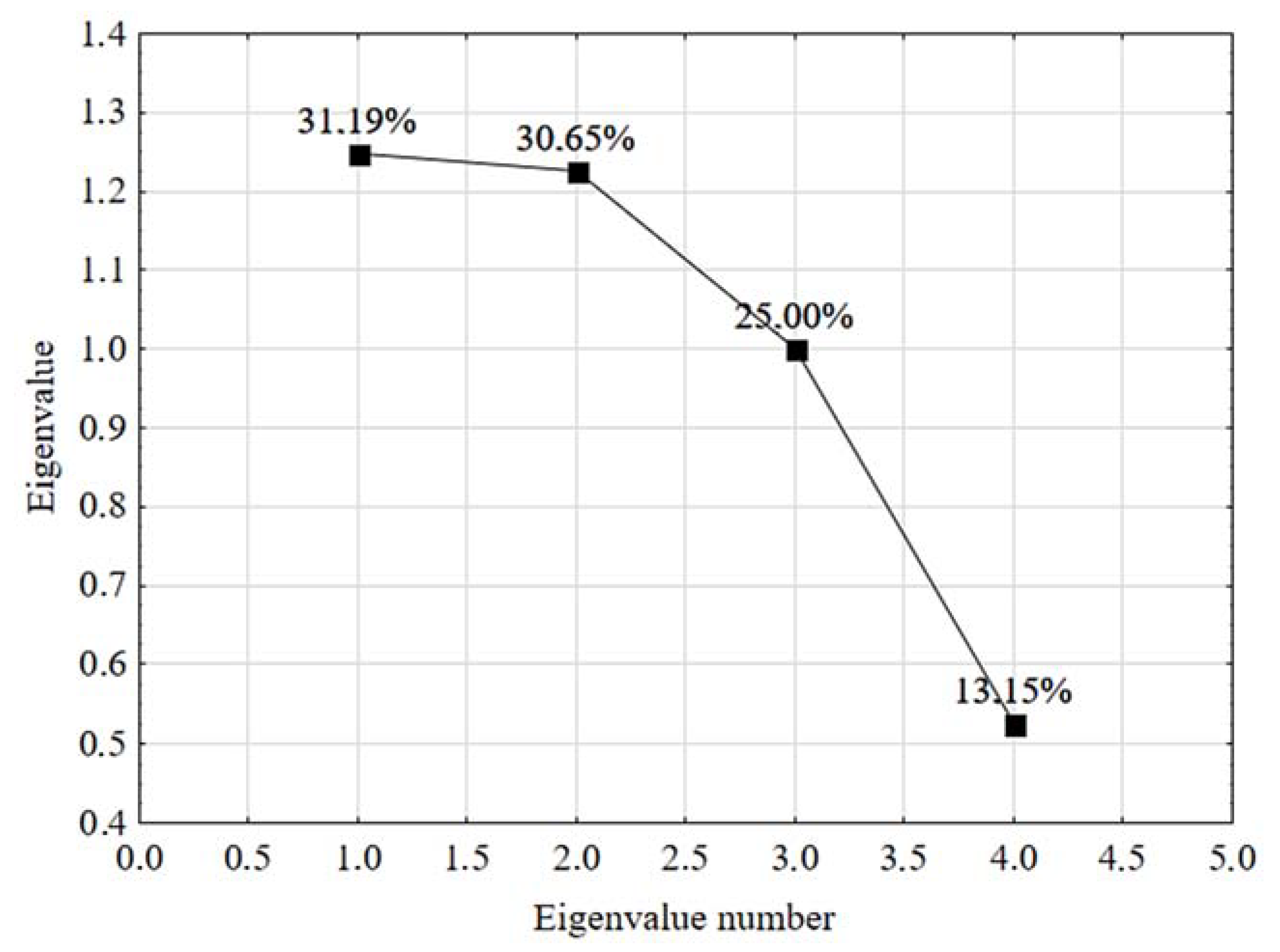
After arrangement in the form of a table, the results of the Principal Component Analysis (PCA) were standardized by Equation (10) and listed in

Table 2. Summary of standardized results of Principal Component Analysis applied to experiments carried out on the bench-scale prototype for boiler water ultrasound treatment.

Run	X1 (L/h)	X2 (μS/cm)	X3 (K)	X4 (cm H2O)	X5 (%)
1	0.000	−0.467	−0.471	−0.438	−0.336
2	2.000	−0.467	−0.471	−0.438	−1.497
3	−2.000	−0.467	−0.471	−0.438	−1.265
4	0.000	0.884	−0.471	−0.438	0.361
5	0.000	2.386	−0.471	−0.438	1.755
6	0.000	−0.467	0.943	−0.438	−0.103
7	0.000	−0.467	2.357	−0.438	0.826
8	0.000	−0.467	−0.471	0.548	−0.103
9	0.000	−0.467	−0.471	2.521	0.361

.

The data in Table 2 were then transferred to the Statistic software, and the appropriate intercorrelation analyses of the original variables were carried out.

3.2.1. Eigenvalue

In a PCA, the eigenvalue measures the percentage of variance explained by each principal component.

Table 3. Eigenvalues, percentage of explained variance, cumulative eigenvalues, and cumulative percentage of explained variance (%) of the principal components.

Principal Component	Eigenvalue	Total Variance (%)	Cumulative Eigenvalue	Cumulative Total Variance (%)
1	1.247791	31.19477	1.247791	31.1948
2	1.226021	30.65052	2.473812	61.8453
3	1.000000	25.00000	3.473812	86.8453
4	0.526188	13.15471	4.000000	100.0000

records, for each principal component, the respective eigenvalues, the percentage of explained variance, the cumulative eigenvalues, and the cumulative percentage of explained variance. These data were used to select the number of principal components responsible for capturing most of the variation in the data. In this analysis, the minimum number of required principal components was three, being responsible for explaining no less than 86.84% of the variance of the four original variables.

3.2.2. Scree Plot Graph

The data listed in Table 3 were used to create a scree plot graph (Figure 5), where the percentage of explained variance of the principal components is illustrated in descending order. An abrupt slope reduction is normally expected as a criterion for retaining or excluding a number of major components. In this case, the criterion of eigenvalue equal to or above the mean value one was sufficient to retain the first three principal components.

3.2.3. Statistical Importance of Variables

The eigenvectors represent the principal components and result from the assignment of coefficients to each of the original variables (loadings). Such loadings can be considered as a relative measure of the importance of each variable in relation to the principal components, and the signs, positive or negative, of the loadings indicate directly or inversely proportional relationships.

Table 4. Characteristic loading coefficients for the first three principal components.

	PC1	PC2	PC3
X1	0.000000	0.000000	1.000000
X2	−0.763880	0.488767	0.000000
X3	0.813313	0.399881	0.000000
X4	−0.052919	−0.909518	0.000000

summarizes the loadings corresponding to the eigenvalues retained in this PCA applied to the bench-scale prototype used in this work.

The first principal component (PC₁) was a new variable, Y₁, whose value for each observation was given by the equation [35]:

$$Y_1=-0.763880X_2+0.813313X_3-0.052919X_4$$

(11)

that explained 31.19% of the total variance in the data. In addition, this first eigenvalue that was determined corresponded to the highest percentage of total variability present, and so on with the others. This first major component retained contributions from raw water conductivity (X₂) and carrier air temperature (X₃). These variables exhibited loadings above 0.7 and were practically responsible for the way in which this new variable had the total variance with the highest value. In the case of X₂, the loading had a negative sign, i.e., inverse proportionality to this new variable. A high salt concentration in the raw water leads to a high concentration of these salts in the treated water. A loading with a positive sign was observed for the temperature of the carrier air (X₃), indicating a direct proportionality. Positive variations in temperature were responsible for a considerable capacity of carrier air to retain ultrasonic steam, resulting in a greater amount of treated water.

The behaviors observed for variables X₂ and X₃ agreed with the observations of Hosseingholilou et al. [19].

In the linear combination that gave rise to the PC2 (Y₂), we obtained:

$$Y_2=0.488767X_2+0.399881X_3-0.909518X_4$$

(12)

In this main component, which explained 30.65% of the total variation of the data, it was observed that the prototype internal pressure (X₄) was responsible for most of this contribution. The negative sign of the X₄ loading can be explained by the increasing difficulty of ultrasonic vaporization of raw water with increasing pressure. Despite the high absolute value of this loading, its presence in the second principal component reduced its importance in explaining the phenomenon compared to variables X₂ and X₃, which were the dominant ones in Y₁.

The principal component 3 (PC3), or Y₃, which explained 25.0% of the variation in the data, had only the carrier air flow rate (X₁) as a constituent:

$$Y_3=1.000000X_1$$

(13)

However, this original variable appeared to be dependent on the others, since to contribute to the increase in the efficiency of the treatment of feed water, this effect is dependent on its own temperature, the concentration of impurities in the water, and the ambient pressure.

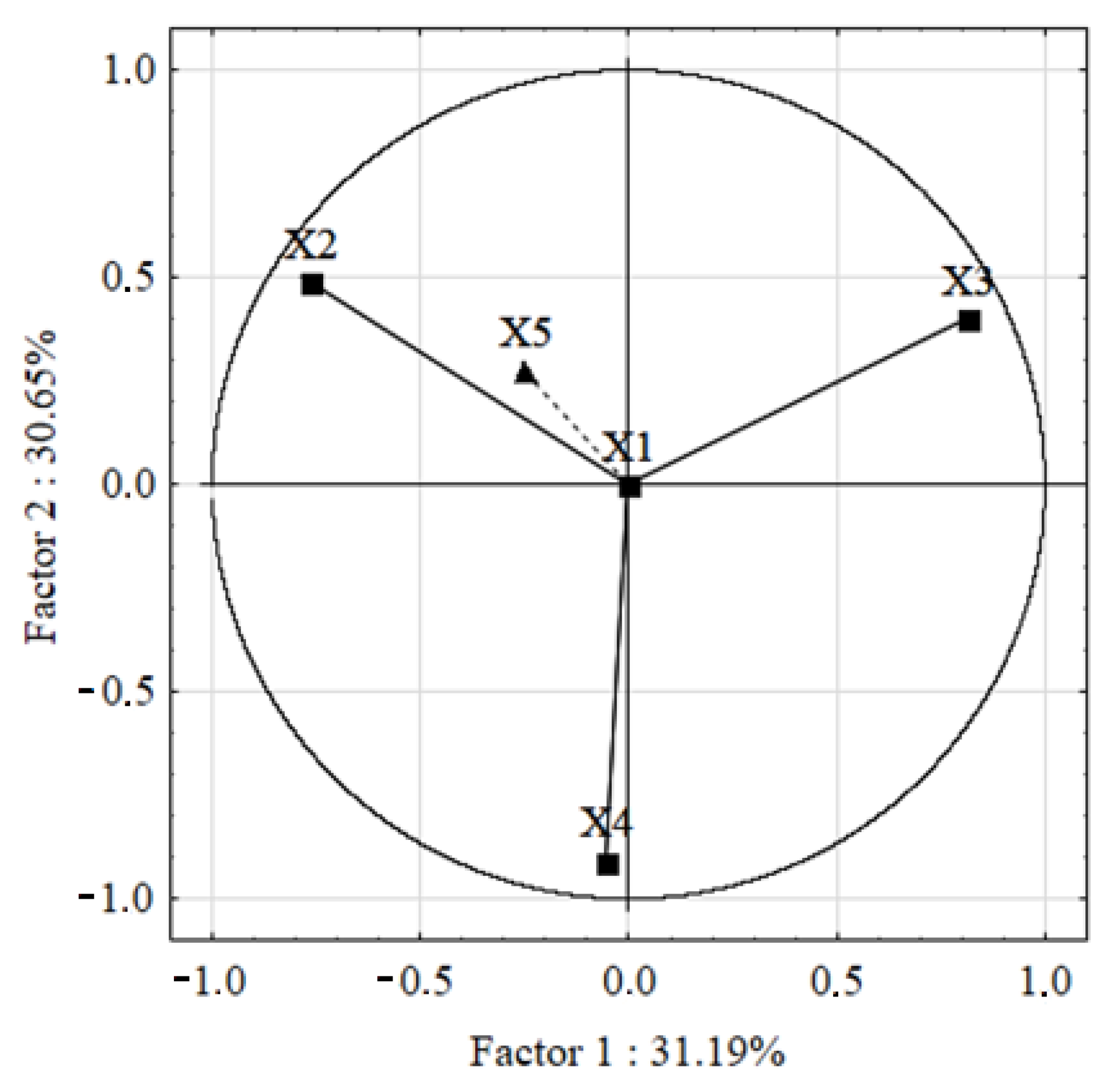
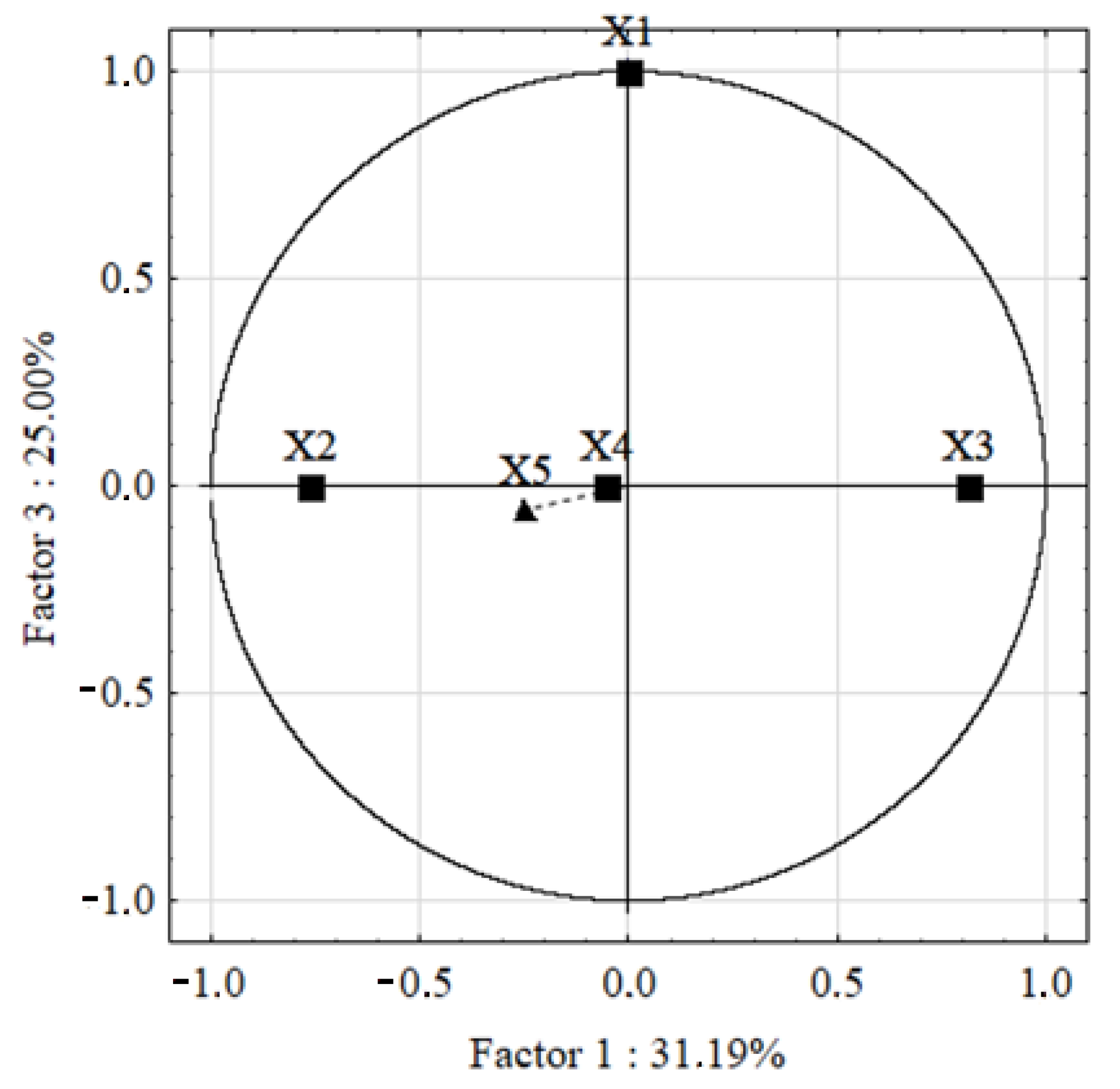
3.2.4. Hypersphere Graphs and Loading of Variables

Variables X₂ and X₃ were the most important variables for PC1, as can be seen in Figure 6 by the projections of the loadings on the PC1 axis, compared to the other variables. The greater the contribution of a variable, the wider the projection. It can also be seen that such variables have different effects depending on the opening of the angle between them. The signs assigned to the semi-axes of their projections also demonstrate these characteristics. As for the treatment efficiency (X₅), X₂ has the same sign and, therefore, is directly proportional to it, whereas the opposite occurs for X₃. When observing the projections of the variable loadings on PC2, the prototype internal pressure (X₄), with a negative sign, has the greatest projection compared to the others.

Figure 7 allows a very simple analysis between PC1 and PC3, with the latter being fully represented by the loading of the carrier air flow (X₁). Regarding the variable X₅, the variable X₁ has inverse proportionality.

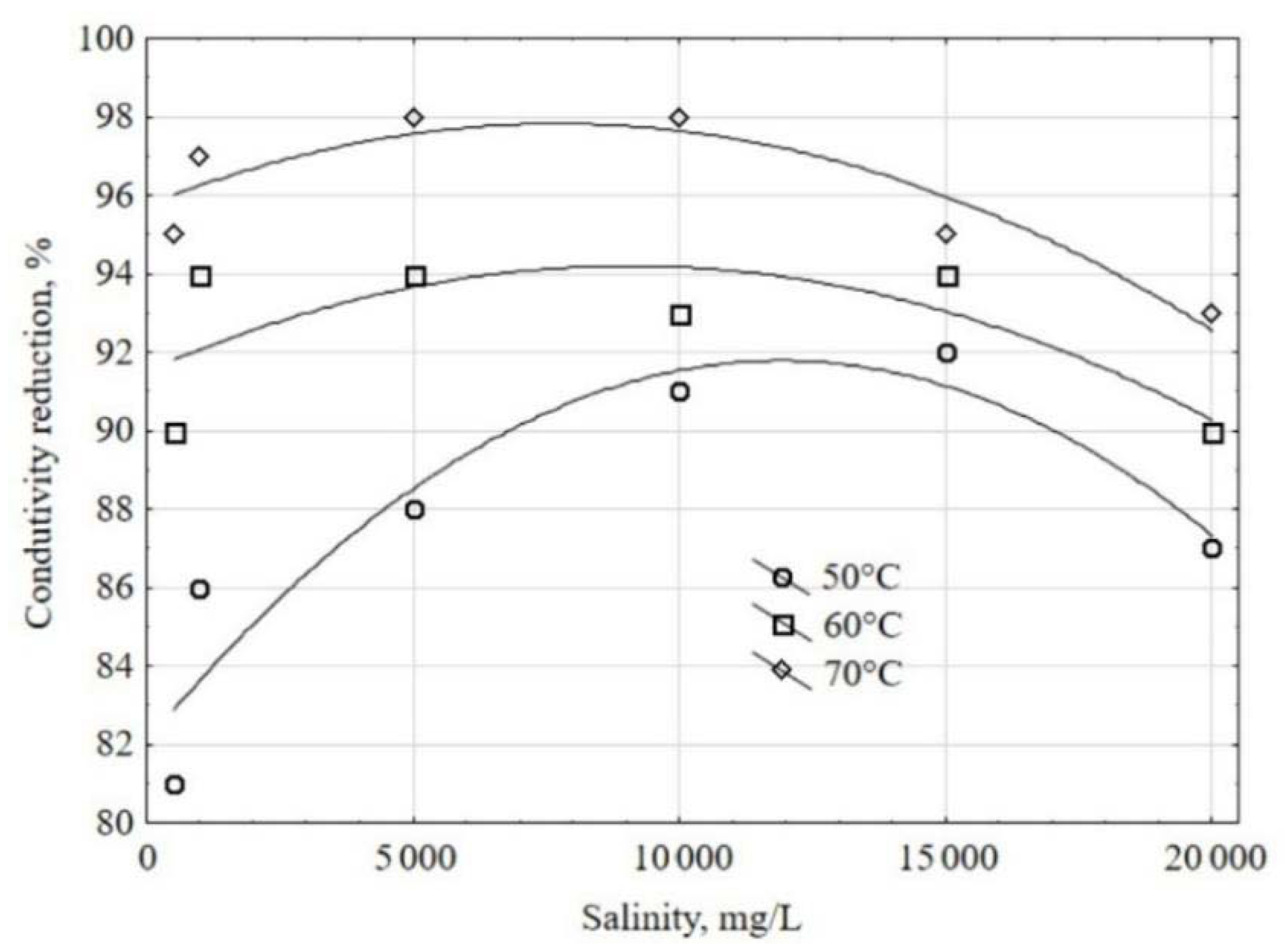
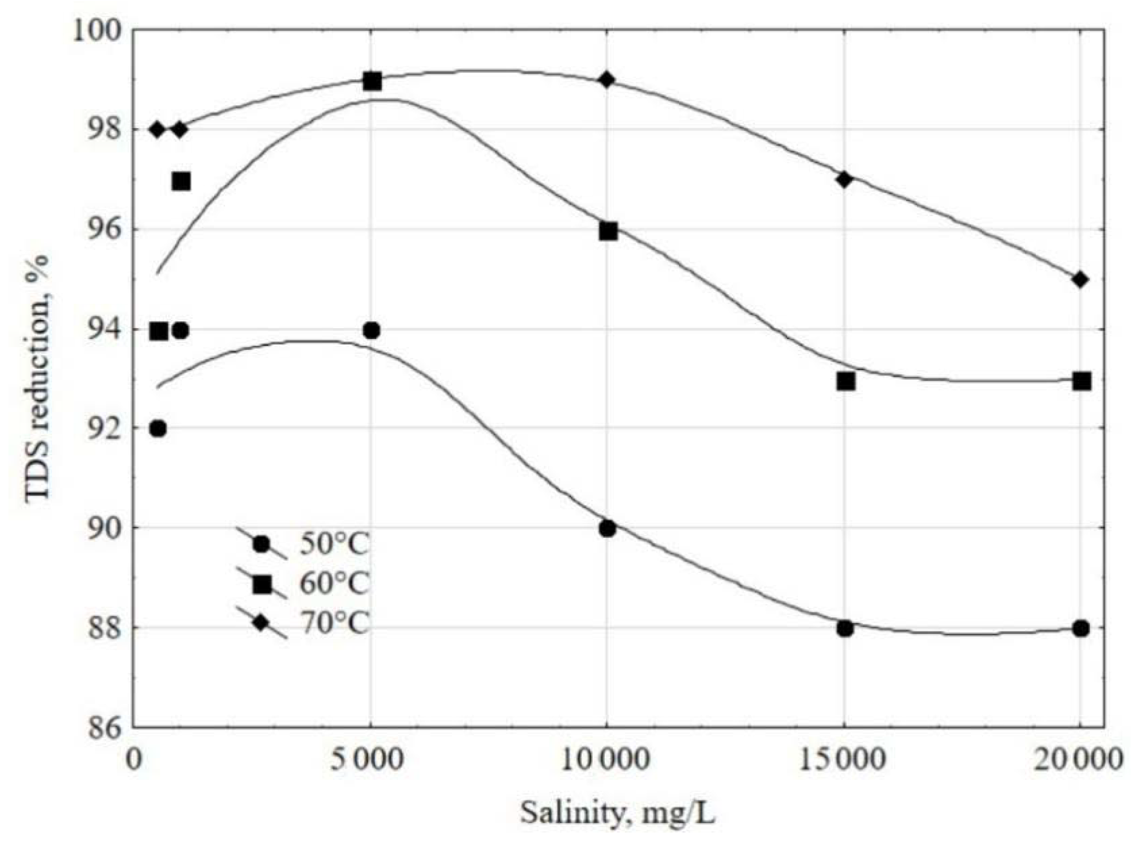
3.3. Tests with Feed Waters with Different Salinities

The use of treated water by operators of industrial boiler installations has been recurrent. However, such facilities need to be prepared for unforeseen events and the use of water with salinity above 500 mg/L. Collections of moderately brackish water with salinity of up to 20,000 mg/L were performed, and salinity adjustments (5000, 10,000, 15,000, and 20,000 mg/L) were made to carry out experiments with the ultrasonic bench-scale prototype. Figure 8 illustrates the results obtained for reductions in the conductivity of the feed water at different temperatures of the air mixed with the ultrasonic steam, maintaining an ultrasonic steam mass flow rate of 3 kg/h and an air mass flow rate of 25 kg/h, or a ratio between the mass flow rates of water and air in the order of 0.0045 [17]. For low salinity values, an increase in temperature causes an increase in moisture retention by the air and, consequently, an increase in the efficiency in reducing conductivity. Subsequently, an increase in the feed water salinity is reflected in an increase in the residual salinity of the treated water, in line with the observations taken from the PCA results. Therefore, the behavior of the percentage reduction in the conductivity of the treated (condensed) water showed a slight reduction as the salt concentration in the feed water increased. To confirm these observations, a graph of the percentage reduction of total dissolved solids was made (Figure 9), whose behavior, as predicted, followed what was observed for the percentage reduction in conductivity.

Water vaporization is a process in which high-energy molecules meet on the free surface of the liquid column and are easily transported to the vapor phase [38]. In this phase change, a considerable amount of heat is lost to the non-vaporized part [39,40]. The heating time of the lower range of the water column presents a considerable delay in the temperature increase due to its high thermal inertia. On the other hand, the vaporization velocity at the surface has a small thermal inertia and responds very quickly to temperature variation, culminating in a considerable reduction in energy consumption for steam production. In the case of ultrasonic vaporization, caused by high-frequency waves [41] in the ultrasonic vaporization chamber of the bench-scale prototype, the liquid bed was heated and, due to this large thermal inertia, a considerable amount of heat was left in this bed. Thus, the energy retained by the ultrasonic vaporization chamber was used to heat the carrier air.

In evaluating the performance of the ultrasonic prototype for boiler water treatment per unit of energy consumed, the specific productivity was used, that is, the amount of treated water produced per unit of energy. The calculations used to make Figure 10 took into account the specific enthalpy of water vaporized ultrasonically (336.92 kJ/kg) estimated by Equation (8). This value was 16.5% higher than the enthalpy of water in the saturated liquid state at 303 K. The specific productivity was higher than those obtained by Tourab et al. [17] and Hosseingholiliou et al. [19]. Such discrepancy can be justified by the use of energy made available by the thermal inertia of the vaporization chamber and by the use of a simpler and more economical refrigeration system.

After confirming the responses of the bench-scale prototype for water of different salinities, experiments were carried out to verify the conditions of compliance with the analysis specifications of the TERMOCABO boiler (

Table 5. Values of physicochemical parameters for water and treated water before and after a single pass through the irradiation chamber of the bench-scale prototype.

Control Parameter	Recommended Value for the Pressure Range of 10–20 kgf/cm2	Experimental Results
		Raw Water	Treated Water
pH	10.5–11.5	8.49 ± 0.05	7.75 ± 0.01
Conductivity (μS/cm)	<4000	616 ± 6	59.60 ± 0.04
Alkalinity (mg/L CaCO3)	<800	80 ± 1	15.00 ± 0.01
Alkalinity as NaOH (mg/L CaCO3)	150–350	-	-
Chloride (mg/L Cl)	<400	130 ± 2	15.00 ± 0.01
Total hardness (mg/L CaCO3)	<2.0	135 ± 2	1.00 ± 0.01
Total iron (mg/L Fe)	<5.0	-	-
Phosphate (mg/L PO43−)	30–50	6.21 ± 0.01	1.61 ± 0.01
Sulphite (mg/L SO32−)	30–50	5.00 ± 0.01	10.00 ± 0.01
Silica (mg/L Si)	<150	-	-
Total dissolved solids (mg/L)	<300	273 ± 3	35.28 ± 0.02

):

• Mass air flow rate: 25 kg/h;
• Air temperature at the mixing point with atomized water: 70 °C;
• Feed water conductivity: 5000 μS/cm;
• Pressure inside the prototype: 18 cm H₂O.

4. Conclusions

The novelty of this study was the development of a bench-scale prototype of a boiler water treatment system equipped with water atomization by ultrasonic (US) vibrations able to operate at pressures just above the atmospheric one and a maximum temperature of 70 °C, which would allow the use of low-cost material in case of scaling up. This maximum temperature was presented as a limitation of the heating capacity of the carrier air, using only the thermal inertia of the proposed process. Using the Principal Component Analysis multivariate statistical tool, the analysis of the contributions of the variables relevant to the desalination process became more productive, fast, objective, and efficient. The results suggest that the US technique may be an interesting option for water desalination. Its main advantages over reverse osmosis are a very low volume of tailings (about 2% per passage), the lack of a raw water pre-treatment step, and the use of energy provided by thermal inertia stored in the liquid phase during the acoustic atomization stage, thus increasing the productivity of the desalination process. Future studies are needed to confirm an economically viable number of stages for different ranges of raw water salinity in the feeding of boilers for different steam production capacities.

References

1. Larsen, M.A.D.; Petrovic, S.; Engström, R.E.; Drews, M.; Liersch, M.; Karlsson, K.B.; Howells, M. Challenges of data availability: Analysing the water-energy nexus in electricity Generation. Energy Strategy Rev. 2019, 26, 100426. [Google Scholar] [CrossRef]
2. Martínez Moya, S.; Boluda Botella, N. Review of techniques to reduce and prevent carbonate scale. Prospecting in water treatment by magnetism and electromagnetism. Water 2021, 13, 2365. [Google Scholar] [CrossRef]
3. Zhu, Z.; Rao, R.; Zhao, Z.; Chen, J.; Jiang, W.; Bi, F.; Yang, Y.; Zhang, X. Research progress on removal of phthalates pollutants from environment. J. Mol. Liq. 2022, 355, 118930. [Google Scholar] [CrossRef]
4. Gong, Y.; Wang, Y.; Lin, N.; Wang, R.; Wang, M.; Zhang, X. Iron-based materials for simultaneous removal of heavy metal(loid)s and emerging organic contaminants from the aquatic environment: Recent advances and perspectives. Environ. Pollut. 2022, 299, 118871. [Google Scholar] [CrossRef]
5. Li, X.; Jie, B.; Lin, X.; Deng, Z.; Qian, J.; Yang, Y.; Zhang, X. Application of sulfate radicals-based advanced oxidation technology in degradation of trace organic contaminants (TrOCs): Recent advances and prospects. J. Environ. Manag. 2022, 308, 114664. [Google Scholar] [CrossRef]
6. Čuda, P.; Pospíšil, P.; Tenglerová, J. Reverse osmosis in water treatment for boilers. Desalination 2006, 198, 41–46. [Google Scholar] [CrossRef]
7. Asadi, N.; Soleimanimehr, H.; Alinia-ziazi, A. An investigation on boiler feed water treatment using reverse osmosis and ion exchange by WAVE software. J. Appl. Res. Water Wastewater 2021, 8, 124–128. [Google Scholar] [CrossRef]
8. Fetyan, N.A.H.; Attia, T.M.S. Water purification using ultrasound waves: Application and challenges. Arab. J. Basic Appl. Sci. 2020, 27, 194–207. [Google Scholar] [CrossRef]
9. Chong, M.N.; Jin, B.; Chow, C.W.K.; Saint, C. Recent developments in photocatalytic water treatment technology: A review. Water Res. 2010, 44, 2997–3027. [Google Scholar] [CrossRef]
10. Wang, Z.H.; Liu, X.-Y.; Zhang, H.-Q.; Wang, Y.; Xu, Y.-F.; Peng, B.-L.; Liu, Y. Modeling of kinetic characteristics of alkaline-surfactant-polymer-strengthened foams decay under ultrasonic standing wave. Pet. Sci. 2022, in press. [CrossRef]
11. Huggi, M.; Mise, S.R. Optimized ANN model for ultrasonication wastewater treatment process. Int. J. Adv. Res. Eng. Technol. 2019, 10, 94–102. [Google Scholar] [CrossRef]
12. Stefan, A.; Balan, G. The chemistry of the raw water treated by air-jet ultrasound generator. Rom. J. Tech. Sci. Appl. Mech. 2011, 56, 85–92. [Google Scholar]
13. Leong, T.; Juliano, P.; Knoerzer, K. Advances in ultrasonic and megasonic processing of foods. Food Eng. Rev. 2017, 9, 237–256. [Google Scholar] [CrossRef]
14. Chu, C.-L.; Lu, T.-Y.; Fuh, Y.-K. The suitability of ultrasonic and megasonic cleaning of nanoscale patterns in ammonia hydroxide solutions for particle removal and feature damage. Semicond. Sci. Technol. 2020, 35, 45001. [Google Scholar] [CrossRef]
15. Entezari, M.H.; Tahmasbi, M. Water softening by combination of ultrasound and ion Exchange. Ultrason. Sonochem. 2009, 16, 356–360. [Google Scholar] [CrossRef]
16. Hiratsuka, A.; Pathak, D. Application of ultrasonic waves for the improvement of water treatment. J. Water Resour. Prot. 2013, 5, 604–610. [Google Scholar] [CrossRef] [Green Version]
17. Tourab, A.E.; Blanco-Marigorta, A.M.; Elharidi, A.M.; Suárez-López, M.J. A novel humidification technique used in water desalination systems based on the humidification–dehumidification process: Experimentally and theoretically. Water 2020, 12, 2264. [Google Scholar] [CrossRef]
18. El-Maghlany, W.M.; Tourab, A.E.; Hegazy, A.H.; Teamah, M.A.; Hanafy, A.A. Experimental study on productivity intensification of HDH desalination unit utilizing two-stage dehumidification. Desalin. Water Treat. 2018, 107, 28–40. [Google Scholar] [CrossRef]
19. Hosseingholilou, B.; Banakar, A.; Mostafaei, M. Design and evaluation of a novel ultrasonic desalination system by response surface methodology. Desalin. Water Treat. 2019, 164, 263–275. [Google Scholar] [CrossRef]
20. Niam, A.G.; Sucahyo, L. Ultrasonic atomizer application for Low Cost Aeroponic Chambers (LCAC): A review. IOP Conf. Ser. Earth Environ. Sci. 2020, 542, 12034. [Google Scholar] [CrossRef]
21. Odu, S.O.; Van Der Ham, A.G.J.; Metz, S.; Kersten, S.R.A. Design of a process for supercritical water desalination with zero liquid discharge. Ind. Eng. Chem. Res. 2015, 54, 5527–5535. [Google Scholar] [CrossRef]
22. Choong, W.H.; Nasip, M.N.B. Ultrasonic atomiser system performance characterisation study for water purification system development. Trans. Sci. Technol. 2021, 8, 239–244. [Google Scholar]
23. Van Wyk, S.; van der Ham, A.G.J.; Kersten, S.R.A. Potential of supercritical water desalination (SCWD) as zero liquid discharge (ZLD) technology. Desalination 2020, 495, 114593. [Google Scholar] [CrossRef]
24. Abdelaziz, G.B.; El-Said, E.M.S.; Dahab, M.A.; Omara, M.A.; Sharshir, S.W. Hybrid solar desalination systems review. Energy Sources A Recovery Util. Environ. Eff. 2021, 1–31. [Google Scholar] [CrossRef]
25. Giwa, A.; Akther, N.; Al Housani, A.; Haris, S.; Hasan, S.W. Recent advances in humidification dehumidification (HDH) desalination processes: Improved designs and productivity. Renew. Sustain. Energy Rev. 2016, 57, 929–944. [Google Scholar] [CrossRef]
26. Beltrán-Prieto, J.C.; Beltrán-Prieto, L.A. Estimation of psychrometric parameters of vapor water mixtures in air. Appl. Eng. Educ. 2016, 24, 39–43. [Google Scholar] [CrossRef]
27. Devres, Y.O. Psychrometric properties of humid air: Calculation procedures. Appl. Energy. 1994, 48, 1–18. [Google Scholar] [CrossRef]
28. Garg, K.; Das, S.K.; Tyagi, H. Thermal design of a humidification-dehumidification desalination cycle consisting of packed-bed humidifier and finned-tube dehumidifier. Int. J. Heat Mass Transf. 2022, 183, 122153. [Google Scholar] [CrossRef]
29. Kabeel, A.E.; Hamed, M.H.; Omara, Z.M.; Sharshir, S.W. Water desalination using a humidification-dehumidification technique—A detailed review. Nat. Resour. 2013, 4, 286–305. [Google Scholar] [CrossRef] [Green Version]
30. Wilhelm, L.R. Numerical calculation of psychrometric properties in SI units. Trans. ASAE 1976, 19, 318–321. [Google Scholar] [CrossRef]
31. Chen, Q.; Akhtar, F.H.; Burhan, M.; Kumja, M.; Ng, K.C. A novel zero-liquid discharge desalination system based on the humidification-dehumidification process: A preliminary study. Water Res. 2021, 207, 117794. [Google Scholar] [CrossRef]
32. Groenewald, J.W.D.; Nelson, L.R.; Hundermark, R.J.; Phage, K.; Sakaran, R.L.; van Rooyen, Q.; Cizek, A. Furnace integrity monitoring using principal component analysis: An industrial case study. J. S. Afr. Inst. Min. Metal. 2018, 118, 345–352. [Google Scholar] [CrossRef] [Green Version]
33. Teng, S.Y.; How, B.S.; Leong, W.D.; Teoh, J.H.; Siang Cheah, A.C.; Motavasel, Z.; Lam, H.L. Principal component analysis-aided statistical process optimisation (PASPO) for process improvement in industrial refineries. J. Clean. Prod. 2019, 225, 359–375. [Google Scholar] [CrossRef] [Green Version]
34. Jolliffe, I.T.; Cadima, J. Principal component analysis: A review and recent developments. Phil. Trans. R. Soc. A 2016, 374, 20150202. [Google Scholar] [CrossRef]
35. Bro, R.; Smilde, A.K. Principal component analysis. Anal. Methods 2014, 6, 2812–2831. [Google Scholar] [CrossRef] [Green Version]
36. Husson, F.; Lê, S.; Pagès, J. Exploratory Multivariate Analysis by Example Using R, 2nd ed.; Chapman; Hall/CRC: Boca Raton, FL, USA, 2017; Available online: http://factominer.free.fr/bookV2/index.html (accessed on 17 July 2021).
37. Kaiser, H.F. The application of electronic computers to factor analysis. Educ. Psychol. Meas. 1960, 20, 141–151. [Google Scholar] [CrossRef]
38. Ahmadvand, S.; Abbasi, B.; Azarfar, B.; Elhashimi, M.; Zhang, X.; Abbasi, B. Looking beyond energy efficiency: An applied review of water desalination technologies and an introduction to capillary-driven desalination. Water 2019, 11, 696. [Google Scholar] [CrossRef] [Green Version]
39. Yang, Z.; Lian, Z.; Tao, R.; Zhong, H.K. Experimental study on the performance of the internally-heated ultrasonic atomization liquid desiccant regeneration system. Appl. Therm. Eng. 2019, 163, 114211. [Google Scholar] [CrossRef]
40. Kashyap, V.; Al-Bayati, A.; Sajadi, S.M.; Irajizad, P.; Wang, S.H.; Ghasemi, H. A flexible anti-clogging graphite film for scalable solar desalination by heat localization. J. Mater. Chem. A 2017, 5, 15227–15234. [Google Scholar] [CrossRef]
41. Zhang, X.; Kan, W.; Jiang, H.; Chen, Y.; Cheng, T.; Jiang, H.; Hu, X. Capillary-driven low grade heat desalination. Desalination 2017, 410, 10–18. [Google Scholar] [CrossRef]
Figure 1. Schematic diagram of the bench-scale prototype used to perform boiler water treatment tests with high-frequency ultrasound waves: 1—Atomization tank; 2—Air heating coil; 3—Mixing chamber; 4,5—Condensation chambers; 6—Duct for the discharge of air; 7—Bank of transducers; 8,9—Coolers; 10—Raw water entrance; 11—Atmospheric air entrance.
Energies 15 04431 g001
Figure 2. Bench-scale prototype developed for ultrasonic treatment of boiler water.
Energies 15 04431 g002
Figure 3. Sketch of a psychrometric chart showing the absolute humidity of the points corresponding to those illustrated in Figure 1.
Energies 15 04431 g003
Figure 4. Thermographic profile of the bench-scale ultrasonic prototype for boiler feed water treatment.
Energies 15 04431 g004
Figure 5. Scree plot graph of the percentage of explained variance of the main components for the efficiency of the water ultrasound treatment using the bench-scale prototype.
Energies 15 04431 g005
Figure 6. Biplot graph with projections of the loadings of the main components PC1 and PC2.
Energies 15 04431 g006
Figure 7. Biplot graph with projections of the loadings of the main components PC1 and PC3.
Energies 15 04431 g007
Figure 8. Percentage reduction in conductivity of treated water as a function of the salinity of feed water of the bench-scale ultrasonic prototype for boiler water treatment.
Energies 15 04431 g008
Figure 9. Percentage reduction of total dissolved solids (TDS) in treated water as a function of the salinity of the feed water of the bench-scale ultrasonic prototype for boiler water treatment.
Energies 15 04431 g009
Figure 10. Specific productivity as a function of liquid (L) and gas (G) mass flow rate ratio.
Energies 15 04431 g010