
Review on Interpretable Machine Learning in Smart Grid


Abstract
:1. Introduction
2. Description of Interpretable Machine Learning
2.1. Definition
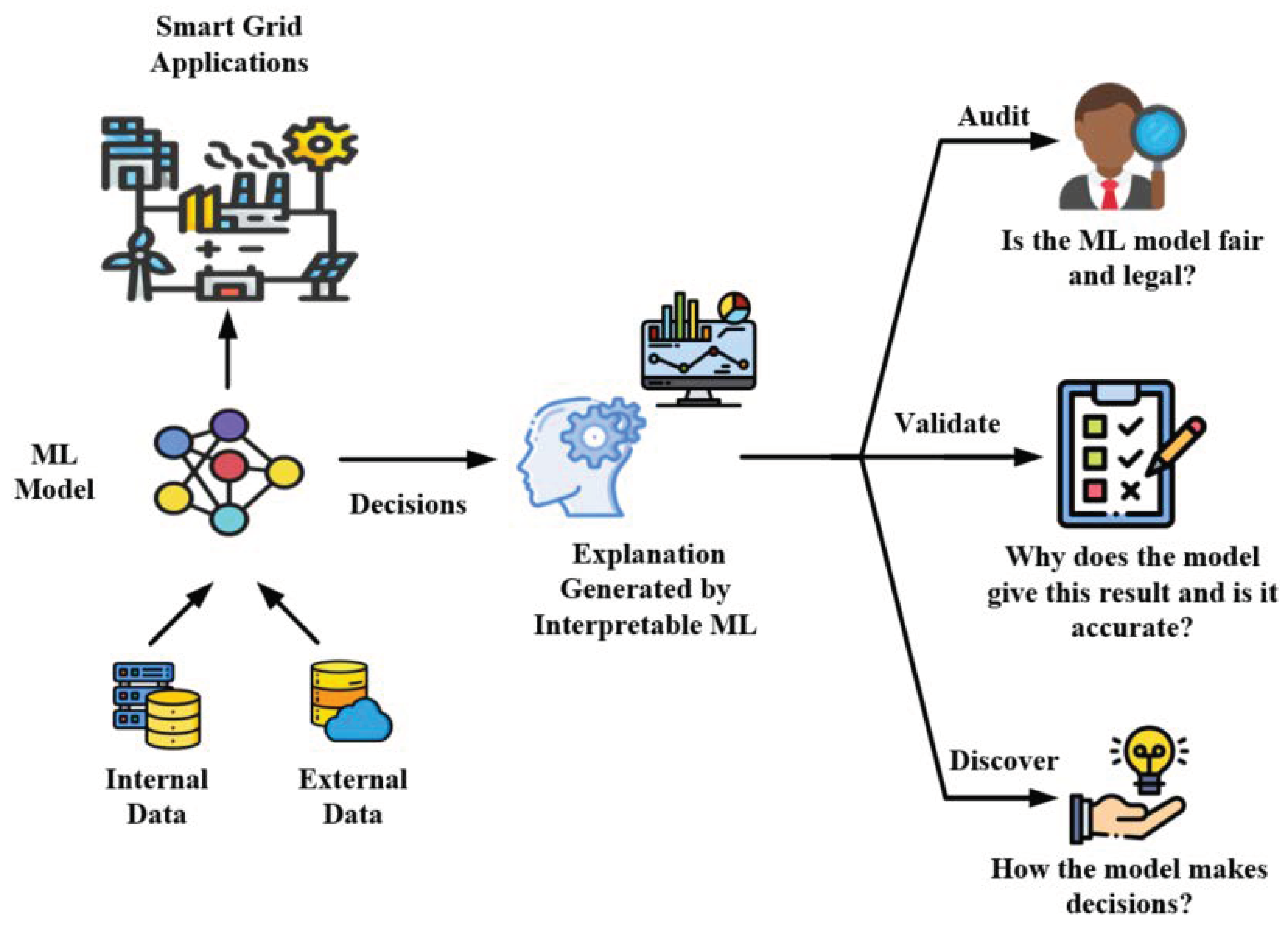
2.2. Motivations
2.2.1. To Audit
2.2.2. To Validate
2.2.3. Discovery
2.3. Properties
- Expressive Power: The language or structure of explanation. Such as logic rules, linear models, statistics, natural language, etc.
- Translucency: Translucency describes how much the explanation method looks inside the ML model. For example, interpretable methods that rely on intrinsically interpretable models are highly translucent. Explanation methods that rely only on inputs and outputs and treat the model as a black box have zero translucency.
- Portability: Portability describes the range of ML models that can be interpreted using this method. Model-agnostic methods are more portable.
- Algorithmic Complexity: The computational complexity of the interpretable methods.
- Accuracy: The ability of an explanation for a decision to generalize to other unseen situations.
- Fidelity: The degree to which the explanation reflects the decision-making behavior of the model. Some explanations only provide local fidelity, such as LIME.
- Consistency: Consistency measures the degree to which models trained on the same task and producing similar predictions produce similar explanations.
- Stability: Stability is the similarity of explanations between similar instances. This criterion targets explanations generated from the same prediction model.
- Comprehensibility: The readability of the explanation (subjective) and the size of the explanation (such as the depth of the DT, the number of weights in the linear model, etc.).
- Certainty: Whether the explanation reflects the confidence of the predicted result.
- Degree of Importance: Does the explanation include the importance of its return component?
- Novelty: Does the explanation reflect that the instance to be explained comes from a new region far from the distribution of the training data? With high novelty, model decisions may be inaccurate.
- Representativeness: Representativeness is the extent to which the explanation can cover the instance. For example, the rule interpretation of a DT can cover the entire model, and the Shapely value only represents the interpretation of a single prediction.
3. Taxonomy of Interpretable Machine Learning
3.1. Pre-Model
3.2. In-Model
3.2.1. Simple Intrinsically Interpretable Models
3.2.2. Self-Explanatory Neural Networks
3.3. Post-Model
3.3.1. Interpretation of Model
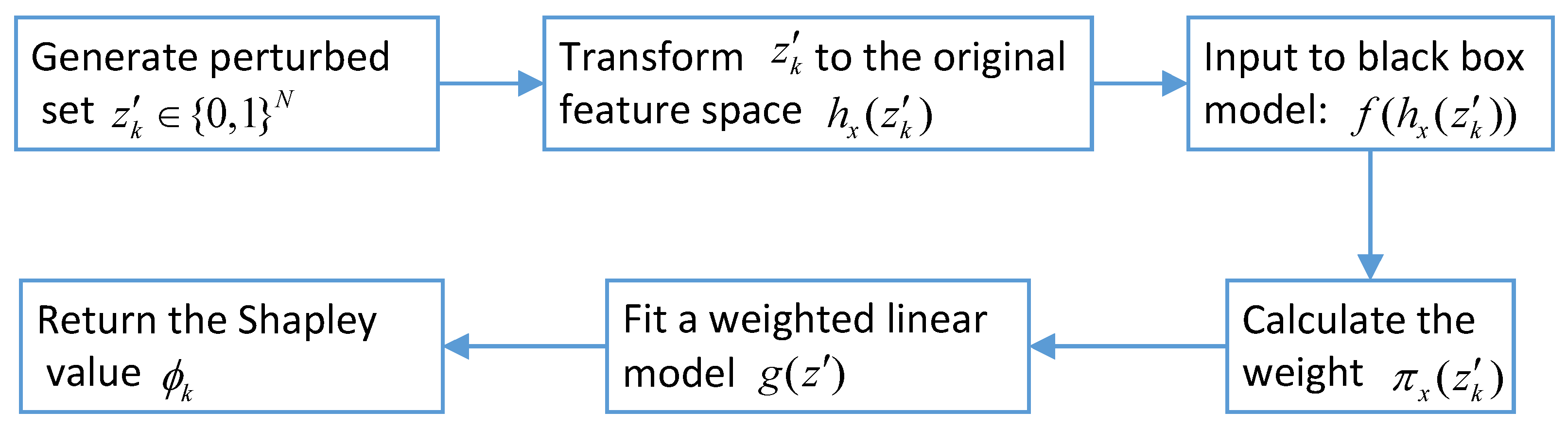
3.3.2. Interpretation of Prediction
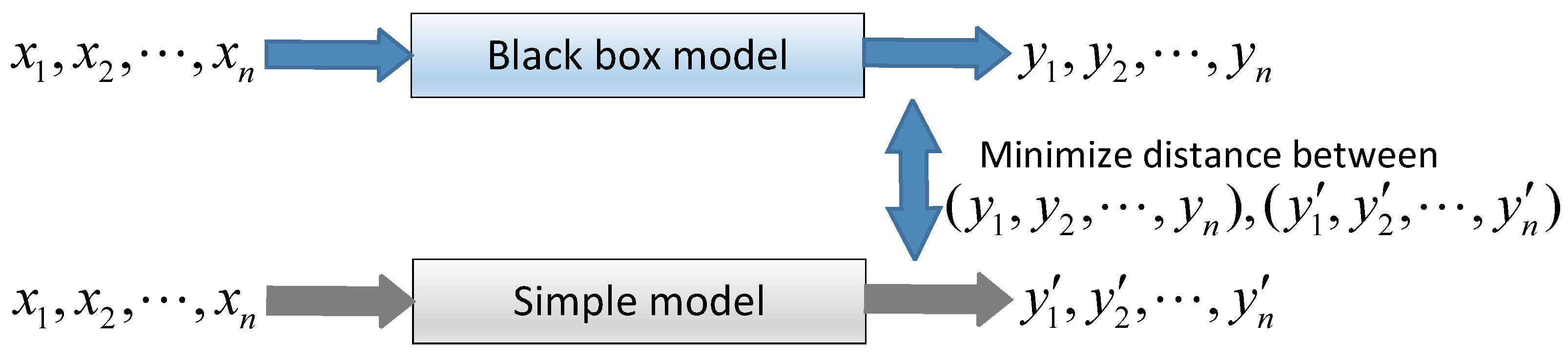
3.3.3. Mimic Model
4. Interpretable Machine Learning in Smart Grid
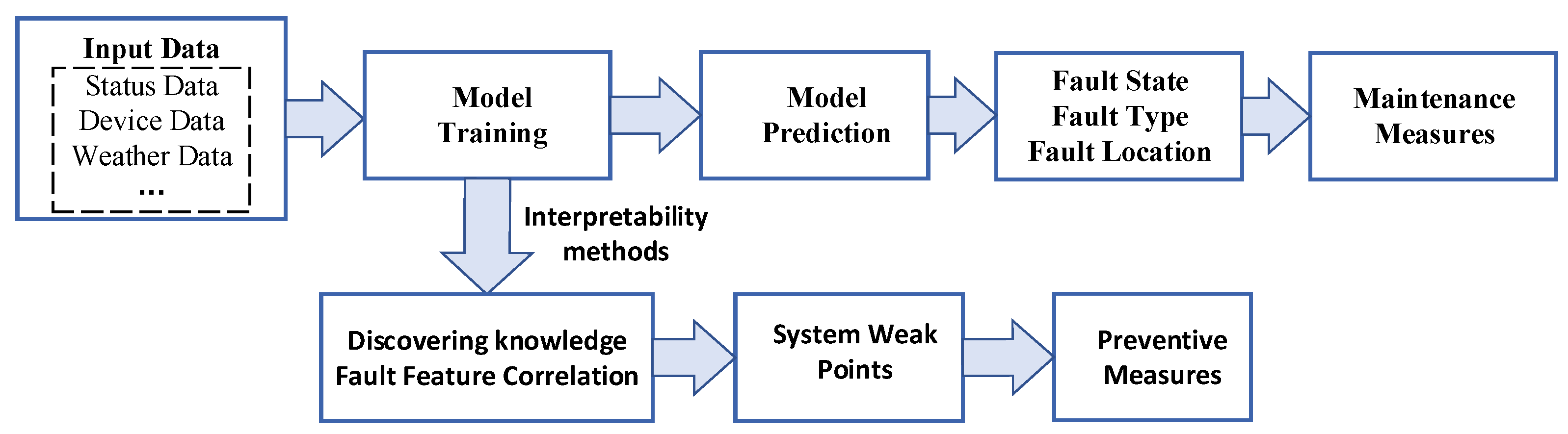
4.1. Fault Diagnosis
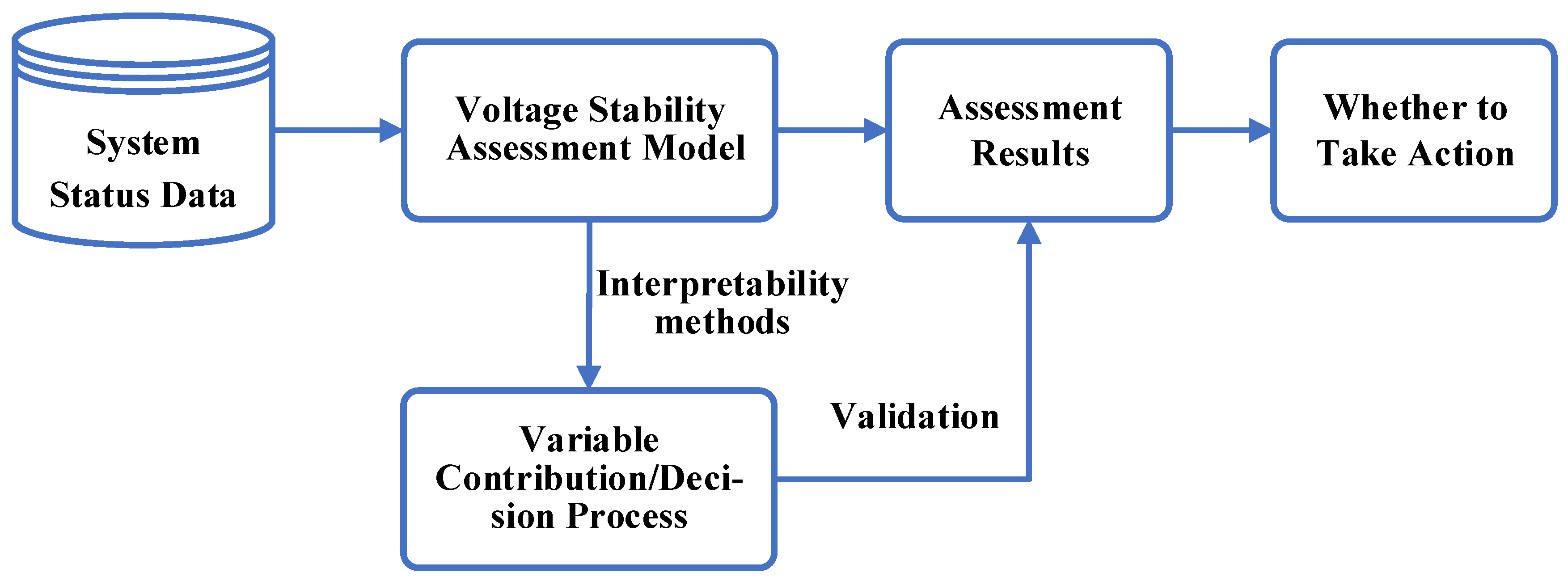
4.2. Security and Stability Analysis
4.3. Energy Forecasting
4.4. Power System Flexibility
4.5. Others
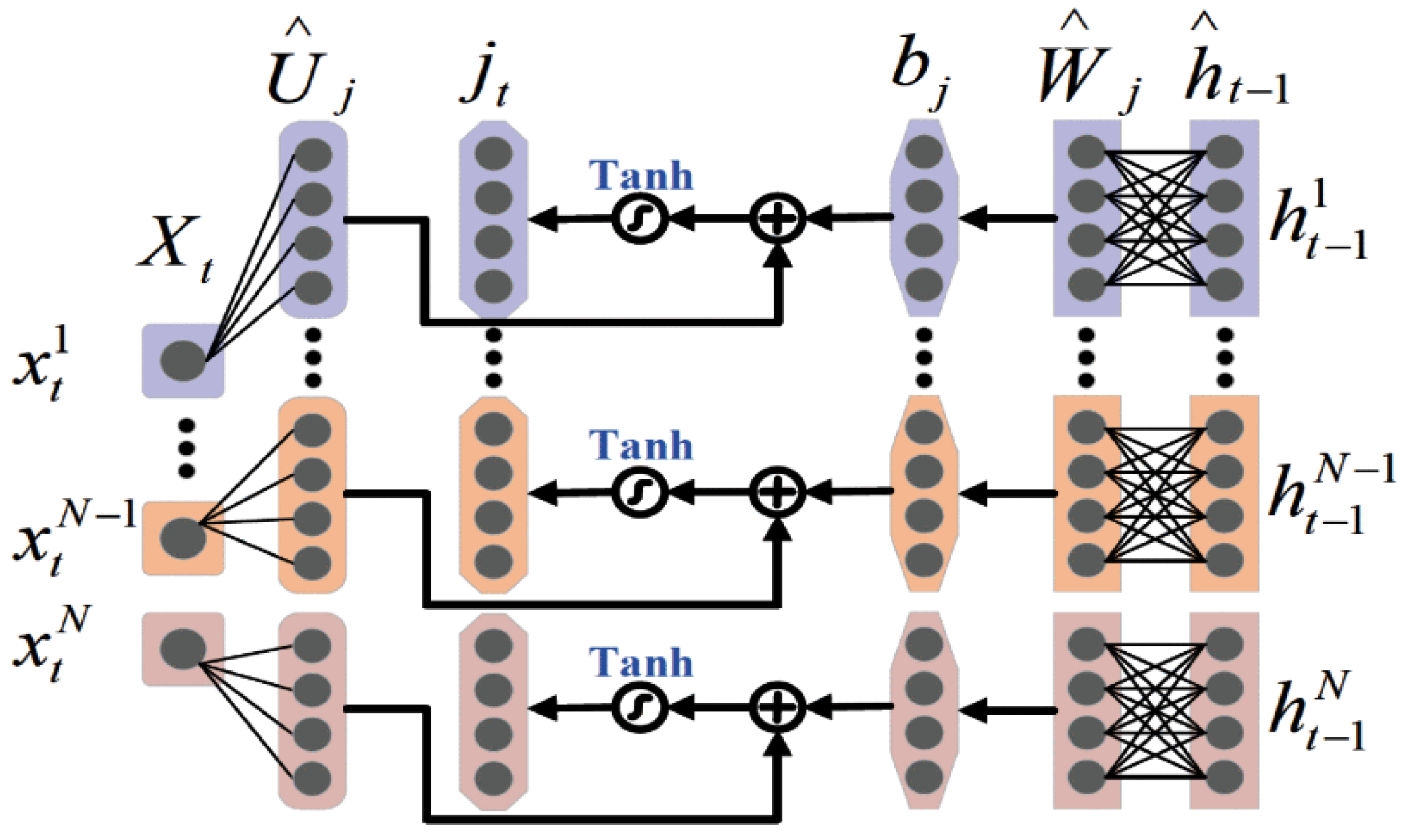
4.6. Case: Interpretable LSTM Model for Residential Load Forecasting
5. Future Research Directions
- Interpreting data: The smart grid field uses data from a variety of different sources, including various signals collected in real time from the power system, user information, device data, weather data, and more. Most of the published research focuses on the performance and interpretation of prediction models, ignoring the exploration and understanding of the data. Knowing what is behind the data can help you choose and explore a more suitable model later.
- Embedding domain knowledge: Most ML models in the smart grid provide prediction results using a data-driven approach. Domain knowledge may only be used to validate model decisions rather than being incorporated into models to participate in decision inference. If we embed domain knowledge into model inference, we can obtain more informative explanations. Therefore, it is a promising research direction to combine human knowledge, such as in the form of a knowledge graph, with ML technology to build interpretable ML models.
- Developing more in-model interpretability methods: Benefiting from the excellent characterization performance, complex DL models have been applied to different areas of the smart grid. It is advisable to verify the reliability of the model through post-hoc analysis of feature contributions. However, there is still an open question on how to build intrinsically interpretable deep neural networks without degrading model performance. In fact, post-model interpretability methods are always difficult to explain the model directly from the internal logic. They are only approximate interpretations of the model and may not be consistent with how the model actually predicted. Therefore, the use of these models in key decision-making areas requires careful consideration. Future work should develop more complex DL models with in-model interpretability.
- Generating human-centered interpretation: An ideal interpretability method should be able to make different interpretations according to the audience’s background knowledge and interpretation needs. At the same time, this interpretation should be the logical reasoning process behind the model while giving the decisions. Therefore, extensive research is required to establish appropriate methods to provide personalized interpretations based on the expected user’s expertise and abilities.
- Develop interpretable time series models: Most studies of interpretability methods are on images. However, in smart grid applications, much information such as current, load, etc., exists in the form of time series. Therefore, we urgently need to study interpretable ML applied to time series models.
- Applying interpretable ML to more critical areas: In addition to the applications mentioned in the paper, we believe that power dispatch and control, power safety operations, and other user-oriented fields require more support for interpretability.
6. Conclusions
Author Contributions
Funding
Conflicts of Interest
Abbreviations
| AC | Air conditioning |
| ACE | Automatic concept interpretation |
| AI | Artificial intelligence |
| CAM | Class activation map |
| CNN | Convolution neural network |
| CPES | Cyber-physical energy system |
| DBN | Deep belief network |
| DeConvNet | Deconvolution network |
| DL | Deep learning |
| DNN | Deep neural network |
| DSGC | Decentral smart grid control |
| DT | Decision tree |
| EDA | Exploratory data analysis |
| GAM | Generalized additive model |
| GCN | Graph convolutional network |
| GDPR | General Data Protection Regulation |
| GLM | Generalized linear model |
| GRU | Gated recurrent unit |
| HEMS | Home energy management system |
| HGAT | Heterogeneous graph attention network |
| ICE | Individual conditional expectation |
| IM-LSTM | Interpretable memristive LSTM |
| KNN | K-nearest neighbors |
| KPRN | Konwledge path recurrent network |
| LIME | Local interpretable model-agnostic explanation |
| LLI | Local mimic model-local linear interpretation |
| LR | Linear regression |
| LRP | Layer-wise relevance propagation |
| LSTM | Long short-term memory |
| ML | Machine learning |
| MLP | Multi-layer perceptron |
| NARX | Nonlinear autoregressive exogenous |
| NILM | Non-intrusive load monitoring |
| PCA | Principal component analysis |
| PDP | partial dependence plot |
| PINN | Physical information neural network |
| ReLU | Rectified linear unit |
| RF | Random forest |
| RL | Reinforcement learning |
| SAE | Stacked autoencoder |
| SHAP | Shapley additive explanations |
| SVM | Support vector machine |
| TCAV | Quantitative testing with concept activation vectors |
| TED | Teaching explanation for decisions |
| t-SNE | t-distributed stochastic neighbor embedding |
| XAI | Explainable artificial intelligence |
References
- Dileep, G. A survey on smart grid technologies and applications. Renew. Energy 2020, 146, 2589–2625. [Google Scholar] [CrossRef]
- Paul, S.; Rabbani, M.S.; Kundu, R.K.; Zaman, S.M.R. A review of smart technology (Smart Grid) and its features. In Proceedings of the 2014 1st International Conference on Non Conventional Energy (ICONCE 2014), Kalyani, India, 16–17 January 2014; IEEE: Piscataway, NJ, USA, 2014; pp. 200–203. [Google Scholar]
- Mollah, M.B.; Zhao, J.; Niyato, D.; Lam, K.Y.; Zhang, X.; Ghias, A.M.; Koh, L.H.; Yang, L. Blockchain for future smart grid: A comprehensive survey. IEEE Internet Things J. 2020, 8, 18–43. [Google Scholar] [CrossRef]
- Syed, D.; Zainab, A.; Ghrayeb, A.; Refaat, S.S.; Abu-Rub, H.; Bouhali, O. Smart grid big data analytics: Survey of technologies, techniques, and applications. IEEE Access 2020, 9, 59564–59585. [Google Scholar] [CrossRef]
- Hossain, E.; Khan, I.; Un-Noor, F.; Sikander, S.S.; Sunny, M.S.H. Application of big data and machine learning in smart grid, and associated security concerns: A review. IEEE Access 2019, 7, 13960–13988. [Google Scholar] [CrossRef]
- Azad, S.; Sabrina, F.; Wasimi, S. Transformation of smart grid using machine learning. In Proceedings of the 2019 29th Australasian Universities Power Engineering Conference (AUPEC), Nadi, Fiji, 26–29 November 2019; IEEE: Piscataway, NJ, USA, 2019; pp. 1–6. [Google Scholar]
- Sun, C.C.; Liu, C.C.; Xie, J. Cyber-physical system security of a power grid: State-of-the-art. Electronics 2016, 5, 40. [Google Scholar] [CrossRef] [Green Version]
- Yohanandhan, R.V.; Elavarasan, R.M.; Manoharan, P.; Mihet-Popa, L. Cyber-physical power system (CPPS): A review on modeling, simulation, and analysis with cyber security applications. IEEE Access 2020, 8, 151019–151064. [Google Scholar] [CrossRef]
- Ibrahim, M.S.; Dong, W.; Yang, Q. Machine learning driven smart electric power systems: Current trends and new perspectives. Appl. Energy 2020, 272, 115237. [Google Scholar] [CrossRef]
- Omitaomu, O.A.; Niu, H. Artificial intelligence techniques in smart grid: A survey. Smart Cities 2021, 4, 548–568. [Google Scholar] [CrossRef]
- Jordan, M.I.; Mitchell, T.M. Machine learning: Trends, perspectives, and prospects. Science 2015, 349, 255–260. [Google Scholar] [CrossRef]
- Dobson, A.J.; Barnett, A.G. An Introduction to Generalized Linear Models; Chapman and Hall/CRC: Boca Raton, FL, USA, 2018. [Google Scholar]
- Pisner, D.A.; Schnyer, D.M. Support vector machine. In Machine Learning; Elsevier: Amsterdam, The Netherlands, 2020; pp. 101–121. [Google Scholar]
- Deng, Z.; Zhu, X.; Cheng, D.; Zong, M.; Zhang, S. Efficient kNN classification algorithm for big data. Neurocomputing 2016, 195, 143–148. [Google Scholar] [CrossRef]
- Xu, R.; Wunsch, D. Survey of clustering algorithms. IEEE Trans. Neural Netw. 2005, 16, 645–678. [Google Scholar] [CrossRef] [Green Version]
- Myles, A.J.; Feudale, R.N.; Liu, Y.; Woody, N.A.; Brown, S.D. An introduction to decision tree modeling. J. Chemom. A J. Chemom. Soc. 2004, 18, 275–285. [Google Scholar] [CrossRef]
- Sagi, O.; Rokach, L. Ensemble learning: A survey. Wiley Interdiscip. Rev. Data Min. Knowl. Discov. 2018, 8, 1249. [Google Scholar] [CrossRef]
- Gurney, K. An Introduction to Neural Networks; CRC Press: Boca Raton, FL, USA, 2018. [Google Scholar]
- Doshi, D.; Khedkar, K.; Raut, N.; Kharde, S. Real Time Fault Failure Detection in Power Distribution Line using Power Line Communication. Int. J. Eng. Sci. 2016, 4834. [Google Scholar]
- Gu, C.; Li, H. Review on Deep Learning Research and Applications in Wind and Wave Energy. Energies 2022, 15, 1510. [Google Scholar] [CrossRef]
- You, S.; Zhao, Y.; Mandich, M.; Cui, Y.; Li, H.; Xiao, H.; Fabus, S.; Su, Y.; Liu, Y.; Yuan, H.; et al. A review on artificial intelligence for grid stability assessment. In Proceedings of the 2020 IEEE International Conference on Communications, Control, and Computing Technologies for Smart Grids (SmartGridComm), Tempe, AZ, USA, 11–13 November 2020; IEEE: Piscataway, NJ, USA, 2020; pp. 1–6. [Google Scholar]
- LeCun, Y.; Bengio, Y.; Hinton, G. Deep learning. Nature 2015, 521, 436–444. [Google Scholar] [CrossRef]
- Baldi, P. Autoencoders, unsupervised learning, and deep architectures. In Proceedings of the ICML Workshop on Unsupervised and Transfer Learning, JMLR Workshop and Conference Proceedings, Bellevue, WA, USA, 27 June 2012; pp. 37–49. [Google Scholar]
- Aloysius, N.; Geetha, M. A review on deep convolutional neural networks. In Proceedings of the 2017 International Conference on Communication and Signal Processing (ICCSP), Chennai, India, 6–8 April 2017; IEEE: Piscataway, NJ, USA, 2017; pp. 588–592. [Google Scholar]
- Yu, Y.; Si, X.; Hu, C.; Zhang, J. A review of recurrent neural networks: LSTM cells and network architectures. Neural Comput. 2019, 31, 1235–1270. [Google Scholar] [CrossRef]
- Cremer, J.L.; Konstantelos, I.; Strbac, G. From optimization-based machine learning to interpretable security rules for operation. IEEE Trans. Power Syst. 2019, 34, 3826–3836. [Google Scholar] [CrossRef]
- IqtiyaniIlham, N.; Hasanuzzaman, M.; Hosenuzzaman, M. European smart grid prospects, policies, and challenges. Renew. Sustain. Energy Rev. 2017, 67, 776–790. [Google Scholar] [CrossRef]
- Eskandarpour, R.; Khodaei, A. Machine learning based power grid outage prediction in response to extreme events. IEEE Trans. Power Syst. 2016, 32, 3315–3316. [Google Scholar] [CrossRef]
- Lundberg, J.; Lundborg, A. Using Opaque AI for Smart Grids. Bachelor’s Thesis, Department of Informatics, Lund University, Lund, Sweden, 2020. [Google Scholar]
- Ren, C.; Xu, Y.; Zhang, R. An Interpretable Deep Learning Method for Power System Dynamic Security Assessment via Tree Regularization. IEEE Trans. Power Syst. 2021. [Google Scholar] [CrossRef]
- Ahmad, M.A.; Eckert, C.; Teredesai, A. Interpretable machine learning in healthcare. In Proceedings of the 2018 ACM International Conference on Bioinformatics, Computational Biology, and Health Informatics, Washington, DC, USA, 29 August–1 September 2018; pp. 559–560. [Google Scholar]
- Garreau, D.; Luxburg, U. Explaining the explainer: A first theoretical analysis of LIME. In Proceedings of the International Conference on Artificial Intelligence and Statistics, PMLR, Online, 26–28 August 2020; pp. 1287–1296. [Google Scholar]
- Mokhtari, K.E.; Higdon, B.P.; Başar, A. Interpreting financial time series with SHAP values. In Proceedings of the 29th Annual International Conference on Computer Science and Software Engineering, Markham, ON, Canada, 4–6 November 2019; pp. 166–172. [Google Scholar]
- Tjoa, E.; Guan, C. A survey on explainable artificial intelligence (xai): Toward medical xai. IEEE Trans. Neural Netw. Learn. Syst. 2020, 32, 4793–4813. [Google Scholar] [CrossRef]
- Watson, D.S. Interpretable machine learning for genomics. Hum. Genet. 2021. [Google Scholar] [CrossRef]
- Rutkowski, T. Explainable Artificial Intelligence Based on Neuro-Fuzzy Modeling with Applications in Finance; Springer Nature: Berlin, Germany, 2021; Volume 964. [Google Scholar]
- Omeiza, D.; Webb, H.; Jirotka, M.; Kunze, L. Explanations in autonomous driving: A survey. IEEE Trans. Intell. Transp. Syst. 2021. [Google Scholar] [CrossRef]
- Doshi-Velez, F.; Kim, B. Towards a rigorous science of interpretable machine learning. arXiv 2017, arXiv:1702.08608. [Google Scholar]
- Gilpin, L.H.; Bau, D.; Yuan, B.Z.; Bajwa, A.; Specter, M.; Kagal, L. Explaining explanations: An overview of interpretability of machine learning. In Proceedings of the 2018 IEEE 5th International Conference on Data Science and Advanced Analytics (DSAA), Turin, Italy, 1–3 October 2018; IEEE: Piscataway, NJ, USA, 2018; pp. 80–89. [Google Scholar]
- Arrieta, A.B.; Díaz-Rodríguez, N.; Del Ser, J.; Bennetot, A.; Tabik, S.; Barbado, A.; García, S.; Gil-López, S.; Molina, D.; Benjamins, R.; et al. Explainable Artificial Intelligence (XAI): Concepts, taxonomies, opportunities and challenges toward responsible AI. Inf. Fusion 2020, 58, 82–115. [Google Scholar] [CrossRef] [Green Version]
- Rudin, C.; Chen, C.; Chen, Z.; Huang, H.; Semenova, L.; Zhong, C. Interpretable machine learning: Fundamental principles and 10 grand challenges. Stat. Surv. 2022, 16, 1–85. [Google Scholar] [CrossRef]
- Guidotti, R.; Monreale, A.; Ruggieri, S.; Turini, F.; Giannotti, F.; Pedreschi, D. A survey of methods for explaining black box models. ACM Comput. Surv. (CSUR) 2018, 51, 1–42. [Google Scholar] [CrossRef] [Green Version]
- Shortliffe, E.H.; Buchanan, B.G. A model of inexact reasoning in medicine. Math. Biosci. 1975, 23, 351–379. [Google Scholar] [CrossRef]
- Laurent, H.; Rivest, R.L. Constructing optimal binary decision trees is NP-complete. Inf. Process. Lett. 1976, 5, 15–17. [Google Scholar]
- Rivest, R.L. Learning decision lists. Mach. Learn. 1987, 2, 229–246. [Google Scholar] [CrossRef] [Green Version]
- Petch, J.; Di, S.; Nelson, W. Opening the black box: The promise and limitations of explainable machine learning in cardiology. Can. J. Cardiol. 2021, 38, 204–213. [Google Scholar] [CrossRef]
- Goldstein, A.; Kapelner, A.; Bleich, J.; Pitkin, E. Peeking inside the black box: Visualizing statistical learning with plots of individual conditional expectation. J. Comput. Graph. Stat. 2015, 24, 44–65. [Google Scholar] [CrossRef]
- Craven, M.; Shavlik, J. Extracting tree-structured representations of trained networks. Adv. Neural Inf. Process. Syst. 1995, 8, 24–30. [Google Scholar]
- Watson, D.S.; Floridi, L. The explanation game: A formal framework for interpretable machine learning. In Ethics, Governance, and Policies in Artificial Intelligence; Springer: Berlin/Heidelberg, Germany, 2021; pp. 185–219. [Google Scholar]
- Zhang, Y.; Tiňo, P.; Leonardis, A.; Tang, K. A survey on neural network interpretability. IEEE Trans. Emerg. Top. Comput. Intell. 2021. [Google Scholar] [CrossRef]
- Chen, N.; Ribeiro, B.; Chen, A. Financial credit risk assessment: A recent review. Artif. Intell. Rev. 2016, 45, 1–23. [Google Scholar] [CrossRef]
- Obermeyer, Z.; Powers, B.; Vogeli, C.; Mullainathan, S. Dissecting racial bias in an algorithm used to manage the health of populations. Science 2019, 366, 447–453. [Google Scholar] [CrossRef] [Green Version]
- Tsamados, A.; Aggarwal, N.; Cowls, J.; Morley, J.; Roberts, H.; Taddeo, M.; Floridi, L. The ethics of algorithms: Key problems and solutions. AI Soc. 2022, 37, 215–230. [Google Scholar] [CrossRef]
- Zhao, X.; Banks, A.; Sharp, J.; Robu, V.; Flynn, D.; Fisher, M.; Huang, X. A safety framework for critical systems utilising deep neural networks. In International Conference on Computer Safety, Reliability, and Security; Springer: Berlin/Heidelberg, Germany, 2020; pp. 244–259. [Google Scholar]
- Li, L.; Ota, K.; Dong, M. When Weather Matters: IoT-Based Electrical Load Forecasting for Smart Grid. IEEE Commun. Mag. 2017, 55, 46–51. [Google Scholar] [CrossRef] [Green Version]
- Van Cutsem, T.; Vournas, C. Voltage Stability of Electric Power Systems; Springer Science & Business Media: New York, NY, USA, 2007. [Google Scholar]
- Furse, C.M.; Kafal, M.; Razzaghi, R.; Shin, Y.J. Fault diagnosis for electrical systems and power networks: A review. IEEE Sens. J. 2020, 21, 888–906. [Google Scholar] [CrossRef]
- Robnik-Šikonja, M.; Bohanec, M. Perturbation-based explanations of prediction models. In Human and Machine Learning; Springer: Berlin/Heidelberg, Germany, 2018; pp. 159–175. [Google Scholar]
- Carvalho, D.V.; Pereira, E.M.; Cardoso, J.S. Machine learning interpretability: A survey on methods and metrics. Electronics 2019, 8, 832. [Google Scholar] [CrossRef] [Green Version]
- Tukey, J.W. Exploratory Data Analysis; Pearson: Reading, MA, USA, 1977; Volume 2. [Google Scholar]
- Liu, H.; Zhong, C.; Alnusair, A.; Islam, S.R. FAIXID: A framework for enhancing ai explainability of intrusion detection results using data cleaning techniques. J. Netw. Syst. Manag. 2021, 29, 1–30. [Google Scholar] [CrossRef]
- Kandel, S.; Paepcke, A.; Hellerstein, J.M.; Heer, J. Enterprise data analysis and visualization: An interview study. IEEE Trans. Vis. Comput. Graph. 2012, 18, 2917–2926. [Google Scholar] [CrossRef] [PubMed] [Green Version]
- Artac, M.; Jogan, M.; Leonardis, A. Incremental PCA for on-line visual learning and recognition. In Proceedings of the 2002 International Conference on Pattern Recognition, Quebec City, QC, Canada, 11–15 August 2002; IEEE: Piscataway, NJ, USA, 2002; Volume 3, pp. 781–784. [Google Scholar]
- Wattenberg, M.; Viégas, F.; Johnson, I. How to use t-SNE effectively. Distill 2016, 1, e2. [Google Scholar] [CrossRef]
- Benesty, J.; Chen, J.; Huang, Y.; Cohen, I. Pearson correlation coefficient. In Noise Reduction in Speech Processing; Springer: Berlin/Heidelberg, Germany, 2009; pp. 1–4. [Google Scholar]
- Ramsey, P.H. Critical values for Spearman’s rank order correlation. J. Educ. Stat. 1989, 14, 245–253. [Google Scholar]
- Ahmed, M. Data summarization: A survey. Knowl. Inf. Syst. 2019, 58, 249–273. [Google Scholar] [CrossRef]
- Kleindessner, M.; Awasthi, P.; Morgenstern, J. Fair k-center clustering for data summarization. In Proceedings of the International Conference on Machine Learning, PMLR, Long Beach, CA, USA, 10–15 June 2019; pp. 3448–3457. [Google Scholar]
- Hadi, Y.; Essannouni, F.; Thami, R.O.H. Video summarization by k-medoid clustering. In Proceedings of the 2006 ACM Symposium on Applied Computing, Dijon, France, 23–27 April 2006; pp. 1400–1401. [Google Scholar]
- Wang, K.; Zhang, J.; Li, D.; Zhang, X.; Guo, T. Adaptive affinity propagation clustering. arXiv 2008, arXiv:0805.1096. [Google Scholar]
- Kim, B.; Khanna, R.; Koyejo, O.O. Examples are not enough, learn to criticize! criticism for interpretability. Adv. Neural Inf. Process. Syst. 2016, 29, 2288–2296. [Google Scholar]
- Nelder, J.A.; Wedderburn, R.W. Generalized linear models. J. R. Stat. Soc. Ser. A 1972, 135, 370–384. [Google Scholar] [CrossRef]
- Hastie, T.J.; Tibshirani, R.J. Generalized Additive Models; Routledge: London, UK, 2017. [Google Scholar]
- Lou, Y.; Caruana, R.; Gehrke, J.; Hooker, G. Accurate intelligible models with pairwise interactions. In Proceedings of the 19th ACM SIGKDD International Conference on Knowledge Discovery and Data Mining, Chicago, IL, USA, 11–14 August 2013; pp. 623–631. [Google Scholar]
- Sun, R. Robust reasoning: Integrating rule-based and similarity-based reasoning. Artif. Intell. 1995, 75, 241–295. [Google Scholar] [CrossRef]
- Liu, B.; Hsu, W.; Ma, Y. Integrating Classification and Association Rule Mining. In Proceedings of the KDD’98: Proceedings of the Fourth International Conference on Knowledge Discovery and Data Mining, New York, NY, USA, 27–31 August 1998; Volume 98, pp. 80–86. [Google Scholar]
- Gacto, M.J.; Alcalá, R.; Herrera, F. Interpretability of linguistic fuzzy rule-based systems: An overview of interpretability measures. Inf. Sci. 2011, 181, 4340–4360. [Google Scholar] [CrossRef]
- Weinberger, K.Q.; Blitzer, J.; Saul, L. Distance metric learning for large margin nearest neighbor classification. Adv. Neural Inf. Process. Syst. 2005, 18. [Google Scholar]
- Sabour, S.; Frosst, N.; Hinton, G.E. Dynamic routing between capsules. Adv. Neural Inf. Process. Syst. 2017, 30. [Google Scholar]
- Raissi, M.; Perdikaris, P.; Karniadakis, G.E. Physics-informed neural networks: A deep learning framework for solving forward and inverse problems involving nonlinear partial differential equations. J. Comput. Phys. 2019, 378, 686–707. [Google Scholar] [CrossRef]
- Wang, X.; Wang, D.; Xu, C.; He, X.; Cao, Y.; Chua, T.S. Explainable reasoning over knowledge graphs for recommendation. In Proceedings of the AAAI conference on Artificial Intelligence, Honolulu, HI, USA, 27 January–1 February 2019; Volume 33, pp. 5329–5336. [Google Scholar]
- Cho, K.; van Merrienboer, B.; Gulcehre, C.; Bougares, F.; Schwenk, H.; Bengio, Y. Learning phrase representations using RNN encoder-decoder for statistical machine translation. In Proceedings of the Conference on Empirical Methods in Natural Language Processing (EMNLP 2014), Doha, Qatar, 25–29 October 2014. [Google Scholar]
- Lei, T.; Barzilay, R.; Jaakkola, T. Rationalizing neural predictions. arXiv 2016, arXiv:1606.04155. [Google Scholar]
- Hendricks, L.A.; Akata, Z.; Rohrbach, M.; Donahue, J.; Schiele, B.; Darrell, T. Generating visual explanations. In European Conference on Computer Vision; Springer: Berlin/Heidelberg, Germany, 2016; pp. 3–19. [Google Scholar]
- Park, D.H.; Hendricks, L.A.; Akata, Z.; Rohrbach, A.; Schiele, B.; Darrell, T.; Rohrbach, M. Multimodal explanations: Justifying decisions and pointing to the evidence. In Proceedings of the IEEE Conference on Computer Vision and Pattern Recognition, Salt Lake City, UT, USA, 18–23 June 2018; IEEE: Piscataway, NJ, USA, 2018; pp. 8779–8788. [Google Scholar]
- Hind, M.; Wei, D.; Campbell, M.; Codella, N.C.; Dhurandhar, A.; Mojsilović, A.; Natesan Ramamurthy, K.; Varshney, K.R. TED: Teaching AI to explain its decisions. In Proceedings of the 2019 AAAI/ACM Conference on AI, Ethics, and Society, Honolulu, HI, USA, 27–28 January 2019; pp. 123–129. [Google Scholar]
- Linardatos, P.; Papastefanopoulos, V.; Kotsiantis, S. Explainable ai: A review of machine learning interpretability methods. Entropy 2020, 23, 18. [Google Scholar] [CrossRef] [PubMed]
- Zeiler, M.D.; Fergus, R. Visualizing and understanding convolutional networks. In European Conference on Computer Vision; Springer: Berlin/Heidelberg, Germany, 2014; pp. 818–833. [Google Scholar]
- Bau, D.; Zhu, J.Y.; Strobelt, H.; Lapedriza, A.; Zhou, B.; Torralba, A. Understanding the Role of Individual Units in a Deep Neural Network. Proc. Natl. Acad. Sci. USA 2020, 117, 30071–30078. [Google Scholar] [CrossRef]
- Dalvi, F.; Durrani, N.; Sajjad, H.; Belinkov, Y.; Bau, A.; Glass, J. What Is One Grain of Sand in the Desert? Analyzing Individual Neurons in Deep NLP Models. Proc. AAAI Conf. Artif. Intell. 2019, 33, 6309–6317. [Google Scholar] [CrossRef] [Green Version]
- Montavon, G.; Samek, W.; Müller, K.R. Methods for interpreting and understanding deep neural networks. Digit. Signal Process. 2018, 73, 1–15. [Google Scholar] [CrossRef]
- Cafri, G.; Bailey, B.A. Understanding variable effects from black box prediction: Quantifying effects in tree ensembles using partial dependence. J. Data Sci. 2016, 14, 67–95. [Google Scholar] [CrossRef]
- Molnar, C. Interpretable Machine Learning; Lulu: Morrisville, NC, USA, 2020. [Google Scholar]
- Koh, P.W.; Liang, P. Understanding black-box predictions via influence functions. In Proceedings of the International Conference on Machine Learning, PMLR, Sydney, NSW, Australia, 6–11 August 2017; pp. 1885–1894. [Google Scholar]
- Robnik-Šikonja, M.; Kononenko, I. Explaining classifications for individual instances. IEEE Trans. Knowl. Data Eng. 2008, 20, 589–600. [Google Scholar] [CrossRef] [Green Version]
- Fong, R.C.; Vedaldi, A. Interpretable explanations of black boxes by meaningful perturbation. In Proceedings of the IEEE International Conference on Computer Vision, Venice, Italy, 22–29 October 2017; IEEE: Piscataway, NJ, USA, 2017; pp. 3429–3437. [Google Scholar]
- Simonyan, K.; Vedaldi, A.; Zisserman, A. Deep inside convolutional networks: Visualising image classification models and saliency maps. arXiv 2013, arXiv:1312.6034. [Google Scholar]
- Springenberg, J.T.; Dosovitskiy, A.; Brox, T.; Riedmiller, M. Striving for simplicity: The all convolutional net. arXiv 2014, arXiv:1412.6806. [Google Scholar]
- Sundararajan, M.; Taly, A.; Yan, Q. Axiomatic attribution for deep networks. In Proceedings of the International Conference on Machine Learning, PMLR, Sydney, NSW, Australia, 6–11 August 2017; pp. 3319–3328. [Google Scholar]
- Adebayo, J.; Gilmer, J.; Goodfellow, I.; Kim, B. Local explanation methods for deep neural networks lack sensitivity to parameter values. arXiv 2018, arXiv:1810.03307. [Google Scholar]
- Bach, S.; Binder, A.; Montavon, G.; Klauschen, F.; Müller, K.R.; Samek, W. On pixel-wise explanations for non-linear classifier decisions by layer-wise relevance propagation. PLoS ONE 2015, 10, e0130140. [Google Scholar] [CrossRef] [Green Version]
- Shrikumar, A.; Greenside, P.; Kundaje, A. Learning important features through propagating activation differences. In Proceedings of the International Conference on Machine Learning, PMLR, Sydney, NSW, Australia, 6–11 August 2017 2017; pp. 3145–3153. [Google Scholar]
- Lundberg, S.M.; Lee, S.I. A unified approach to interpreting model predictions. Adv. Neural Inf. Process. Syst. 2017, 30. [Google Scholar]
- Lundberg, S.M.; Erion, G.G.; Lee, S.I. Consistent individualized feature attribution for tree ensembles. arXiv 2018, arXiv:1802.03888. [Google Scholar]
- Zhou, B.; Khosla, A.; Lapedriza, A.; Oliva, A.; Torralba, A. Learning deep features for discriminative localization. In Proceedings of the IEEE Conference on Computer Vision and Pattern Recognition, Las Vegas, NV, USA, 27–30 June 2016; IEEE: Piscataway, NJ, USA, 2016; pp. 2921–2929. [Google Scholar]
- Selvaraju, R.R.; Cogswell, M.; Das, A.; Vedantam, R.; Parikh, D.; Batra, D. Grad-cam: Visual explanations from deep networks via gradient-based localization. In Proceedings of the IEEE International Conference on Computer Vision, Venice, Italy, 22–29 October 2017; IEEE: Piscataway, NJ, USA, 2017; pp. 618–626. [Google Scholar]
- Chattopadhay, A.; Sarkar, A.; Howlader, P.; Balasubramanian, V.N. Grad-cam++: Generalized gradient-based visual explanations for deep convolutional networks. In Proceedings of the 2018 IEEE Winter Conference on Applications of Computer Vision (WACV), Lake Tahoe, NV, USA, 12–15 March 2018; IEEE: Piscataway, NJ, USA, 2018; pp. 839–847. [Google Scholar]
- Kim, B.; Wattenberg, M.; Gilmer, J.; Cai, C.; Wexler, J.; Viegas, F. Interpretability beyond feature attribution: Quantitative testing with concept activation vectors (tcav). In Proceedings of the International Conference on Machine Learning, PMLR, Stockholm, Sweden, 10–15 July 2018; pp. 2668–2677. [Google Scholar]
- Ghorbani, A.; Wexler, J.; Zou, J.Y.; Kim, B. Towards automatic concept-based explanations. Adv. Neural Inf. Process. Syst. 2019, 32. [Google Scholar]
- Verma, S.; Dickerson, J.; Hines, K. Counterfactual explanations for machine learning: A review. arXiv 2020, arXiv:2010.10596. [Google Scholar]
- Tan, S.; Caruana, R.; Hooker, G.; Lou, Y. Distill-and-compare: Auditing black-box models using transparent model distillation. In Proceedings of the 2018 AAAI/ACM Conference on AI, Ethics, and Society, New Orleans, LA, USA, 1–3 August 2018; pp. 303–310. [Google Scholar]
- Wu, M.; Hughes, M.; Parbhoo, S.; Zazzi, M.; Roth, V.; Doshi-Velez, F. Beyond sparsity: Tree regularization of deep models for interpretability. In Proceedings of the AAAI Conference on Artificial Intelligence, New Orleans, LA, USA, 1–3 August 2018; Volume 32. [Google Scholar]
- Ribeiro, M.T.; Singh, S.; Guestrin, C. “Why should I trust you?” Explaining the predictions of any classifier. In Proceedings of the 22nd ACM SIGKDD International Conference on Knowledge Discovery and Data Mining, San Francisco, CA, USA, 13–17 August 2016; pp. 1135–1144. [Google Scholar]
- Zafar, M.R.; Khan, N.M. DLIME: A deterministic local interpretable model-agnostic explanations approach for computer-aided diagnosis systems. arXiv 2019, arXiv:1906.10263. [Google Scholar]
- Ribeiro, M.T.; Singh, S.; Guestrin, C. Anchors: High-precision model-agnostic explanations. In Proceedings of the AAAI Conference on Artificial Intelligence, New Orleans, LA, USA, 1–3 August 2018; Volume 32. [Google Scholar]
- Gevrey, M.; Dimopoulos, I.; Lek, S. Review and comparison of methods to study the contribution of variables in artificial neural network models. Ecol. Model. 2003, 160, 249–264. [Google Scholar] [CrossRef]
- Montavon, G.; Binder, A.; Lapuschkin, S.; Samek, W.; Müller, K.R. Layer-wise relevance propagation: An overview. In Explainable AI: Interpreting, Explaining and Visualizing Deep Learning; Springer: Berlin/Heidelberg, Germany, 2019; pp. 193–209. [Google Scholar]
- Wachter, S.; Mittelstadt, B.; Russell, C. Counterfactual explanations without opening the black box: Automated decisions and the GDPR. Harv. JL Tech. 2017, 31, 841. [Google Scholar] [CrossRef] [Green Version]
- Bastani, O.; Kim, C.; Bastani, H. Interpretability via model extraction. arXiv 2017, arXiv:1706.09773. [Google Scholar]
- Che, Z.; Purushotham, S.; Khemani, R.; Liu, Y. Distilling knowledge from deep networks with applications to healthcare domain. arXiv 2015, arXiv:1512.03542. [Google Scholar]
- Tan, S.; Caruana, R.; Hooker, G.; Koch, P.; Gordo, A. Learning global additive explanations for neural nets using model distillation. In Proceedings of the CLR 2019 Conference, Minneapolis, MN, USA, 3–5 June 2019. [Google Scholar]
- Jiang, H.; Zhang, J.J.; Gao, W.; Wu, Z. Fault detection, identification, and location in smart grid based on data-driven computational methods. IEEE Trans. Smart Grid 2014, 5, 2947–2956. [Google Scholar] [CrossRef]
- Shi, Z.; Yao, W.; Li, Z.; Zeng, L.; Zhao, Y.; Zhang, R.; Tang, Y.; Wen, J. Artificial intelligence techniques for stability analysis and control in smart grids: Methodologies, applications, challenges and future directions. Appl. Energy 2020, 278, 115733. [Google Scholar] [CrossRef]
- Ardito, C.; Deldjoo, Y.; Sciascio, E.D.; Nazary, F.; Sapienza, G. ISCADA: Towards a Framework for Interpretable Fault Prediction in Smart Electrical Grids. In IFIP Conference on Human-Computer Interaction; Springer: Berlin/Heidelberg, Germany, 2021; pp. 270–274. [Google Scholar]
- Kim, S.G.; Ryu, S.; Kim, H.; Jin, K.; Cho, J. Enhancing the Explainability of AI Models in Nuclear Power Plants with Layer-wise Relevance Propagation. In Proceedings of the Transactions of the Korean Nuclear Society Virtual Autumn Meeting, Jeju, Korea, 21–22 October 2021. [Google Scholar]
- Zhang, K.; Xu, P.; Gao, T.; ZHANG, J. A Trustworthy Framework of Artificial Intelligence for Power Grid Dispatching Systems. In Proceedings of the 2021 IEEE 1st International Conference on Digital Twins and Parallel Intelligence (DTPI), Beijing, China, 15 July–15 August 2021; IEEE: Piscataway, NJ, USA, 2021; pp. 418–421. [Google Scholar]
- Liu, Y.; Zhang, N.; Wu, D.; Botterud, A.; Yao, R.; Kang, C. Searching for critical power system cascading failures with graph convolutional network. IEEE Trans. Control Netw. Syst. 2021, 8, 1304–1313. [Google Scholar] [CrossRef]
- Wali, S.; Khan, I. Explainable Signature-based Machine Learning Approach for Identification of Faults in Grid-Connected Photovoltaic Systems. arXiv 2021, arXiv:2112.14842. [Google Scholar]
- Zhang, D.; Li, C.; Shahidehpour, M.; Wu, Q.; Zhou, B.; Zhang, C.; Huang, W. A bi-level machine learning method for fault diagnosis of oil-immersed transformers with feature explainability. Int. J. Electr. Power Energy Syst. 2022, 134, 107356. [Google Scholar] [CrossRef]
- Zhu, L.; Lu, C.; Kamwa, I.; Zeng, H. Spatial–temporal feature learning in smart grids: A case study on short-term voltage stability assessment. IEEE Trans. Ind. Informatics 2018, 16, 1470–1482. [Google Scholar] [CrossRef]
- Wu, S.; Zheng, L.; Hu, W.; Yu, R.; Liu, B. Improved deep belief network and model interpretation method for power system transient stability assessment. J. Mod. Power Syst. Clean Energy 2019, 8, 27–37. [Google Scholar] [CrossRef]
- Gorzałczany, M.B.; Piekoszewski, J.; Rudziński, F. A modern data-mining approach based on genetically optimized fuzzy systems for interpretable and accurate smart-grid stability prediction. Energies 2020, 13, 2559. [Google Scholar] [CrossRef]
- Kruse, J.; Schäfer, B.; Witthaut, D. Exploring deterministic frequency deviations with explainable AI. In Proceedings of the 2021 IEEE International Conference on Communications, Control, and Computing Technologies for Smart Grids (SmartGridComm), Aachen, Germany, 25–28 October 2021; IEEE: Piscataway, NJ, USA, 2021; pp. 133–139. [Google Scholar]
- Kruse, J.; Schäfer, B.; Witthaut, D. Revealing drivers and risks for power grid frequency stability with explainable AI. Patterns 2021, 2, 100365. [Google Scholar] [CrossRef]
- Wang, Z.; Zhou, Y.; Guo, Q.; Sun, H. Interpretable neighborhood deep models for online total transfer capability evaluation of power systems. IEEE Trans. Power Syst. 2021, 37, 260–271. [Google Scholar] [CrossRef]
- Kaur, D.; Islam, S.N.; Mahmud, M.; Dong, Z. Energy forecasting in smart grid systems: A review of the state-of-the-art techniques. arXiv 2020, arXiv:2011.12598. [Google Scholar]
- Fan, C.; Xiao, F.; Yan, C.; Liu, C.; Li, Z.; Wang, J. A novel methodology to explain and evaluate data-driven building energy performance models based on interpretable machine learning. Appl. Energy 2019, 235, 1551–1560. [Google Scholar] [CrossRef]
- Kim, T.Y.; Cho, S.B. Predicting residential energy consumption using CNN-LSTM neural networks. Energy 2019, 182, 72–81. [Google Scholar] [CrossRef]
- Kim, J.Y.; Cho, S.B. Electric energy consumption prediction by deep learning with state explainable autoencoder. Energies 2019, 12, 739. [Google Scholar] [CrossRef] [Green Version]
- Grimaldo, A.I.; Novak, J. Combining machine learning with visual analytics for explainable forecasting of energy demand in prosumer scenarios. Procedia Comput. Sci. 2020, 175, 525–532. [Google Scholar] [CrossRef]
- Kuzlu, M.; Cali, U.; Sharma, V.; Güler, Ö. Gaining insight into solar photovoltaic power generation forecasting utilizing explainable artificial intelligence tools. IEEE Access 2020, 8, 187814–187823. [Google Scholar] [CrossRef]
- Lu, Y.; Murzakhanov, I.; Chatzivasileiadis, S. Neural network interpretability for forecasting of aggregated renewable generation. In Proceedings of the 2021 IEEE International Conference on Communications, Control, and Computing Technologies for Smart Grids (SmartGridComm), Aachen, Germany, 25–28 October 2021; IEEE: Piscataway, NJ, USA, 2021; pp. 282–288. [Google Scholar]
- Wenninger, S.; Kaymakci, C.; Wiethe, C. Explainable long-term building energy consumption prediction using QLattice. Appl. Energy 2022, 308, 118300. [Google Scholar] [CrossRef]
- Li, C.; Dong, Z.; Ding, L.; Petersen, H.; Qiu, Z.; Chen, G.; Prasad, D. Interpretable Memristive LSTM Network Design for Probabilistic Residential Load Forecasting. IEEE Trans. Circuits Syst. I Regul. Pap. 2022, 69, 2297–2310. [Google Scholar] [CrossRef]
- Mohandes, B.; El Moursi, M.S.; Hatziargyriou, N.; El Khatib, S. A review of power system flexibility with high penetration of renewables. IEEE Trans. Power Syst. 2019, 34, 3140–3155. [Google Scholar] [CrossRef]
- Luo, X.; Dooner, M.; He, W.; Wang, J.; Li, Y.; Li, D.; Kiselychnyk, O. Feasibility study of a simulation software tool development for dynamic modelling and transient control of adiabatic compressed air energy storage with its electrical power system applications. Appl. Energy 2018, 228, 1198–1219. [Google Scholar] [CrossRef]
- Antonopoulos, I.; Robu, V.; Couraud, B.; Kirli, D.; Norbu, S.; Kiprakis, A.; Flynn, D.; Elizondo-Gonzalez, S.; Wattam, S. Artificial intelligence and machine learning approaches to energy demand-side response: A systematic review. Renew. Sustain. Energy Rev. 2020, 130, 109899. [Google Scholar] [CrossRef]
- Kouzelis, K.; Tan, Z.H.; Bak-Jensen, B.; Pillai, J.R.; Ritchie, E. Estimation of residential heat pump consumption for flexibility market applications. IEEE Trans. Smart Grid 2015, 6, 1852–1864. [Google Scholar] [CrossRef]
- Mathew, A.; Roy, A.; Mathew, J. Intelligent residential energy management system using deep reinforcement learning. IEEE Syst. J. 2020, 14, 5362–5372. [Google Scholar] [CrossRef]
- Kumar, H.; Mammen, P.M.; Ramamritham, K. Explainable ai: Deep reinforcement learning agents for residential demand side cost savings in smart grids. arXiv 2019, arXiv:1910.08719. [Google Scholar]
- Li, A.; Xiao, F.; Zhang, C.; Fan, C. Attention-based interpretable neural network for building cooling load prediction. Appl. Energy 2021, 299, 117238. [Google Scholar] [CrossRef]
- Kelly, J.; Knottenbelt, W. Neural nilm: Deep neural networks applied to energy disaggregation. In Proceedings of the 2nd ACM International Conference on Embedded Systems for Energy-Efficient Built Environments, Seoul, Korea, 4–5 November 2015; pp. 55–64. [Google Scholar]
- Houidi, S.; Fourer, D.; Auger, F. On the use of concentrated time–frequency representations as input to a deep convolutional neural network: Application to non intrusive load monitoring. Entropy 2020, 22, 911. [Google Scholar] [CrossRef]
- Murray, D.; Stankovic, L.; Stankovic, V. Explainable NILM networks. In Proceedings of the 5th International Workshop on Non-Intrusive Load Monitoring, Online, 18 November 2020; pp. 64–69. [Google Scholar]
- Wang, W.; Yu, N.; Shi, J.; Navarro, N. Diversity factor prediction for distribution feeders with interpretable machine learning algorithms. In Proceedings of the 2020 IEEE Power & Energy Society General Meeting (PESGM), Montreal, QC, Canada, 2–6 August 2020; IEEE: Piscataway, NJ, USA, 2020; pp. 1–5. [Google Scholar]
- Aryan, P.R.; Ekaputra, F.J.; Sabou, M.; Hauer, D.; Mosshammer, R.; Einfalt, A.; Miksa, T.; Rauber, A. Explainable cyber-physical energy systems based on knowledge graph. In Proceedings of the 9th Workshop on Modeling and Simulation of Cyber-Physical Energy Systems, Online, 18 May 2021; pp. 1–6. [Google Scholar]
- Toubeau, J.F.; Bottieau, J.; Wang, Y.; Vallee, F. Interpretable Probabilistic Forecasting of Imbalances in Renewable-Dominated Electricity Systems. IEEE Trans. Sustain. Energy 2021, 13, 1267–1277. [Google Scholar] [CrossRef]
- Zhang, K.; Zhang, J.; Xu, P.D.; Gao, T.; Gao, D.W. Explainable AI in Deep Reinforcement Learning Models for Power System Emergency Control. IEEE Trans. Comput. Soc. Syst. 2021, 9, 419–427. [Google Scholar] [CrossRef]
- Machlev, R.; Perl, M.; Belikov, J.; Levy, K.; Levron, Y. Measuring Explainability and Trustworthiness of Power Quality Disturbances Classifiers Using XAI-Explainable Artificial Intelligence. IEEE Trans. Ind. Informatics 2021, 18, 5127–5137. [Google Scholar] [CrossRef]
- Khan, A.A.; Beg, O.A.; Jin, Y.; Ahmed, S. An Explainable Intelligent Framework for Anomaly Mitigation in Cyber-Physical Inverter-based Systems. arXiv 2022, arXiv:17912006.v1. [Google Scholar]


| Type | Medium | Representative Method | Interpretation Form |
|---|---|---|---|
| Interpretation of model | Hidden layer analysis | DeConvNet [88], Network dissection [89,90] | Visualization of internal pattern |
| Activation maximization | Ref. [91] | example | |
| Interpretation of prediction | Sensitivity analysis | PDP [92], ICE [47], ALE plot [93], Influence function [94], Ref. [95], MASK [96] | Feature summary |
| Gradient backpropagation | Gradients [97], Guided backpropagation [98], Integrated Gradients [99], VarGrad [100] | Feature summary | |
| Relevance propagation | LRP [101], DeepLIFT [102] | Feature summary | |
| Shapley Values | KernelSHAP [103], TreeSHAP [104] | Feature summary | |
| Activation map | CAM [105], Grad-CAM [106] Grad-CAM++ [107] | Feature summary (saliency map) | |
| Conceptual attribution | TCAV [108], ACE [109] | Conceptual feature summary | |
| Counterfactual explanation | Ref. [110] | example | |
| Mimic model | Global mimic model | Model distillation [111], Tree regularization [112] | Intrinsically intepretable model for all samples |
| Local mimic model | LIME [113], DLIME [114], Anchor [115] | Intrinsically Intepretable model for local area |
| Ref. | Year | Application | ML Model | Interpretability Method | Stage | Scope | Model-Specific/Model-Agnostic | Discussion |
|---|---|---|---|---|---|---|---|---|
| [124] | 2021 | Distribution system | CNN | Grad-CAM | Post-model | Local | Model-specific | Visual interpretations produced by Grad-CAM are not fine-grained enough. |
| [125] | 2021 | Nuclear power plant | DNN | LRP | Post-model | Local | Model-specific | LRP is more robust than gradients, but less sensitive to target. |
| [126] | 2021 | Secondary equipment | HGAT | Attention mechanism | In-model | Local | Model-specific | HGAT contains importance explanations from features to nodes to paths, but attention increases model complexity. |
| [127] | 2021 | Cascading failures | GCN | LRP | Post-model | Local | Model-specific | The model is likely to assign contributions to factors that are unrelated to the prediction, and the explanation will lack reliability. |
| [128] | 2021 | Grid-connected photovoltaic system | RF | TreeSHAP | Post-model | Local | Model-specific | SHAP is more consistent, and easier to approximate the global interpretation. |
| [129] | 2021 | Oil-immersed transformer | XGBoost | TreeSHAP | Post-model | Local | Model-specific | SHAP has a solid theoretical foundation, but the calculation is more complicated. |
| Ref. | Year | Application | ML Model | Interpretability Method | Stage of Explanation Generation | Scope | Model-Specific/Model-Agnostic | Discussion |
|---|---|---|---|---|---|---|---|---|
| [130] | 2018 | Short-Term voltage stability assessment | Shapelet+DT | - | In-model | Global | Model-specific | The model Provides insights into voltage stability assessment from a spatiotemporal perspective, but the explanation is not clear enough. |
| [26] | 2019 | Dynamic safety assessment | DT | - | In-model | Global | Model-specific | The accuracy of the DTs is not as high as that of the neural networks. |
| [131] | 2019 | Transient stability assessment | DBN | Local mimic model (LLI) | Post-model | Local | Model-agnostic | The interpretation of the local mimic model is not stable enough, and the sampling neighborhood is not easy to determine |
| [132] | 2020 | DSGC stability prediction | Fuzzy rule-based classifier | - | In-model | Global | Model-specific | The accuracy of the model is not high, and it is not suitable for high-dimensional large data. |
| [133] | 2021 | Deterministic frequency deviations analysis | Boosting model | KernelSHAP | Post-model | Local | Model-agnostic | KernelSHAP is computationally expensive and ignores feature correlations |
| [134] | 2021 | Frequency stability assessment | XGBoost | TreeSHAP | Post-model | Local | Model-specific | |
| [30] | 2021 | Transient stability assessment | GRU | Global mimic model (DT) | Post-model | Global | Model-agnostic | The global mimic model may not be suitable for all samples, it may be better to divide the area to build multiple mimic tree models |
| [135] | 2021 | total transfer capability evaluation | DNN | Quasi-steady state sensitivity analysis | Post-model | Local | Model-agnostic | Sensitivity analysis generally does not take into account the dependencies of variables |
| Ref. | Year | Application | ML Model | Interpretability Method | Stage of Explanation Generation | Scope | Model-Specific/Model-Agnostic | Discussion |
|---|---|---|---|---|---|---|---|---|
| [55] | 2017 | Daily total consumption forecasting | DNN | Sensitivity analysis | Post-model | Local | Model-agnostic | Authors visualizes the impact by changing a training data, but does not explain the overall decision-making of model. |
| [137] | 2019 | Building energy performance forecasting | GLM, MLP, SVM, RF, XGBoost | LIME | Post-model | Local | Model-agnostic | For similar samples, the interpretation of LIME may be less stable. |
| [138] | 2019 | Residential load forecasting | CNN-LSTM | CAM | Post-model | Local | Model-specifi | CAM requires the model to have a global average pooling layer, which is inconvenient to use. |
| [139] | 2020 | Residential load forecasting | Autoencoder | hidden states visualization (t-SNE) | In-model | Global | Model-specific | Latent variable analysis does not visually show the effect of the input. |
| [140] | 2020 | Short-term load forecasting | KNN | - | In-model | Global | Model-specific | The KNN model is not accurate and has low interpretability for time series data. |
| [141] | 2020 | Solar power generation forecasting | RF | LIME, SHAP, ELI5 | Post-model | Local | Model-agnostic | |
| [142] | 2021 | Solar power generation forecasting | DNN | Gradients, Expected Gradients, DeepLIFT | Post-model | Local | Model-specific | Explanations produced by gradient-based feature attribution often contain noise. |
| [143] | 2022 | Annual building load forecasting | Symbolic regression (Qlattice) | - | In-model | Global | Model-specific | Symbolic regression may not be accurate enough, and interpretability needs to be traded off with sparsity. |
| [144] | 2022 | Residential load forecasting | IM-LSTM | Attention mechanism | In-model | Local | Model-specific | The computational complexity of the model is high. |
| Ref. | Year | Application | ML Model | Interpretability Method | Stage of Explanation Generation | Scope | Model-Specific/Model-Agnostic | Discussion |
|---|---|---|---|---|---|---|---|---|
| [150] | 2019 | Control of household energy storage system | RL | - | In-model | Global | Model-specific | The interpretation of the model is not intuitive enough. |
| [151] | 2021 | Building cooling load forecasting | RNN | Attention mechanism | In-model | Local | Model-specific | The Model cannot analyze the effect of each feature on predictions. |
| [153] | 2020 | NILM | CNN | LRP | Post-model | Local | Model-specific | |
| [154] | 2020 | NILM | Autoencoder | visualizing activation | Post-model | Local | Model-specific | This method visualizes the features learned by the hidden layer, but does not explain the overall decision-making of the model. |
| Ref. | Year | Application | ML Model | Interpretability Method | Stage of Explanation Generation | Scope | Model-Specific/Model-Agnostic | Discussion |
|---|---|---|---|---|---|---|---|---|
| [155] | 2020 | Distribution feeder diversity factor prediction | DNN, Gradient boosting tree, RF | KernelSHAP | Post-model | Local | Model-specific | |
| [156] | 2021 | CPES modeling | Knowledge graph | - | In-model | Global | Model-specific | The reasoning ability of knowledge graph is insufficient. |
| [157] | 2021 | Area control error prediction | Encoder-decoder model | Attention mechanism | In-model | Local | Model-specific | The model does not discern the temporal importance of each feature. |
| [158] | 2021 | Emergency control of power system | Deep reinforcement learning | SHAP | Post-model | Local | Model-agnostic | The computational complexity of the model is high and have poor real-time performance. |
| [159] | 2021 | Power quality disturbances prediction | CNN | Occlusion-based sensitivity analysis, Grad-CAM, LIME | Post-model | Local | Model-agnostic | For these methods, feature interactions are difficult to consider. |
| [160] | 2022 | Anomaly mitigation | NARX | PDP | Post-model | Global | Model-agnostic | The maximum number of features for PDP is 2, and feature dependencies are not considered. |
Publisher’s Note: MDPI stays neutral with regard to jurisdictional claims in published maps and institutional affiliations. |
© 2022 by the authors. Licensee MDPI, Basel, Switzerland. This article is an open access article distributed under the terms and conditions of the Creative Commons Attribution (CC BY) license (https://creativecommons.org/licenses/by/4.0/).
Share and Cite
Xu, C.; Liao, Z.; Li, C.; Zhou, X.; Xie, R. Review on Interpretable Machine Learning in Smart Grid. Energies 2022, 15, 4427. https://doi.org/10.3390/en15124427
Xu C, Liao Z, Li C, Zhou X, Xie R. Review on Interpretable Machine Learning in Smart Grid. Energies. 2022; 15(12):4427. https://doi.org/10.3390/en15124427
Chicago/Turabian StyleXu, Chongchong, Zhicheng Liao, Chaojie Li, Xiaojun Zhou, and Renyou Xie. 2022. "Review on Interpretable Machine Learning in Smart Grid" Energies 15, no. 12: 4427. https://doi.org/10.3390/en15124427
APA StyleXu, C., Liao, Z., Li, C., Zhou, X., & Xie, R. (2022). Review on Interpretable Machine Learning in Smart Grid. Energies, 15(12), 4427. https://doi.org/10.3390/en15124427