
AERES: Thermodynamic and Economic Optimization Software for Hybrid Solar–Waste Heat Systems

 and
and
Abstract
:1. Introduction
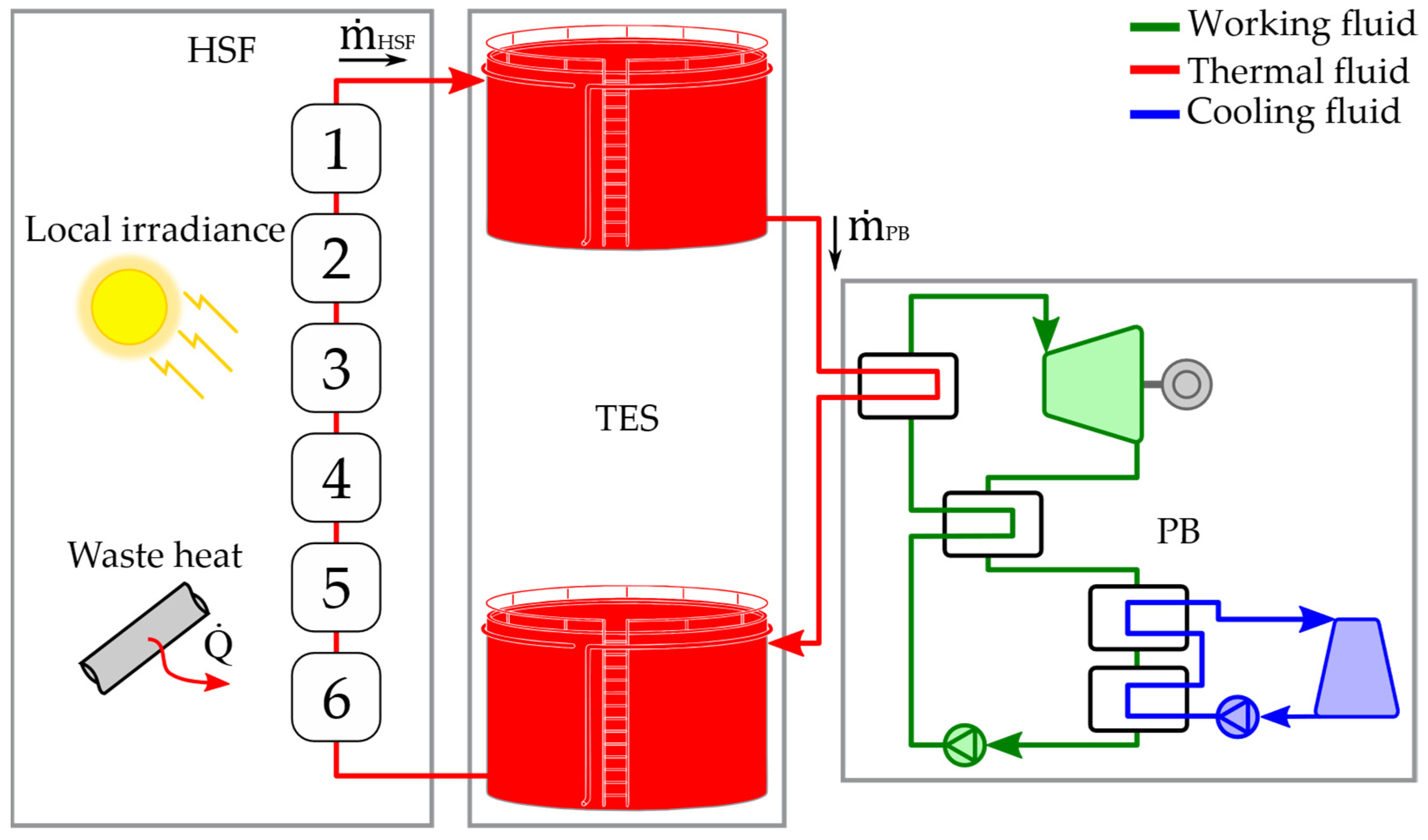
2. Hybrid Solar–Waste Heat Power System
3. Methodology
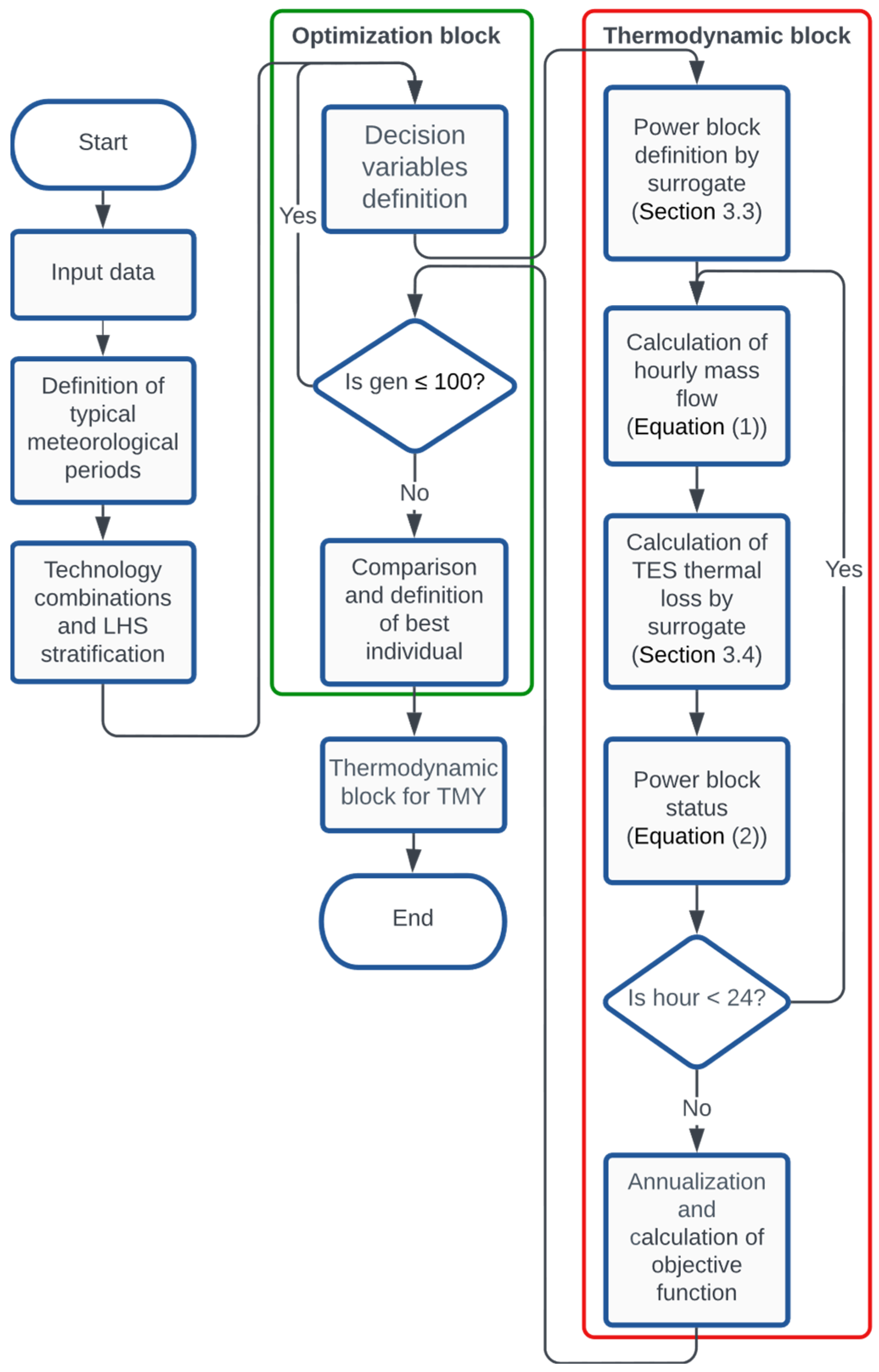
3.1. Optimization
Algorithm Logic
3.2. Hybrid Solar–Waste Heat Field
3.3. Power Block
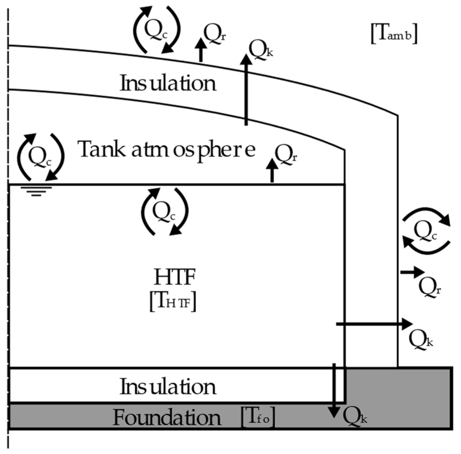
3.4. Storage Tank Heat Loss
3.5. Local Irradiance Data
3.6. Economic Model
4. Case Study
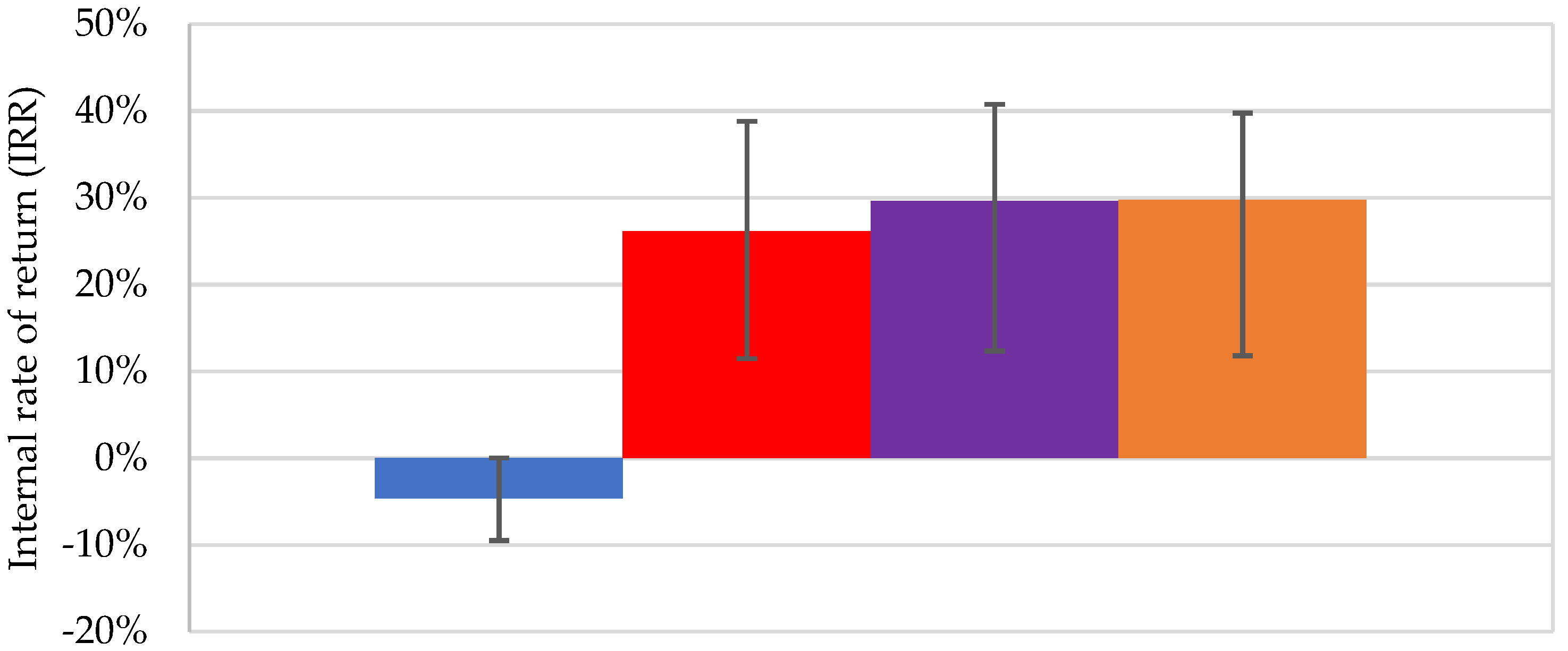
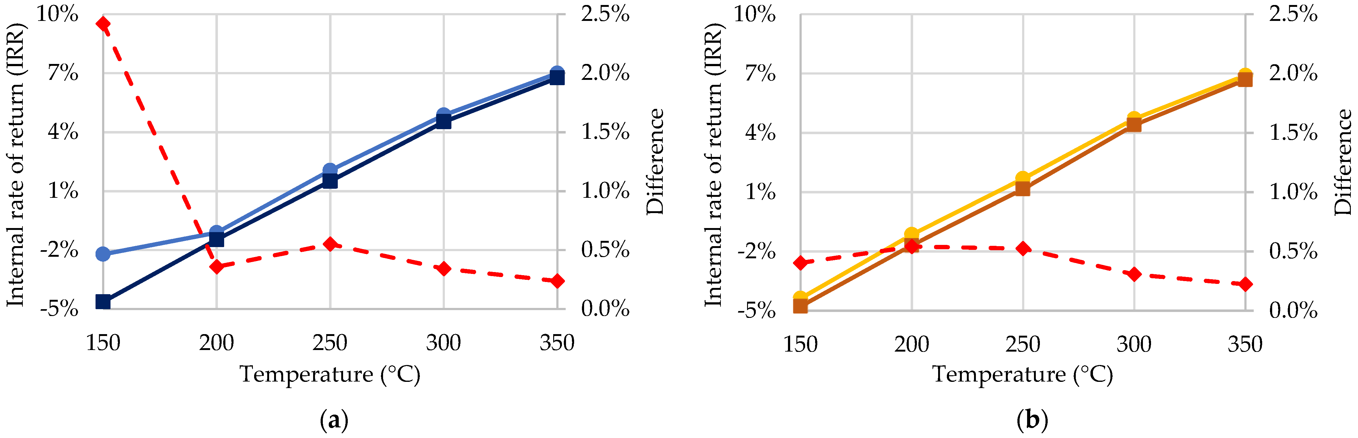
5. Results and Discussion
6. Conclusions
Author Contributions
Funding
Institutional Review Board Statement
Informed Consent Statement
Data Availability Statement
Acknowledgments
Conflicts of Interest
References
- Kalogirou, S.A. Solar Thermal Collectors and Applications. Prog. Energy Combust. Sci. 2004, 30, 231–295. [Google Scholar] [CrossRef]
- U. S. Energy Information Administration. International Energy Outlook 2019. Choice Rev. Online 2019, 85, 169.
- la Rocca, V.; Morale, M.; Peri, G.; Scaccianoce, G. A Solar Pond for Feeding a Thermoelectric Generator or an Organic Rankine Cycle System. Int. J. Heat Technol. 2017, 35, S435–S441. [Google Scholar] [CrossRef]
- Shamsi, H.; Boroushaki, M.; Geraei, H. Performance Evaluation and Optimization of Encapsulated Cascade PCM Thermal Storage. J. Energy Storage 2017, 11, 64–75. [Google Scholar] [CrossRef]
- Price, H.; Carpenter, S. The Potential for Low-Cost Electricity from Concentrating Solar Power Systems. In Proceedings of the 34th Intersociety Energy Conversion Engineering Conference, Vancouver, BC, Canada, 2–5 August 1999. [Google Scholar]
- Herrmann, U.; Kearney, D.W. Survey of Thermal Energy Storage for Parabolic Trough Power Plants. J. Sol. Energy Eng. 2002, 124, 145–152. [Google Scholar] [CrossRef] [Green Version]
- Duffie, J.A.; Beckman, W.A. Solar Engineering of Thermal Processes, 4th ed.; John Wiley & Sons, Inc.: Hoboken, NJ, USA, 2013; ISBN 9781118671603. [Google Scholar]
- Kalogirou, S.A. Solar Energy Engineering: Processes and Systems, 2nd ed.; Elsevier Inc.: Oxford, UK, 2014; ISBN 9780123972705. [Google Scholar]
- Mendecka, B.; Lombardi, L.; Gładysz, P.; Stanek, W. Exergo-Ecological Assessment of Waste to Energy Plants Supported by Solar Energy. Energies 2018, 11, 773. [Google Scholar] [CrossRef] [Green Version]
- Franchini, G.; Perdichizzi, A.; Ravelli, S.; Barigozzi, G. A Comparative Study between Parabolic Trough and Solar Tower Technologies in Solar Rankine Cycle and Integrated Solar Combined Cycle Plants. Sol. Energy 2013, 98, 302–314. [Google Scholar] [CrossRef]
- Rashid, K.; Safdarnejad, S.M.; Ellingwood, K.; Powell, K.M. Techno-Economic Evaluation of Different Hybridization Schemes for a Solar Thermal/Gas Power Plant. Energy 2019, 181, 91–106. [Google Scholar] [CrossRef]
- Chen, H.; Wu, Y.; Zeng, Y.; Xu, G.; Liu, W. Performance Analysis of a Solar-Aided Waste-to-Energy System Based on Steam Reheating. Appl. Therm. Eng. 2021, 185, 116445. [Google Scholar] [CrossRef]
- Arabkoohsar, A.; Sadi, M. Thermodynamics, Economic and Environmental Analyses of a Hybrid Waste–Solar Thermal Power Plant. J. Therm. Anal. Calorim. 2021, 144, 917–940. [Google Scholar] [CrossRef]
- Han, Y.; Sun, Y.; Wu, J. A Low-Cost and Efficient Solar/Coal Hybrid Power Generation Mode: Integration of Non-Concentrating Solar Energy and Air Preheating Process. Energy 2021, 235, 121367. [Google Scholar] [CrossRef]
- Behar, O.; Khellaf, A.; Mohammedi, K.; Ait-Kaci, S. A Review of Integrated Solar Combined Cycle System (ISCCS) with a Parabolic Trough Technology. Renew. Sustain. Energy Rev. 2014, 39, 223–250. [Google Scholar] [CrossRef]
- Brodrick, P.G.; Brandt, A.R.; Durlofsky, L.J. Operational Optimization of an Integrated Solar Combined Cycle under Practical Time-Dependent Constraints. Energy 2017, 141, 1569–1584. [Google Scholar] [CrossRef]
- Pantaleo, A.M.; Camporeale, S.M.; Sorrentino, A.; Miliozzi, A.; Shah, N.; Markides, C.N. Hybrid Solar-Biomass Combined Brayton/Organic Rankine-Cycle Plants Integrated with Thermal Storage: Techno-Economic Feasibility in Selected Mediterranean Areas. Renew. Energy 2020, 147, 2913–2931. [Google Scholar] [CrossRef]
- Alirahmi, S.M.; Rahmani Dabbagh, S.; Ahmadi, P.; Wongwises, S. Multi-Objective Design Optimization of a Multi-Generation Energy System Based on Geothermal and Solar Energy. Energy Convers. Manag. 2020, 205, 112426. [Google Scholar] [CrossRef]
- de Araújo Coutinho, D.P.; Rodrigues, J.A.M.M.; dos Santos, A.J.P.; de Almeida Semiao, V.S. Thermoeconomic Analysis and Optimization of a Hybrid Solar-Thermal Power Plant Using a Genetic Algorithm. Energy Convers. Manag. 2021, 247, 114669. [Google Scholar] [CrossRef]
- Elmorsy, L.; Morosuk, T.; Tsatsaronis, G. Exergy-Based Analysis and Optimization of an Integrated Solar Combined-Cycle Power Plant. Entropy 2020, 22, 655. [Google Scholar] [CrossRef]
- Rovira, A.; Abbas, R.; Muñoz, M.; Sebastián, A. Analysis of an Integrated Solar Combined Cycle with Recuperative Gas Turbine and Double Recuperative and Double Expansion Propane Cycle. Entropy 2020, 22, 476. [Google Scholar] [CrossRef] [Green Version]
- Witte, F.; Tuschy, I. TESPy: Thermal Engineering Systems in Python. J. Open Source Softw. 2020, 5, 2178. [Google Scholar] [CrossRef]
- Pedregosa, F.; Varoquaux, G.; Gramfort, A.; Michel, V.; Thirion, B.; Grisel, O.; Blondel, M.; Prettenhofer, P.; Weiss, R.; Dubourg, V.; et al. Scikit-Learn: Machine Learning in Python. J. Mach. Learn. Res. 2011, 12, 2825–2830. [Google Scholar]
- Bell, I.H.; Wronski, J.; Quoilin, S.; Lemort, V. Pure and Pseudo-Pure Fluid Thermophysical Property Evaluation and the Open-Source Thermophysical Property Library CoolProp. Ind. Eng. Chem. Res. 2014, 53, 2498–2508. [Google Scholar] [CrossRef] [PubMed] [Green Version]
- Sengupta, M.; Xie, Y.; Lopez, A.; Habte, A.; Maclaurin, G.; Shelby, J. The National Solar Radiation Data Base (NSRDB). Renew. Sustain. Energy Rev. 2018, 89, 51–60. [Google Scholar] [CrossRef]
- Benítez-Hidalgo, A.; Nebro, A.J.; García-Nieto, J.; Oregi, I.; del Ser, J. JMetalPy: A Python Framework for Multi-Objective Optimization with Metaheuristics. Swarm Evol. Comput. 2019, 51, 100598. [Google Scholar] [CrossRef] [Green Version]
- Bell, K.J. Shell-and-Tube Heat Exchangers. In The CRC Handbook of Thermal Engineering; Kreith, F., Ed.; CRC Press LLC: Boca Raton, FL, USA, 2000. [Google Scholar]
- Goswami, D.Y. Principles of Solar Engineering, 3rd ed.; CRC Press: Boca Raton, FL, USA, 2015; ISBN 9781466563797. [Google Scholar]
- Thomas, W.C.; Dawson, A.G.; Waksman, D.; Streed, E.R. Incident Angle Modifiers for Flat-Plate Solar Collectors: Analysis of Measurement and Calculation Procedures. J. Sol. Energy Eng. 1982, 104, 349–357. [Google Scholar] [CrossRef]
- Wagner, M.J. Results and Comparison from the SAM Linear Fresnel Technology Performance Model: Preprint. In Proceedings of the 2012 World Renewable Energy Forum, Denver, CO, USA, 13–17 May 2012. [Google Scholar]
- Wagner, M.J.; Zhu, G. A Direct-Steam Linear Fresnel Performance Model for NREL’s System Advisor Model. In Proceedings of the ASME 2012 6th International Conference on Energy Sustainability Collocated with the ASME 2012 10th International Conference on Fuel Cell Science, Engineering and Technology, San Diego, CA, USA, 23–26 July 2012. [Google Scholar]
- Price, H. A Parabolic Trough Solar Power Plant Simulation Model. In Proceedings of the ASME 2003 International Solar Energy Conference, Kohala Coast, HI, USA, 15–18 March 2003. [Google Scholar]
- Burkholder, F.; Kutscher, C. Heat Loss Testing of Schott’s 2008 PTR70 Parabolic Trough Receiver; National Renewable Energy Lab: Golden, CO, USA, 2009. [Google Scholar]
- Quoilin, S.; van den Broek, M.; Declaye, S.; Dewallef, P.; Lemort, V. Techno-Economic Survey of Organic Rankine Cycle (ORC) Systems. Renew. Sustain. Energy Rev. 2013, 22, 168–186. [Google Scholar] [CrossRef] [Green Version]
- Dincer, I.; Zamfirescu, C. Conventional Power Generating Systems. In Advanced Power Generation Systems; Elsevier: Amsterdam, The Netherlands, 2014; pp. 199–310. [Google Scholar]
- Moens, L.; Blake, D.M. Advanced Heat Transfer and Thermal Storage Fluids. In Proceedings of the ASME 2005 International Solar Energy Conference, Orlando, FL, USA, 6–12 August 2005. [Google Scholar]
- Jiménez-Arreola, M.; Wieland, C.; Romagnoli, A. Direct vs. Indirect Evaporation in Organic Rankine Cycle (ORC) Systems: A Comparison of the Dynamic Behavior for Waste Heat Recovery of Engine Exhaust. Appl. Energy 2019, 242, 439–452. [Google Scholar] [CrossRef]
- Vilasboas, I.F.; dos Santos, V.G.S.F.; Ribeiro, A.S.; da Silva, J.A.M. Surrogate Models Applied to Optimized Organic Rankine Cycles. Energies 2021, 14, 8456. [Google Scholar] [CrossRef]
- Zaversky, F.; García-Barberena, J.; Sánchez, M.; Astrain, D. Transient Molten Salt Two-Tank Thermal Storage Modeling for CSP Performance Simulations. Sol. Energy 2013, 93, 294–311. [Google Scholar] [CrossRef]
- Petrobras. N-550: Projeto de Isolamento Térmico a Alta Temperatura; CONTEC: Rio de Janeiro, Brazil, 1995. [Google Scholar]
- ABNT. NBR 7821: Tanques Soldados Para Armazenamento de Petróleo e Derivados; ABNT: Rio de Janeiro, Brazil, 1983. [Google Scholar]
- Araújo, A.K.A.; Medina, T.G.I. Analysis of the Effects of Climatic Conditions, Loading Level and Operating Temperature on the Heat Losses of Two-Tank Thermal Storage Systems in CSP. Sol. Energy 2018, 176, 358–369. [Google Scholar] [CrossRef]
- Pacheco, J.E.; Bradshaw, R.W.; Dawson, D.B.; De la Rosa, W.; Gilbert, R.; Goods, S.H.; Hale, M.J.; Jacobs, P.; Jones, S.; Kolb, G.; et al. Final Test and Evaluation Results from the Solar Two Project. Contract 2002, 294. [Google Scholar] [CrossRef] [Green Version]
- National Renewable Energy Laboratory. Andasol 1 CSP Project. Available online: https://solarpaces.nrel.gov/project/andasol-1 (accessed on 24 July 2021).
- Wilcox, S.; Marion, W. Users Manual for TMY3 Data Sets. 2008. Available online: https://www.nrel.gov/docs/fy08osti/43156.pdf (accessed on 4 April 2022).
- Bejan, A.; Tsatsaronis, G.; Moran, M. Thermal Design and Optimization, 1st ed.; John Wiley & Sons, Inc.: Hoboken, NJ, USA, 1995; ISBN 978-0-471-58467-4. [Google Scholar]
- Thermoflow Inc. Thermoflex; Thermoflow Inc.: Jacksonville, FL, USA, 2021. [Google Scholar]
- National Renewable Energy Laboratory. System Advisor Model 2021. Available online: https://sam.nrel.gov/ (accessed on 20 April 2022).
- Industrial Solar. Industrial Solar Fresnel Collector LF-11 Datasheet 1–3; Industrial Solar: Freiburg, Germany, 2020. [Google Scholar]
- Banco Central do Brasil. Focus-Market Readout. 2022. Available online: https://www.bcb.gov.br/en/publications/focusmarketreadout (accessed on 5 April 2022).


| Variable | Description | Type | Lower Bound | Upper Bound |
|---|---|---|---|---|
| Structure Decision Variables | Binary | 0 | 1 | |
| Aperture or Heat Exchanger Areas | Continuous | 0 m | 1 × 10⁶ m | |
| Heat Transfer Rate to PB | Continuous | 100 kW | 50,000 kW | |
| PB Inlet Temperature | Continuous | 106 °C | 350 °C | |
| PB Outlet Temperature | Continuous | 96 °C | 340 °C | |
| TES Storage Capacity | Continuous | 0 h | 12 h |
| Variable | Type | Lower Bound | Upper Bound |
|---|---|---|---|
| Evaporation Pressure | Decision Variable | 4.01325 bar | 42 bar |
| Condensation Pressure | Decision Variable | 1.01325 bar | Working Fluid Critical Pressure |
| Turbine Inlet Temperature | Decision Variable | Condensation Temperature | Source Inlet Temperature |
| Recuperator Outlet Temperature at Cold Side | Decision Variable | Condensation Temperature | Source Outlet Temperature |
| Evaporator Plate Width | Decision Variable | 0.3048 m | 4.572 m |
| Condenser Plate Width | Decision Variable | 0.3048 m | 4.572 m |
| Recuperator Plate Width | Decision Variable | 0.3048 m | 4.572 m |
| Evaporator Working Fluid Velocity | Decision Variable | 0.2 m/s | 2.0 m/s |
| Condenser Working Fluid Velocity | Decision Variable | 0.2 m/s | 2.0 m/s |
| Recuperator Working Fluid Velocity | Decision Variable | 0.2 m/s | 2.0 m/s |
| Pinch Point Temperature Difference | Constraint | 4 °C | - |
| Turbine Pressure Difference | Constraint | 3 bar | - |
| Quality During Expansion | Constraint | 0.8 | - |
| Heat Exchanger Pressure Drop | Constraint | 0 | 1.8 bar |
| Variable | Description | Value | Reference |
|---|---|---|---|
| HTF Costs | 20% | [48] | |
| Equipment Installation Costs | 30% | [46] | |
| Piping Costs | 20% | [46] | |
| Instrumentation and Control Costs | 30% | [46] | |
| Electrical Equipment Costs | 10% | [46] | |
| Civil, Structural and Architectural Costs | 10% | [46] | |
| Service Facilities Costs | 40% | [46] | |
| Engineering and Supervisor Costs | 10% | [46] | |
| Contingences | 10% | [46] |
| Collector Type | Manufacturer | Model | Maximum Operating Temperature | Reference |
|---|---|---|---|---|
| Flat Plate | SolarTEK | ST400 | 208 °C | [48] |
| Evacuated Tube | Kingspan Solar Inc. | Thermomax DF100-30 | 300 °C | [48] |
| Linear Fresnel | Industrial Solar | LF-11 | 400 °C | [49] |
| Parabolic Trough | SkyFuel (Reflector) Solel (Receiver) | SkyTrough (Reflector) UVAC3 (Receiver) | 560 °C | [48] |
Publisher’s Note: MDPI stays neutral with regard to jurisdictional claims in published maps and institutional affiliations. |
© 2022 by the authors. Licensee MDPI, Basel, Switzerland. This article is an open access article distributed under the terms and conditions of the Creative Commons Attribution (CC BY) license (https://creativecommons.org/licenses/by/4.0/).
Share and Cite
Vilasboas, I.F.; dos Santos, V.G.S.F.; de Morais, V.O.B.; Ribeiro, A.S., Jr.; da Silva, J.A.M. AERES: Thermodynamic and Economic Optimization Software for Hybrid Solar–Waste Heat Systems. Energies 2022, 15, 4284. https://doi.org/10.3390/en15124284
Vilasboas IF, dos Santos VGSF, de Morais VOB, Ribeiro AS Jr., da Silva JAM. AERES: Thermodynamic and Economic Optimization Software for Hybrid Solar–Waste Heat Systems. Energies. 2022; 15(12):4284. https://doi.org/10.3390/en15124284
Chicago/Turabian StyleVilasboas, Icaro Figueiredo, Victor Gabriel Sousa Fagundes dos Santos, Vinicius Oliveira Braz de Morais, Armando Sá Ribeiro, Jr., and Julio Augusto Mendes da Silva. 2022. "AERES: Thermodynamic and Economic Optimization Software for Hybrid Solar–Waste Heat Systems" Energies 15, no. 12: 4284. https://doi.org/10.3390/en15124284
APA StyleVilasboas, I. F., dos Santos, V. G. S. F., de Morais, V. O. B., Ribeiro, A. S., Jr., & da Silva, J. A. M. (2022). AERES: Thermodynamic and Economic Optimization Software for Hybrid Solar–Waste Heat Systems. Energies, 15(12), 4284. https://doi.org/10.3390/en15124284