A Modified SOGI-PLL with Adjustable Refiltering for Improved Stability and Reduced Response Time

Abstract

The controls of most power electronic inverters connected to an electrical power system (EPS) rely on the precise determination of the voltage magnitude, frequency, and phase angle at the point of common coupling. One of the most widely used approaches for measuring these quantities is the phase-locked loop (PLL); however, the precision of this measurement is affected during transients in the EPS and is a function of the type of event and the architecture of the PLL. PLLs based on the second-order generalized integrator (SOGI) are widely used in power converter synchronization, offering an adaptive or fixed-parameter prefilter with low-pass and band-pass characteristics. This article proposes a variant of the SOGI-PLL that offers improved stability and a faster response time. This is accomplished by decoupling the effect of the SOGI’s gains and adding feedback. The modification is carried out in the state space model of the SOGI. Manipulating the attenuation moves the poles of the SOGI to improve the stability. The performance of the proposed PLL is verified and validated under the processor-in-the-loop (PIL) approach.

1. Introduction

In recent years, the integration of distributed generation (DG) units to the electrical power system (EPS) has increased. A fundamental aspect of a correct interconnection is the DG inverter synchronization algorithm. For a stable and reliable operation, this algorithm must ensure that the inverter voltage waveform synchronizes with the main voltages, even under disturbances within the EPS [1,2,3,4,5]. The most widely used synchronization approach is the phase-locked loop (PLL). However, the operation of the PLL is compromised when the network voltage and current contain harmonics and when the network is subject to faults and disturbances [2,6,7,8,9]. No matter how reliable the transmission and distribution system is, unbalanced voltages and harmonic distortions at the PLL input are unavoidable [2,9].

It must be taken into account that the grid frequency can show considerable fluctuations during transients and faults in power systems with high DG penetration [10]. This implies that the synchronization system must be insensitive to network frequency variations [11]. On the other hand, large voltage sags and other transient events can cause incorrect transient frequency measurements in the PLL [12,13,14,15,16]. PLLs that include non-adaptive strategies, as well as notch filters, present problems when the EPS frequency deviates from its nominal value. The problem can become serious in the presence of large deviations from the nominal frequency of the EPS, particularly under severe asymmetrical voltage sags or faults [5,12].

Phase-to-ground faults constitute up to 95% of the faults that occur in the EPS [17]. This type of fault causes voltage sags in the distribution and transmission systems. When this and other types of faults are cleared, transients appear that range from nominal frequency levels to levels the tens of kHz [18]. On the other hand, in general, a harmonic of order h present in the input signal becomes a harmonic of order $(h-1)$ (if it is a positive-sequence harmonic) or $(h+1)$ (if it is a negative-sequence harmonic) in the $dq$ frame [19]. Therefore, the fundamental negative-sequence component causing the asymmetry in the grid voltage becomes the second harmonic ripple in the $dq$ frame, and the displacement dc becomes the fundamental component. Consequently, the loop filter must be able to attenuate the second harmonic and the fundamental component. Eliminating the fundamental negative-sequence component without compromising the dynamic performance remains a demanding task in PLL design [20]. To achieve this, the bandwidth of the PLL must be drastically reduced [2,12,21]. However, with low bandwidth, the transient response becomes slow [15,22,23,24]. The main challenge associated with PLLs is to achieve a fast dynamic response without compromising the harmonic rejection capability while ensuring that disturbances in the electrical network do not drive the PLL to instability and the loss of synchronism [24,25,26,27]. The filter bandwidth should be a trade-off between filtering performance, time response, and stability [2,9,22].

One of the most frequently used synchronization algorithms is the second-order generalized integrator phase-locked loop (SOGI-PLL) due to its simplicity, low computational cost, and independence from network frequency, and because it avoids filtering delays [28,29,30]. In this paper, a modification of the SOGI-PLL architecture is proposed; the modification improves the stability of the quadrature signal generator (QSG) stage and increases the bandwidth of the PLL structure, achieving a fast response of the PLL as a whole, without sacrificing the harmonic rejection capability of the traditional SOGI-PLL. This is achieved by decoupling the effect of the single SOGI-QSG gain, allowing a second QSG gain to be introduced, and adding feedback from the band-pass filter output signal to the QSG input. The new QSG gain permits the manipulation of the extra attenuation while moving the QSG poles to improve stability. The decoupling of the SOGI gain is carried out by converting the transfer function of the SOGI-QSG [6,28] block diagram to a model in the state space in the controllable canonical form, since in the state space there is direct access to the sections of the QSG algorithm where gains appear. A functional structure of the ARF-SOGI-QSG is reported in the state space and also in block form. The proposed structure is a PLL with adjustable re-filtering based on a second-order generalized integrator, abbreviated to ARF-SOGI-PLL from now on.

The paper is organized as follows: Section 2.1 describes the PLL performance evaluation criteria, Section 2.2 summarizes the main characteristics of the SOGI-PLL and develops the structure of the modified SOGI-QSG, whose characteristics are further discussed in Section 2.3 and Section 2.4. In Section 2.5, the proposed ARF-SOGI-PLL structure is presented; its performance is assessed for different disturbances in the electrical system in Section 3. The computational resources and execution times of the tested PLLs are also compared. The conclusions are presented in Section 4.

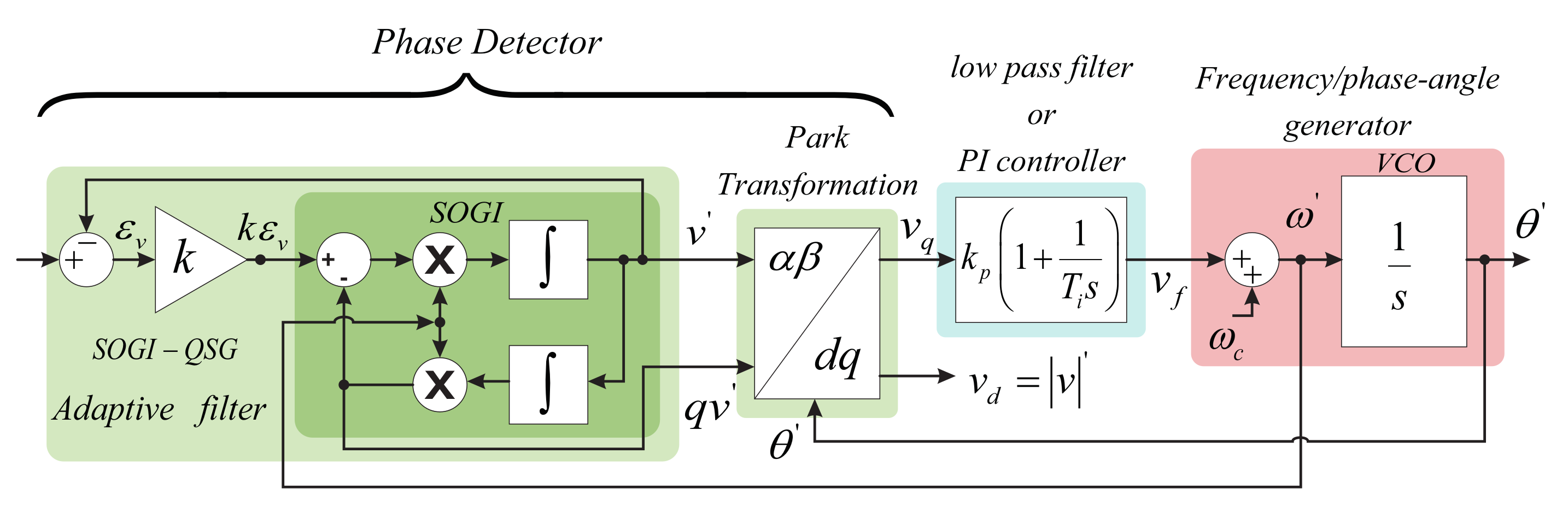
2. Development of the Improved PLL

In this section, an improved SOGI-PLL is proposed. The desirable improvements in performance are listed in the following section. The key characteristics of the traditional SOGI-PLL are reviewed in order to motivate the proposed modifications.

2.1. The PLL Performance Evaluation Criteria

The total harmonic distortion (THD) of the unit vectors and the synchronization time will be used as the criteria for assessing the performance of the PLL. A THD of less than 1% will be deemed as acceptable. The unit vectors are the evaluation of the sine and cosine functions of the angle calculated by the PLL. These vectors must be in synchrony with the main voltages but without harmonic contamination, since the reference signals for the control of the inverter are obtained from the angle calculated by the PLL.

Very short synchronization times generally imply a degradation in the quality of the unit vectors. On the other hand, high-frequency deviations lead to longer synchronization times or a failed re-synchronization. In both cases, the extraction of the frequency from the network will be incorrect during the PLL transient. Therefore, there is a need to improve the PLL response in two regards: increase the speed with which the correct value of the frequency is reported (without degrading the quality of the unit vectors), and reduce the error in the reported frequency during the PLL transient [27].

The disconnection times of the converter in case of voltage variations are established in the IEEE 1547, IEC61727, and VDE0126-1-1 standards [12,31,32]. Similarly, the rules applied in the case of frequency deviations and the allowable ranges are discussed in [12,31,32]. The IEEE 1547 standard states that for disturbances for which the system frequency remains between 58.8 Hz and 61.2 Hz, the converter must remain operational and must continue to provide active power. The low-frequency ride-through period is 299 s in the range $57.0\le f\le 58.8$ Hz, while the high-frequency ride-through range is $61.2<f\le 61.8$ Hz. Within these ranges and periods, the converter must not trip and must continue to provide active power. For a frequency deviation greater than 3.5 Hz, the converter is disconnected after a period of 0.16 s. Therefore, a PLL must avoid erroneously reporting a deviation of this magnitude for more than 0.16 s.

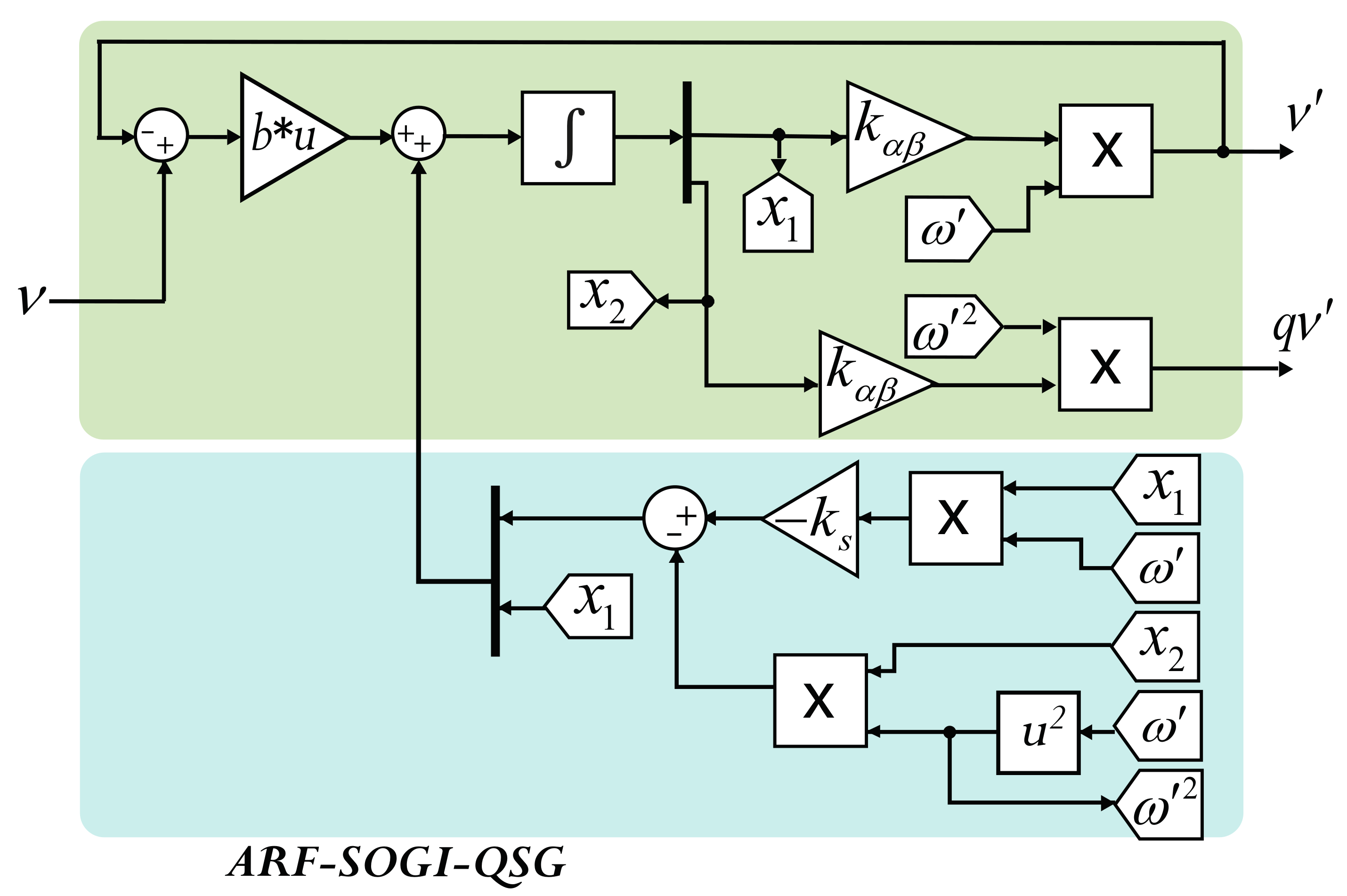
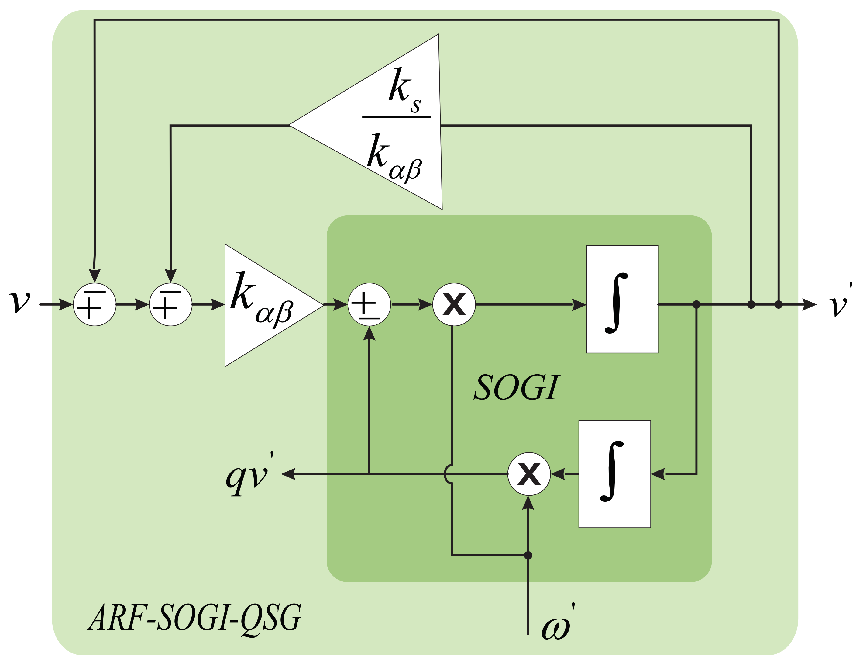
2.2. Proposed ARF-SOGI-QSG Structure

The PLL proposed in this article is based on the modification of the SOGI-PLL, whose structure is shown in Figure 1. The SOGI-PLL is based on a QSG and generally consists of three stages: a phase detector, a controller (also called loop filter), and a frequency and phase-angle generator. The phase detector is constructed with a QSG and a Park transformation stage. The QSG is built around a SOGI, which helps in providing adaptative filter characteristics to the QSG. Therefore the complete structure of the SOGI-PLL contains, in addition to a loop filter, an adaptative pre-filtering stage, contributing to the improvement of the harmonic rejection and to the SOGI-PLL’s tolerance to frequency changes. The main characteristics of the SOGI-PLL can be summarized as follows:

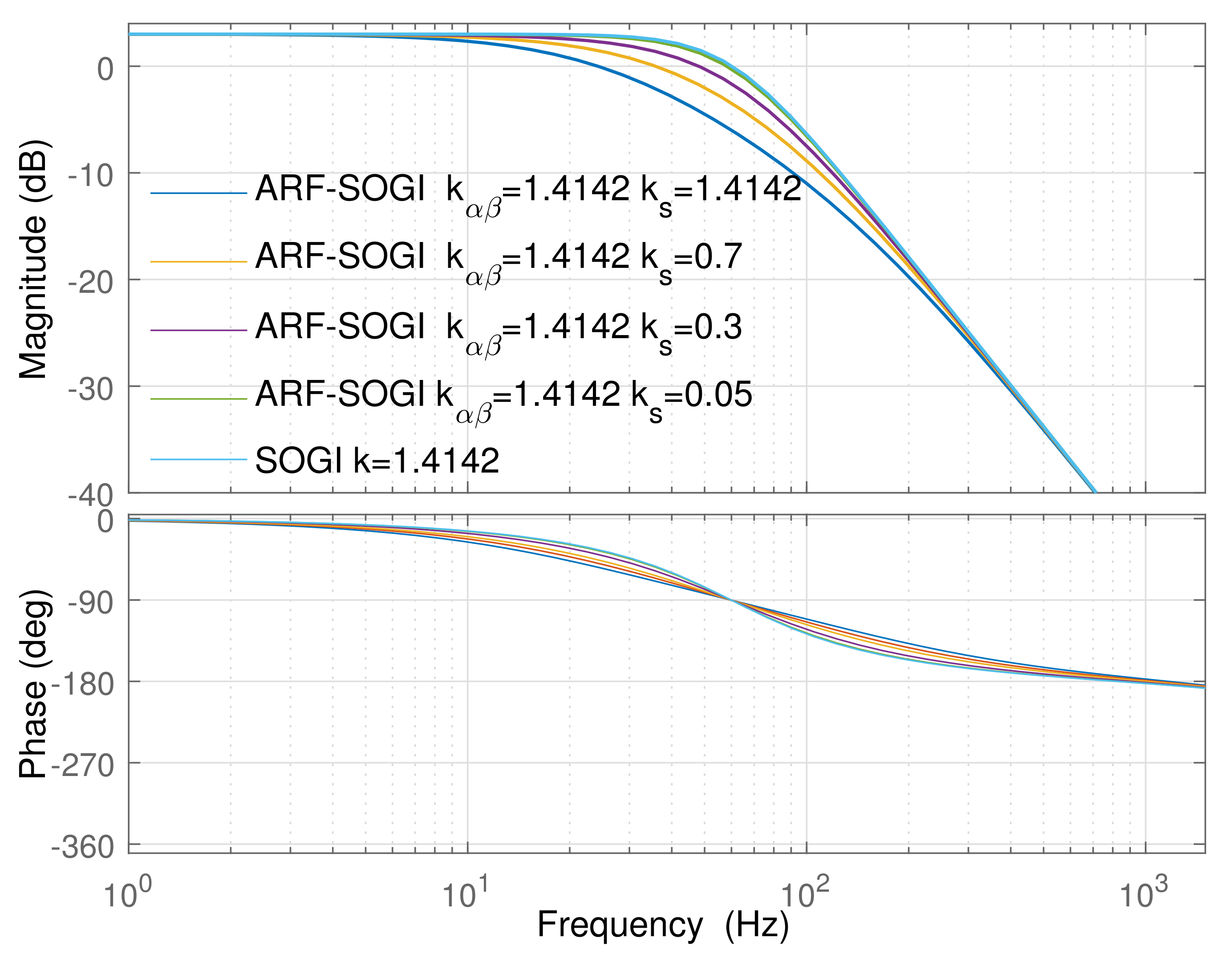
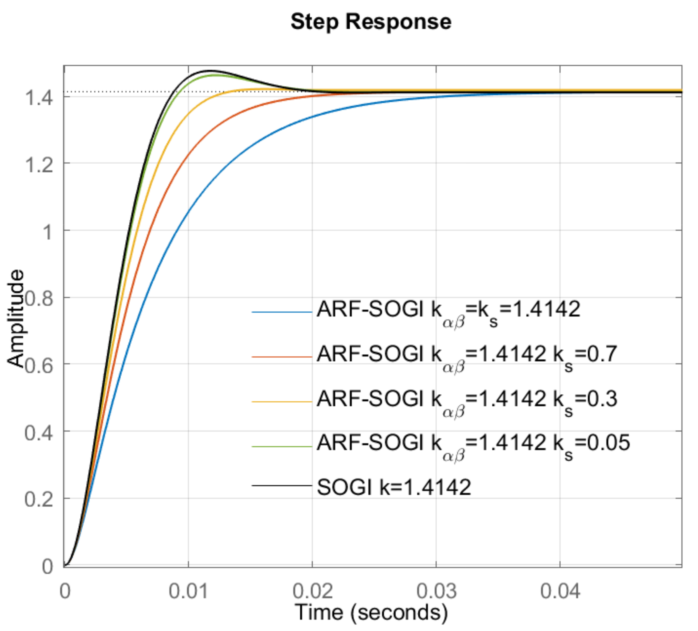
• The value of the single gain k of the adaptive prefilter affects all the characteristics of the SOGI-QSG;
• The magnitude of the line voltage is calculated by the Park transformation and reported as $V_d$, as shown in Figure 1;
• The frequency calculated by the PLL is fed back to the SOGI block;
• The angle is calculated by the integrator or VCO and fed back to the Park transformation block.

The transfer functions that characterize the SOGI-QSG and the prefiltering process are given by:

$$SOGI\left(s\right)=\frac{v^{\prime }}{k{\epsilon }_v}\left(s\right)=\frac{{\omega }^{\prime }s}{s^2+{\omega }^{\prime 2}}$$

(1)

$$D\left(s\right)=\frac{v^{\prime }}{v}\left(s\right)=\frac{k{\omega }^{\prime }s}{s^2+k{\omega }^{\prime }s+{\omega }^{\prime 2}}$$

(2)

$$Q\left(s\right)=\frac{q{v}^{\prime }}{v}\left(s\right)=\frac{k{\omega }^{\prime 2}}{s^2+k{\omega }^{\prime }s+{\omega }^{\prime 2}}.$$

(3)

The transfer Functions (2) and (3) are obtained from the transfer Function (1) of the SOGI. These transfer functions show that the bandwidth of the adaptive filter based on SOGI is not a function of the center frequency and that it only depends on the gain k [12]. Moreover, it is clear that the single gain k directly impacts three parts of the algorithm. This suggests a modification of the SOGI-QSG structure, consisting in distributing the influence of the gain over each prefilter stage. To do this, the model is represented in the state space. The controllable canonical form of Equation (2), which corresponds to the band-pass filter, is given by:

$$\underset{\dot{\mathbf{x}}}{\underbrace{\left[\begin{array}{c}{\dot{x}}_1\\ {\dot{x}}_2\end{array}\right]}}=\underset{\mathbf{A}}{\underbrace{\left[\begin{array}{cc}-k{\omega }^{\prime }& -{\omega }^{\prime 2}\\ 1& 0\end{array}\right]}}\underset{\mathbf{x}}{\underbrace{\left[\begin{array}{c}{x}_1\\ x_2\end{array}\right]}}+\underset{\mathbf{b}}{\underbrace{\left[\begin{array}{c}1\\ 0\end{array}\right]}}v$$

(4)

$$y=\underset{\mathbf{c}}{\underbrace{\left[\begin{array}{cc}k{\omega }^{\prime }& 0\end{array}\right]}}\left[\begin{array}{c}{x}_1\\ x_2\end{array}\right],$$

(5)

while the corresponding expressions for the low-pass filter (Equation (3)) are:

$$\left[\begin{array}{c}{\dot{x}}_1\\ {\dot{x}}_2\end{array}\right]=\left[\begin{array}{cc}-k{\omega }^{\prime }& -{\omega }^{\prime 2}\\ 1& 0\end{array}\right]\left[\begin{array}{c}{x}_1\\ x_2\end{array}\right]+\left[\begin{array}{c}1\\ 0\end{array}\right]v$$

(6)

$$y=\left[\begin{array}{cc}0& k{\omega }^{{}^{\prime }2}\end{array}\right]\left[\begin{array}{c}{x}_1\\ x_2\end{array}\right].$$

(7)

The proposed SOGI-QSG form is shown in Figure 2. The new structure is based on Equations (4) to (7). Figure 2 shows, in the inferior part, the multiplication of matrix $\mathbf{A}$ by the vector of states $\dot{\mathbf{x}}$, and in the upper part (which contains the output signals), the multiplication of only the state of interest with the part of the vector $\mathbf{c}$ that corresponds to both the band-pass filter and the output low-pass filter $\left(y\right)$. The use of this structure makes it possible to modify the value of the gains independently.

It is possible to add a negative feedback loop from the $v^{\prime }$ output of the SOGI band-pass filter to its input. This extra closed loop provides a higher attenuation in the outputs $v^{\prime }$ and $q{v}^{\prime }$, in contrast to the traditional adaptative filter.

The model in the state space allows access to the gains in the different sections in the QSG, and with this, the performance of the ARF-SOGI-QSG can be improved. With the proposed method arises the possibility to use three different gains. However, finding the values of the gains is not a trivial task. The next remarks must be taken into account:

• Since the gain $k_s$ in Figure 2 can be adjusted in value without unbalancing the magnitude of the responses $v^{\prime }$ and $q{v}^{\prime }$, the change in the value of this gain does not affect the orthogonality of the two signals;
• Using different gain values at the outputs $v^{\prime }$ and $q{v}^{\prime }$ of the filtering could only be possible with very slight differences (of the order of ${10}^{-3}$). Greater differences cause a different attenuation in the magnitude of signals $v^{\prime }$ and $q{v}^{\prime }$, which can produce imbalances and, therefore, oscillations at the PLL output (at twice the fundamental frequency of the input signal). Hence, it is recommended that these two gains from the ARF-SOGI-QSG output are equal, and from now on, the single gain is called $k_{\alpha \beta }$, as seen in Figure 2;
• If $k_s=k_{\alpha \beta }$, the attenuation suffered by the 30 Hz and 120 Hz signals is approximately 3.9 dB; this is an advantage over the traditional SOGI, but the cost is an attenuation of approximately 6 dB in the fundamental frequency signal. However, adjustment of the gain $k_s$ corrects this attenuation, as discussed in Section 3.5;
• The smaller the value of $k_s$, the closer the ARF-SOGI-QSG is to the traditional SOGI-QSG;
• The greater the $k_s$, the greater the attenuation suffered by the fundamental frequency of the voltage signal.

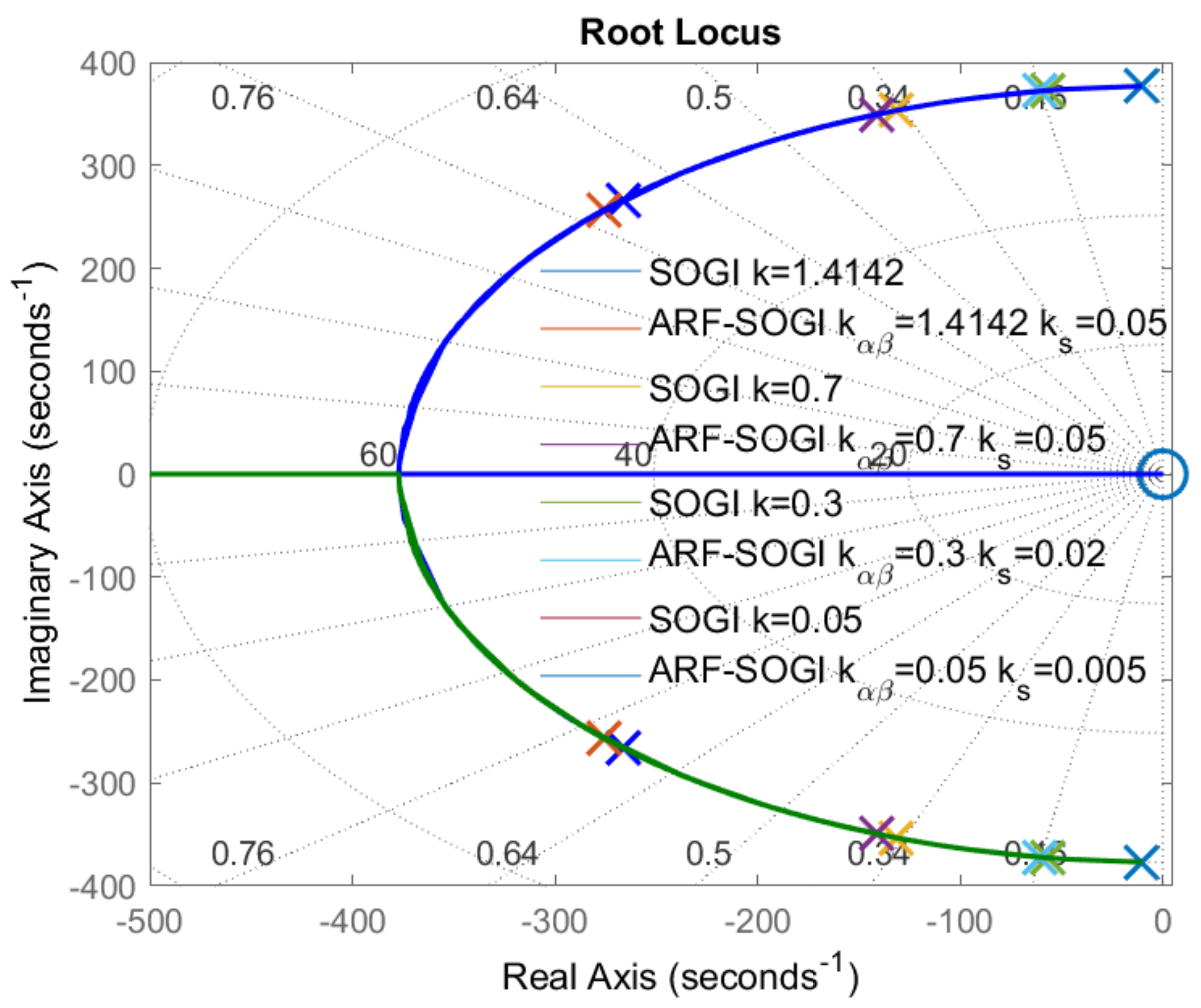
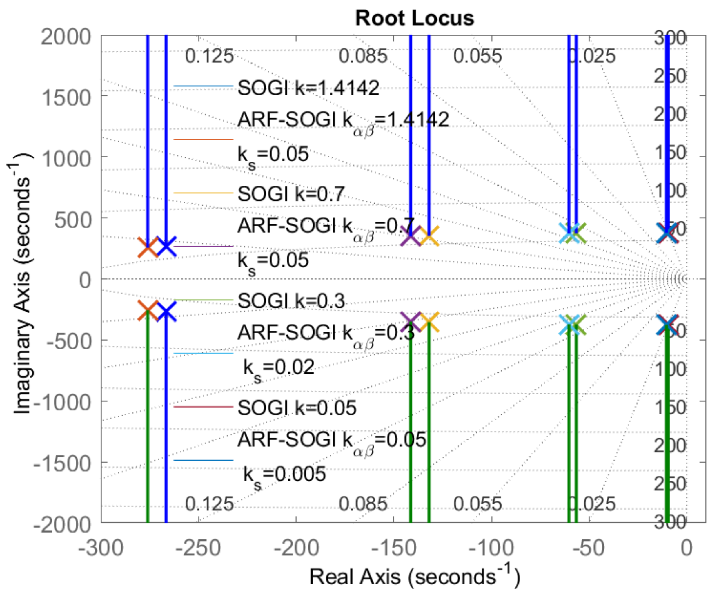
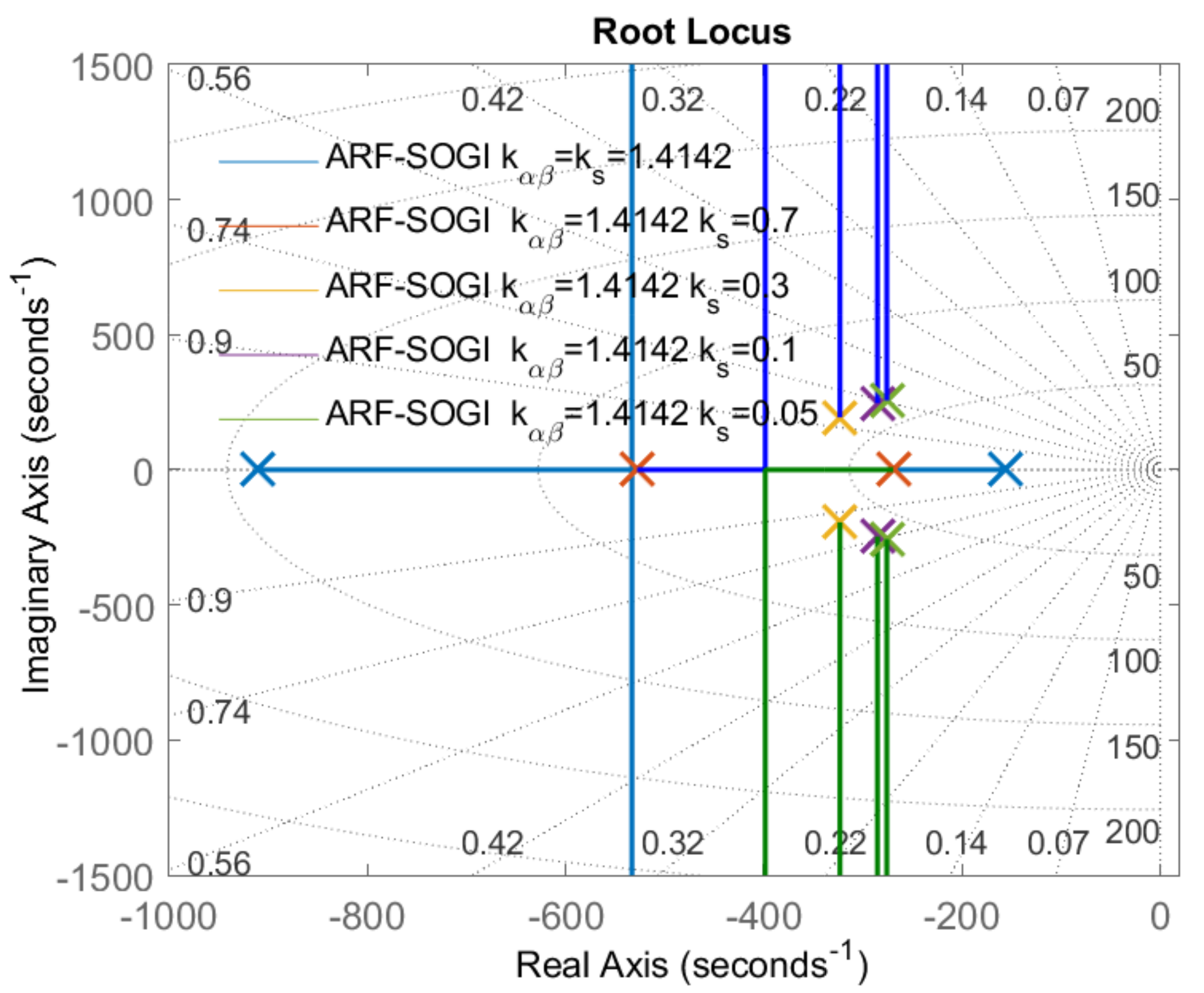
2.3. ARF-SOGI-QSG Transfer Functions

The form of the proposed architecture in the frequency domain is shown in Figure 3.

The transfer functions of the ARF-SOGI-QSG can be obtained from the diagram in Figure 3, and is given by:

$$SOG{I}_m\left(s\right)=\frac{v^{\prime }}{{\epsilon }_v}=\frac{k_{\alpha \beta }{\omega }^{\prime }s}{s^2+{\omega }^{\prime 2}}$$

(8)

The transfer function of the signal $v^{\prime }$ band-pass characteristic is given by:

$$D_m\left(s\right)=\frac{v^{\prime }}{v}\left(s\right)=\frac{k_{\alpha \beta }{\omega }^{\prime }s}{s^2+{\omega }^{\prime }s\left(k_s+k_{\alpha \beta }\right)+{\omega }^{\prime 2}}$$

(9)

The transfer function of the quadrature signal $q{v}^{\prime }$ low-pass characteristic is given by:

$$Q_m\left(s\right)=\frac{q{v}^{\prime }}{v}\left(s\right)=\frac{k_{\alpha \beta }{\omega }^{\prime 2}}{s^2+{\omega }^{\prime }s\left(k_s+k_{\alpha \beta }\right)+{\omega }^{\prime 2}}$$

(10)

It is clearly seen, from the transfer functions (9) and (10), that the smaller the $k_s$, the closer the transfer functions are to the original transfer functions (Equations (2) and (3)) from the SOGI-QSG.

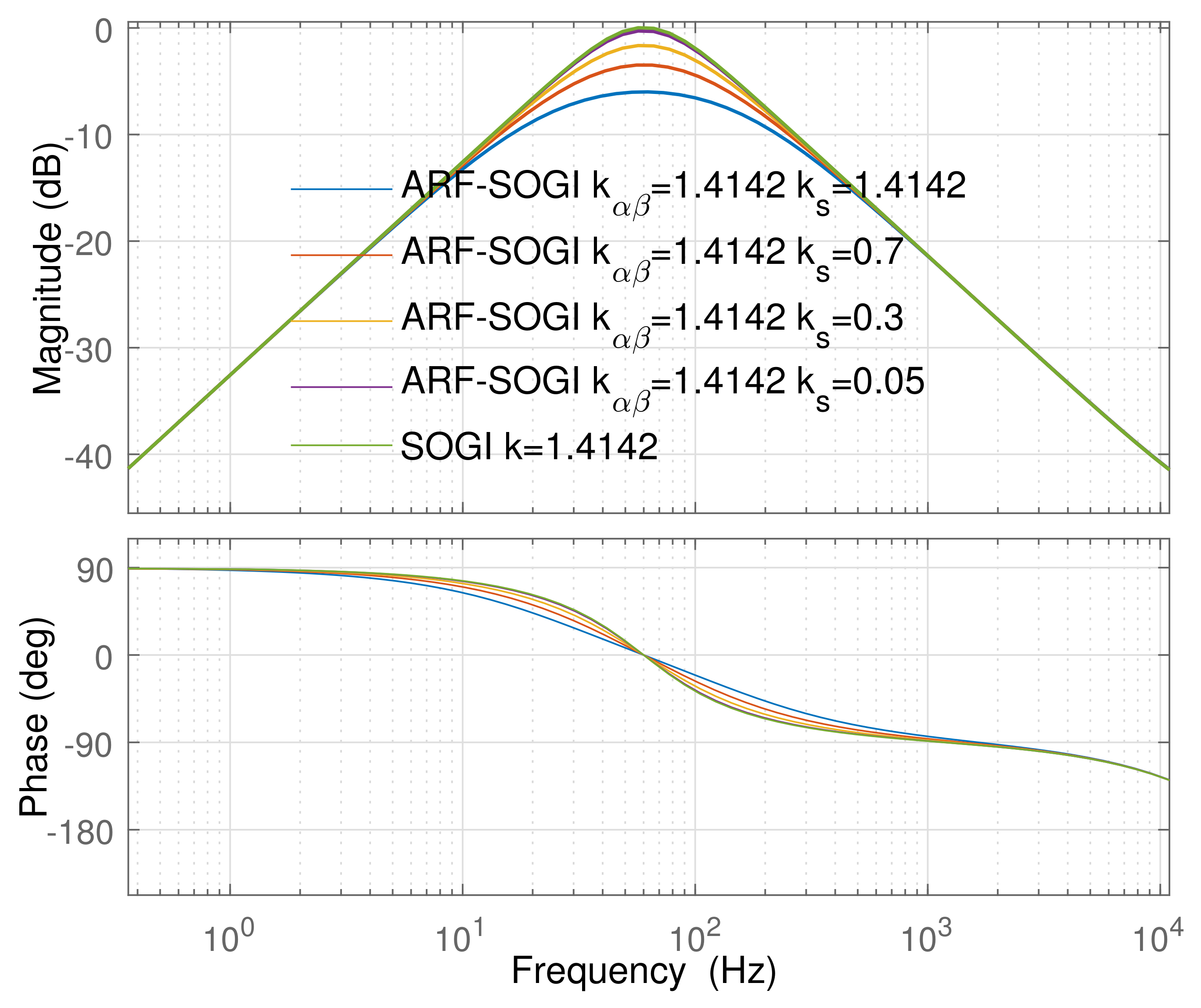
2.4. Comparative Analysis of SOGI-QSG and ARF-SOGI-QSG

Figure 4 and Figure 5 compare the Bode diagrams corresponding to the transfer functions (2) and (3) and the proposed ARF-SOGI-QSG. The diagrams confirm the remarks of the previous section: the types of filtering implicit in the SOGI are preserved in the proposed modification, but a greater attenuation is seen within a range of approximately $\left[\frac{1}{2}f,2f\right]$. Such extra attenuation is more significant at the fundamental frequency. It is also observed that the attenuation in this range can be controlled by varying the gain $k_s$. Likewise, the orthogonality characteristic is preserved, and it is seen that the extra attenuation reported by the ARF-SOGI-QSG comes from the modification made in the denominator of the transfer functions.

Regarding the stability of the SOGI-QSG and the ARF-SOGI-QSG, Figure 6 and Figure 7 show the effect of different values of k, $k_s$, and $k_{\alpha \beta }$. When the bandwidth is reduced, the systems approximate the stability limit. Figure 6 and Figure 7 show one of the advantages of the ARF-SOGI-QSG, namely, the feasibility of tuning the filter gains ($k_s$, $k_{\alpha \beta }$) independently. If $k_{\alpha \beta }$ is set higher than $k_s$, the position of the poles is moved to the left, compared to the poles of the SOGI, moving away from the instability region with the option to have the bandwidth reduced only slightly.

It is worth noticing that as stability is improved, the frequencies of interest are attenuated while the bandwidth is reduced; however, it is possible to find a combination that is acceptable, where $k_s$ is not so small with respect to $k_{\alpha \beta }$. It is recommended to select $k_s$ and $k_{\alpha \beta }$ values so that, in the unit-step test, the ARF-SOGI-QSG filters do not overshoot, in a similar manner to that of a critically damped system or to an over-damped system. This prevents large transient overshoots during phase jump disturbances and frequency deviations. As seen in Figure 8 and Figure 9, when the value of $k_s$ tends to the value of $k_{\alpha \beta }$, the ARF-SOGI-QSG poles are real and lie in the left half-plane, but one of the poles is approaching the imaginary axis. This implies that the system is over-damped (for instance, look at the poles when $k_s=k_{\alpha \beta }=1.4142$).

An improved unit-step response is another advantage of the ARF-SOGI-QSG. In Figure 10, it can be seen that the unit-step response with $k=1.4142$ in the traditional SOGI exhibits an overshoot before stabilizing. The same figure (Figure 10) shows how, in the ARF-SOGI, it is possible to eliminate that overshoot by tuning $k_{\alpha \beta }=1.4142,k_s=0.3$, achieving the steady state earlier than the traditional SOGI-QSG. As mentioned before, the closer $k_s$ is to $k_{\alpha \beta }$, the more the attenuation of the fundamental frequency is increased, which is undesirable. However, in Figure 10, it can be seen how $k_s$, in this case, can be adjusted to a value lower than $k_s=0.3$ without a significant overshoot. This improves the stability of the system, reduces the level of attenuation in the fundamental, and speeds up the response. A similar behavior occurs in the output corresponding to the band-pass effect of the ARF-SOGI-QSG.

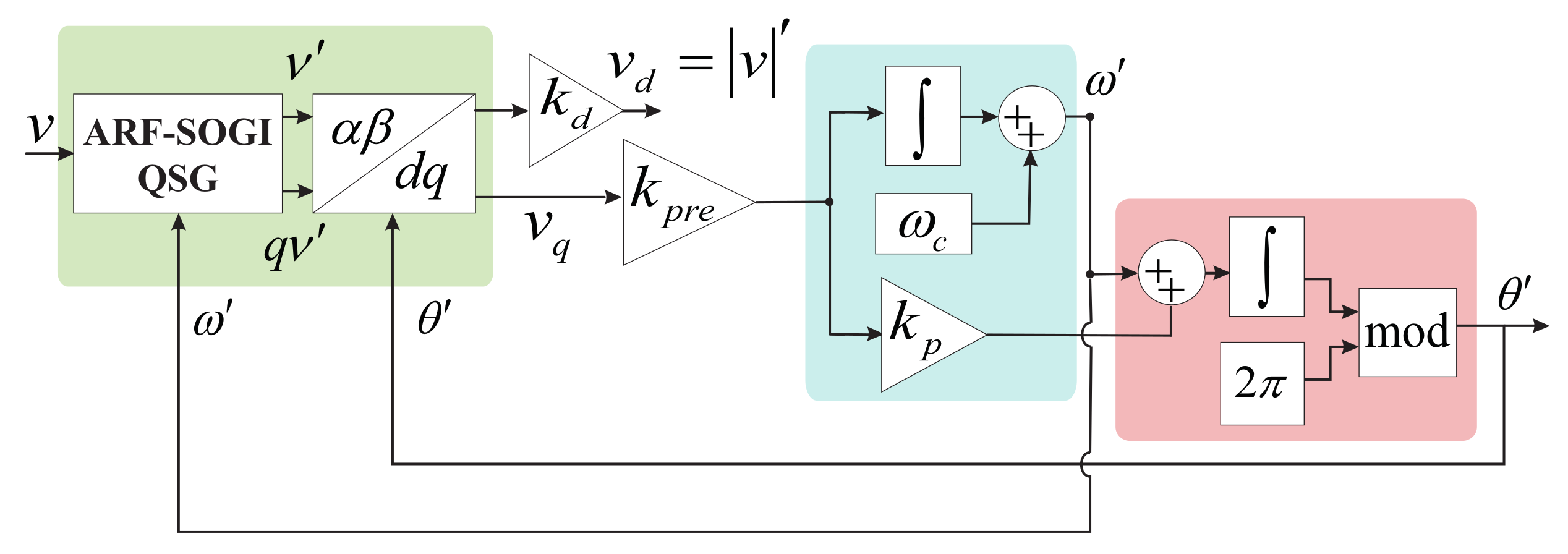
2.5. The ARF-SOGI-PLL

To implement a PLL based on ARF-SOGI-QSG, the architecture of an SRF-PLL is added to the ARF-SOGI-QSG, as shown in Figure 11.

Since the ARF-SOGI-QSG is more robust than the traditional SOGI-QSG, it is possible to increase the bandwidth of the loop filter. This is accomplished by increasing the value of the $k_p$ and $k_i$ gains in the PLL, or by selecting a large value for $k_i$ under a standard design method for the selection of parameters [21]. In the proposed PLL, the multiplication of $k_{pre}$ by the loop PI filter gains increases the bandwidth of the PLL. The PLL based on the ARF-SOGI is composed of the following stages:

• The modified SOGI-QSG block (ARF-SOGI-QSG);
• The $k_{pre}$ gain, which compensates for the extra attenuation caused by the ARF-SOGI and increases the loop bandwidth of the SRF-PLL embedded in the PLL;
• An SRF-PLL with frequency extraction using an integral controller.

To assess the performance of the proposed PLL, its response is compared with that of the traditional SOGI-PLL and the SOGI-PLL with an estimated frequency extracted from the PI controller integrator output [5] (referred to as SOGI-PLL-EFI). The comparison is made under the following conditions:

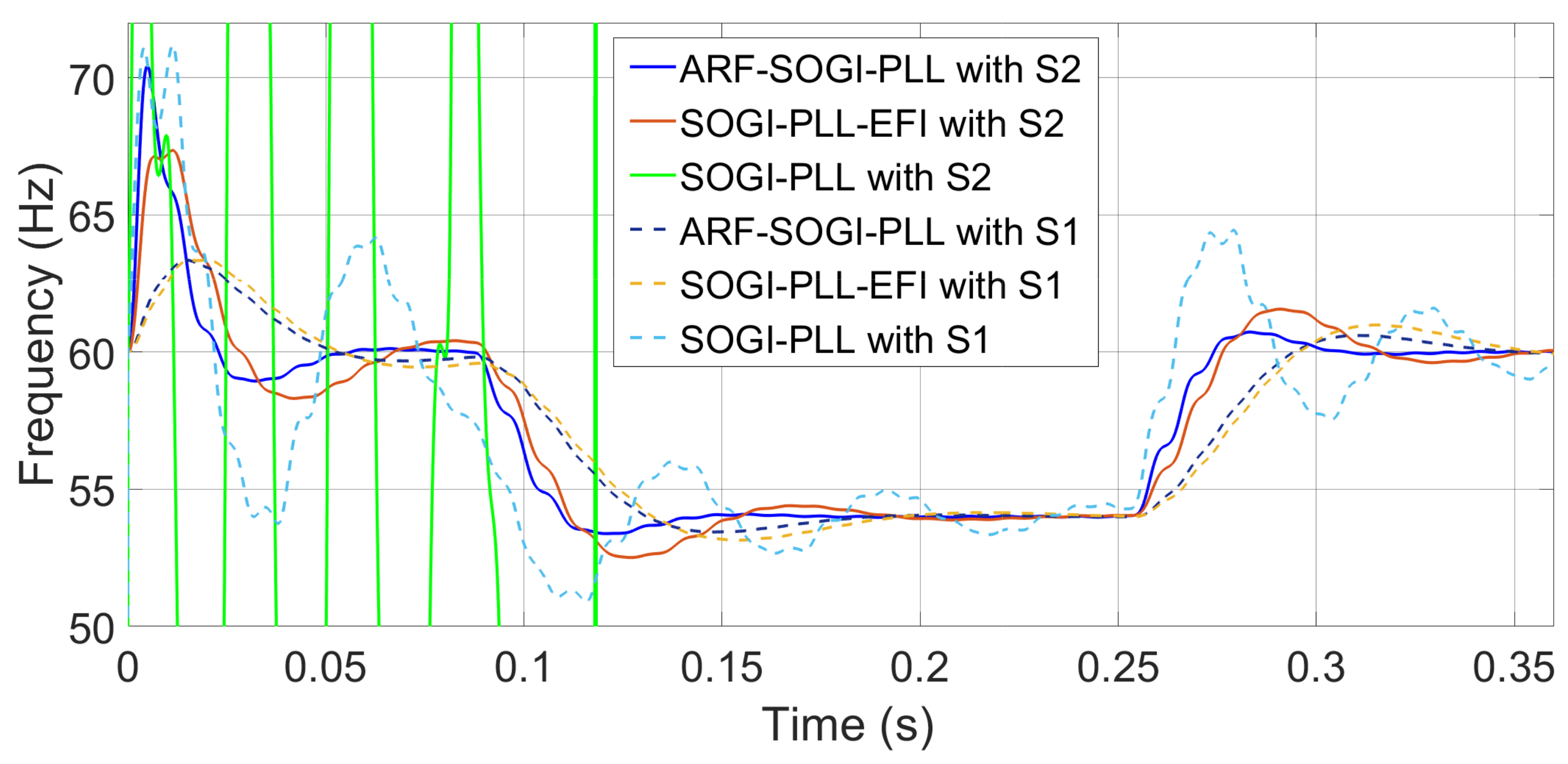
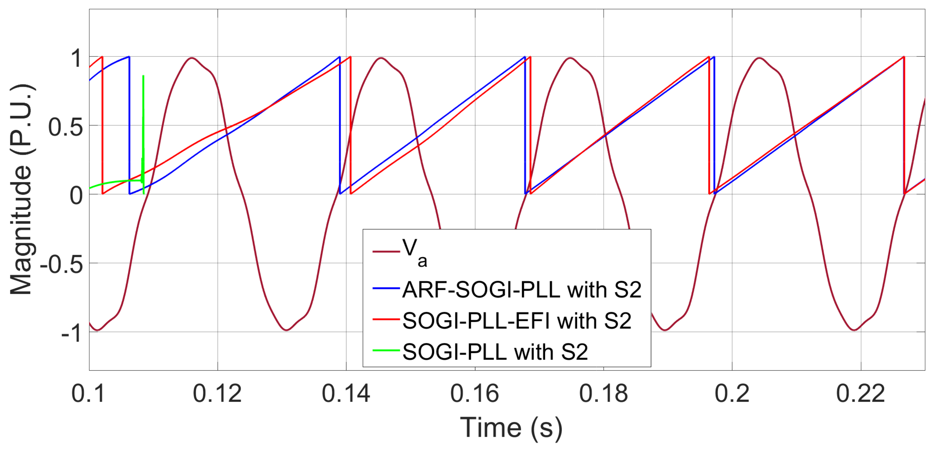
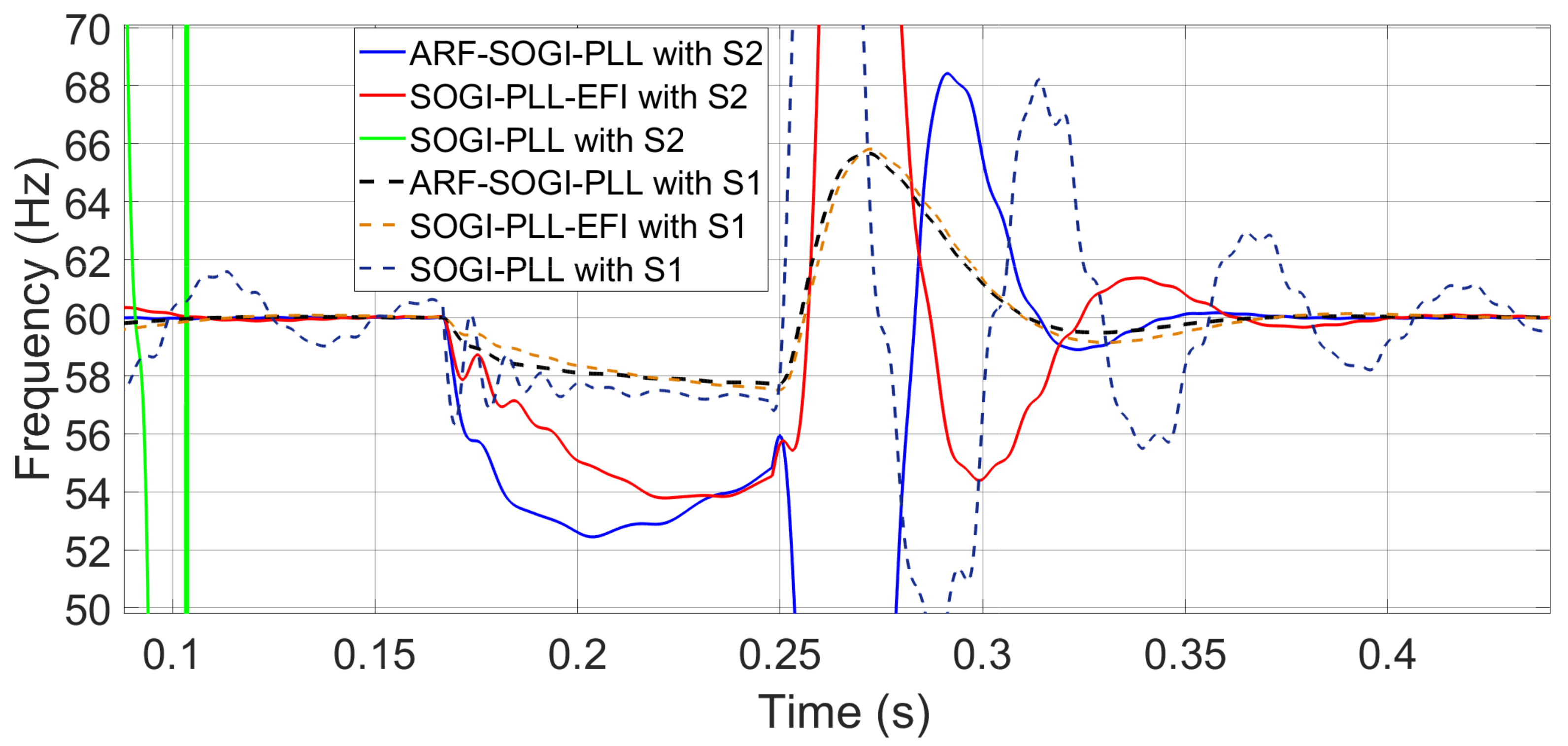
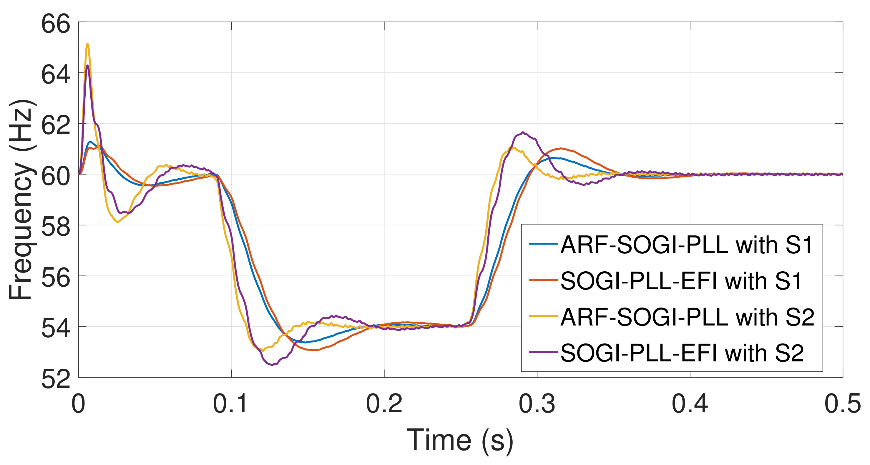
• Frequency deviations of −6 Hz and −14 Hz;
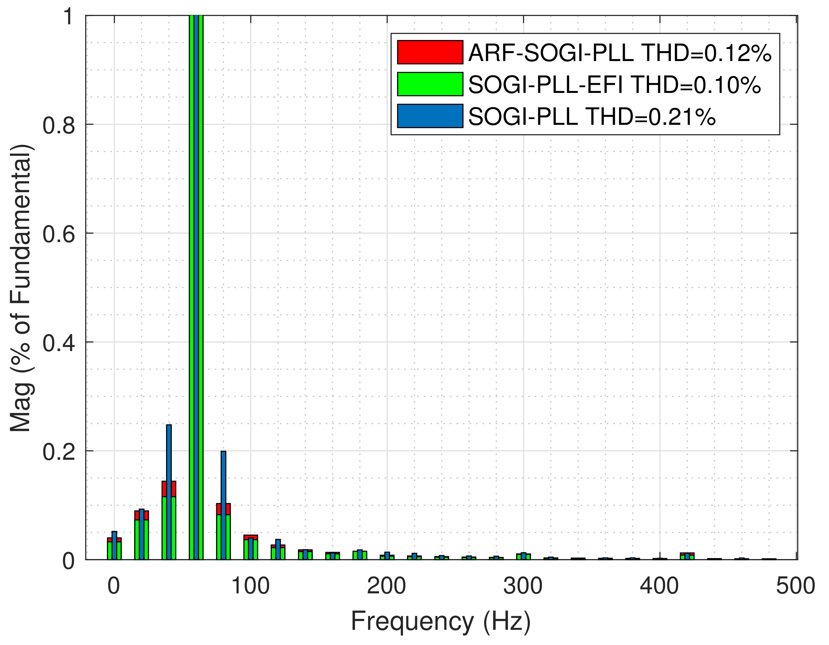
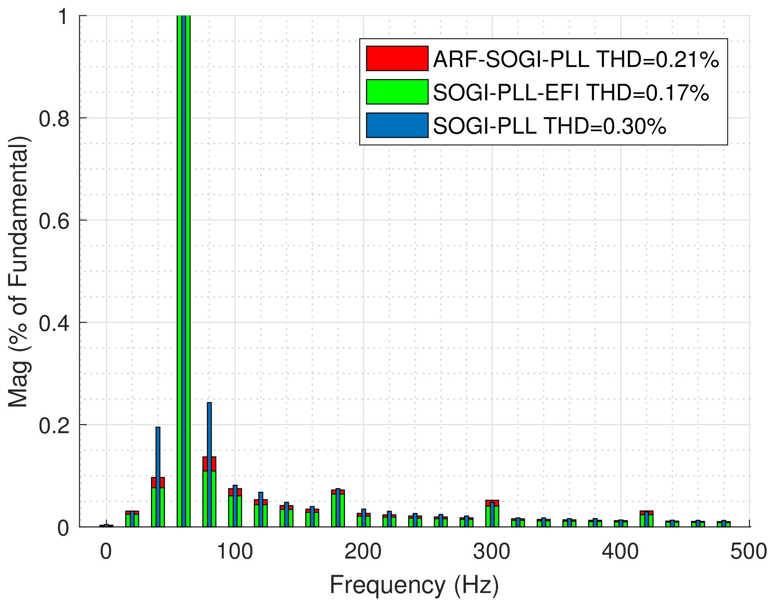
• Harmonic content: 0.04 pu of the fifth harmonic and 0.0295 pu of the seventh harmonic, for a THD = $4.99\%$;
• Phase jump of ${75}^o$;
• Voltage sag of $80\%$;
• Phase-to-ground short-circuit;
• Gain $k=0.5$, to reduce the bandwidth of the SOGIs and better deal with the harmonic content.

The simulations are carried-out using a processor-in-the-loop approach based on the F28335 DSC, so that the real implementation and discretization issues are adequately taken into account. In the co-simulations of this and the following sections, different sets of gains are used to highlight the fact that the performance of the ARF-QSG-PLL is inherent to its architecture regardless of the assigned bandwidths. Three sets of tuning parameters have been used, as detailed in

Table 1. Gains for tuning set S1 (small SOGI bandwidth, typical PLL bandwidth).

	ARF-SOGI			PLL
$k_{\alpha \beta }$	$k_s$	$k_{pre}$	$k_p$	$k_i$
0.5	0.5	1.4	184.7	8479.16
	SOGI			PLL
	k		$k_p$	$k_i$
	0.5		184.7	8479.16

,

Table 2. Gains for tuning set S2 (small SOGI bandwidth, large PLL bandwidth).

	ARF-SOGI			PLL
$k_{\alpha \beta }$	$k_s$	$k_{pre}$	$k_p$	$k_i$
0.5	0.5	1.4	563.67	50,116.247
	SOGI			PLL
	k		$k_p$	$k_i$
	0.5		563.67	50,116.247

and

Table 3. Gains for tuning set S3 (typical SOGI bandwidth, typical PLL bandwidth).

	ARF-SOGI			PLL
$k_{\alpha \beta }$	$k_s$	$k_{pre}$	$k_p$	$k_i$
1.4142	0.5	1.4	184.7	8479.16
	SOGI			PLL
	k		$k_p$	$k_i$
	1.4142		184.7	8479.16

, corresponding to different bandwidths for the QSG and the loop filter.

3. Results

In this section, several verification tests are carried out in order to verify the performance of the proposed ARF-SOGI-PLL. The tests are made with co-simulations implemented under the processor-in-the-loop (PIL) [33,34] approach in MATLAB/Simulink with Code Composer Studio (CCS) and the digital signal controller TMS320F28335 from Texas Instruments.

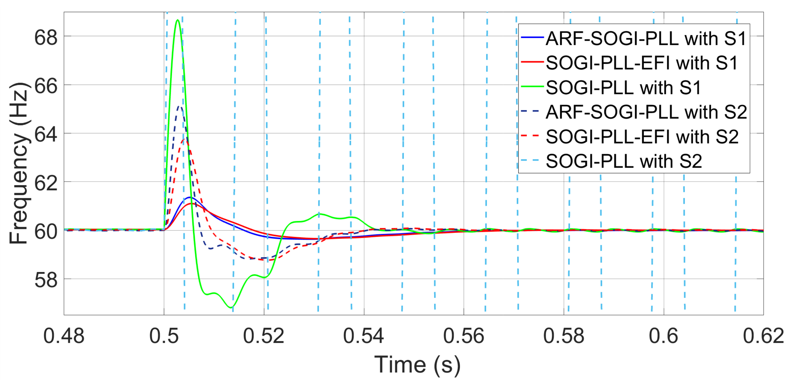
3.1. Response to Frequency Deviation

For this test, the SOGI and ARF-SOGI gains are tuning sets S1 and S2, as specified in Table 1 and Table 2. The response of the schemes to a frequency deviation is shown in Figure 12. It can be seen that the ARF-SOGI-PLL reduces the overshoot in the frequency to lower levels than those reported by both the SOGI-PLL and the SOGI-PLL-EFI. In addition, it also achieves the correct measurement and the steady state in synchronization. For the large bandwidth tuning, this occurs 2.8 cycles before the SOGI-PLL-EFI, as shown in Figure 13.

Another feature of the ARF-SOGI-PLL is that it is possible to almost match its overshoot level, for a large bandwidth loop filter setting, to that of a much smaller typical bandwidth reported by another PLL, such as that of Simulink [26] or any of the versions of SOGI-PLL considered here. In other words, faster PLL response times can be achieved without incurring a high overshoot.

With the tuning set S1, the SOGI-PLL still performs measurement and synchronization, but with high overshoots, and it very slowly reaches the steady state. The SOGI-PLL with the tuning set S2 is no longer able to perform frequency measurement and timing. On the other hand, Figure 13 shows that the ARF-SOGI-PLL synchronizes adequately before the SOGI-PLL. In addition, in the measured frequency, the SOGI-PLL can not synchronize and the signal is lost. This frequency deviation is within the allowed adjustment ranges given in [31,32]. The ARF-SOGI-PLL shows the best behavior, since it synchronizes three cycles before the SOGI-PLL. The ARF-SOGI-PLL is faster when reporting a frequency measurement, and it is more reliable, since its overshoot does not exceed $\pm 1$ Hz. This gives greater assurance that the system will not trip due to an erroneous frequency measurement, compared to the other two versions of the SOGI-PLL considered here.

3.2. Response to Voltage Sag

Voltage sags are a tough test for synchronization algorithms [14,15]; they arise from disturbances in the electrical network, caused by, for example, the energization of transformers or large induction motors [12]. To compare the performance of the PLLs subjected to voltage sag, a test is applied where the grid voltage suddenly changes to 0.2 per unit. The gains of the ARF-SOGI-PLL and the other two PLLs are those of Table 1 and Table 2 (tuning sets S1 and S2). The voltage sag causes a desynchronization of the PLLs; when the fault is cleared, the algorithms must resynchronize. As seen in Figure 14 for the case of a typical PLL bandwidth given by S1, during the resynchronization, the ARF-SOGI-PLL and the SOGI-PLL-EFI report a smooth transient frequency measurement with similar errors. It is also observed that the SOGI-PLL with the typical bandwidth (S1) incurs a large error in the transient frequency measurement and, therefore, the phase tracking error in the resynchronization process is greater than for the other PLLs. For the case of a large PLL bandwidth given by tuning S2, the frequency measurements by the ARF-SOGI-PLL and the SOGI-PLL-EFI are comparable, while the SOGI-PLL is no longer capable of resynchronizing and, therefore, cannot correctly measure the frequency either.

3.3. Response to Ground Fault

Regarding ground faults, during the event, the synchronization is lost by all the algorithms; when the system recovers from the fault, all of the considered SOGI-PLLs re-synchronize after approximately four cycles, except for the standard SOGI-PLL with S2 tuning, as seen in Figure 15. The SOGI-PLL-EFI synchronizes on the third cycle after system recovery; however, it loses synchronization again, regaining it on the fifth cycle, while on the sixth cycle, its error in phase tracking increases. Figure 16 shows the responses for the SOGI-PLL-EFI and the ARF-SOGI-PLL, both using the S2 tuning, in greater detail. Figure 17 shows how, as the resynchronization evolves, the ARF-SOGI-PLL for both tunings (S1 and S2) reports the smallest phase tracking error, synchronizing correctly before the other PLLs. On the other hand, the SOGI-PLL with the S1 tuning can re-synchronize, but it does so slowly, compared to the other two, and reports the highest phase tracking error. For its part, the same PLL with the S2 tuning no longer achieves synchronization.

Moreover, in Figure 17, in the case of the S2 tuning, the ARF-SOGI-PLL reports the lowest error in the phase tracking. The SOGI-PLL-EFI presents an error of zero at $t=0.29$ s (it is synchronized), but when it reaches the next cycle at approximately $t=0.316$ s, it presents an error of $0.05$ s (it loses the correct synchrony). Then, at $t=0.332$ s, the error is reduced to $0.01268$ pu; later, at $t=0.3715$ s, it is synchronized with an error of only $0.000422$ pu, and at $t=0.3902$ s, the error again grows to $0.00424$ pu.

Figure 18 shows that the ARF-SOGI-PLL is the first to report the correct value of the frequency for both tunings S1 and S2. It is also observed how the standard SOGI-PLL with the S1 tuning can measure the frequency of the system by recovering from the short-circuit; however, it is slower, and during the re-synchronization, its measurement has the largest error. The measurement of frequency by the standard SOGI-PLL with the S2 tuning is not seen because, in this case, the initial synchronization is not achieved.

3.4. Harmonic Content Rejection Capability of Large Bandwidth SOGI Versions

The total rejection of the DC component in the orthogonal signal and the improved high-frequency harmonic filtering capability are key features of the SOGI-QSG [35]. For this reason, it is desirable to verify that the proposed ARF-SOGI-PLL does not lose these features. In this section, it is verified that, when using a small-bandwidth (Case A) or a typical-bandwidth (Case B) ARF-SOGI-PLL, the harmonic content rejection capacity is not lost. The loop filters of the PLLs have a common adjustment. The THD of the unit vectors is compared for an input THD of 4.99%.

Case A. The three PLLs considered are adjusted with the gains given in Table 1. Harmonic analysis reveals that the THD of the unit vectors of the PLLs meet the requirement of being less than $1\%$ [36]. However, the THD for the ARF-SOGI-PLL is less than the corresponding value for the SOGI-PLL, and a is little greater than the value for the SOGI-PLL-EFI, as shown in Figure 19.

Case B. The values assigned to the gains of the PLLs are shown in Table 3. For the ARF-SOGI-PLL, THD${}_{\alpha }$=0.12% and THD${}_{\beta }$=0.21%, which is lower than the corresponding values for the SOGI-PLL (THD${}_{\alpha }$=0.21%, THD${}_{\beta }$=0.30%) and slightly higher than the values for SOGI-PLL-EFI (THD${}_{\alpha }$=0.10%, THD${}_{\beta }$=0.17%). In Figure 19 and Figure 20, the harmonic components and THD of the unit vectors $\alpha$ and $\beta$ are compared.

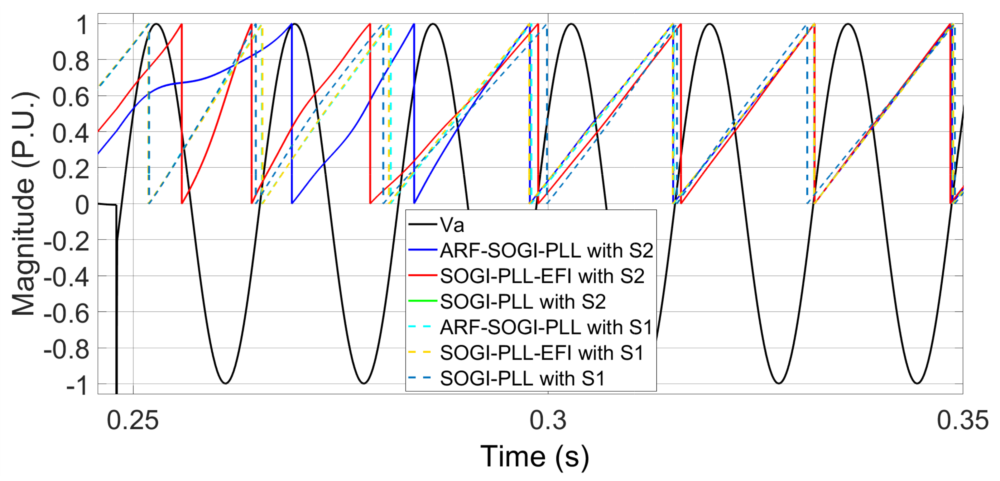
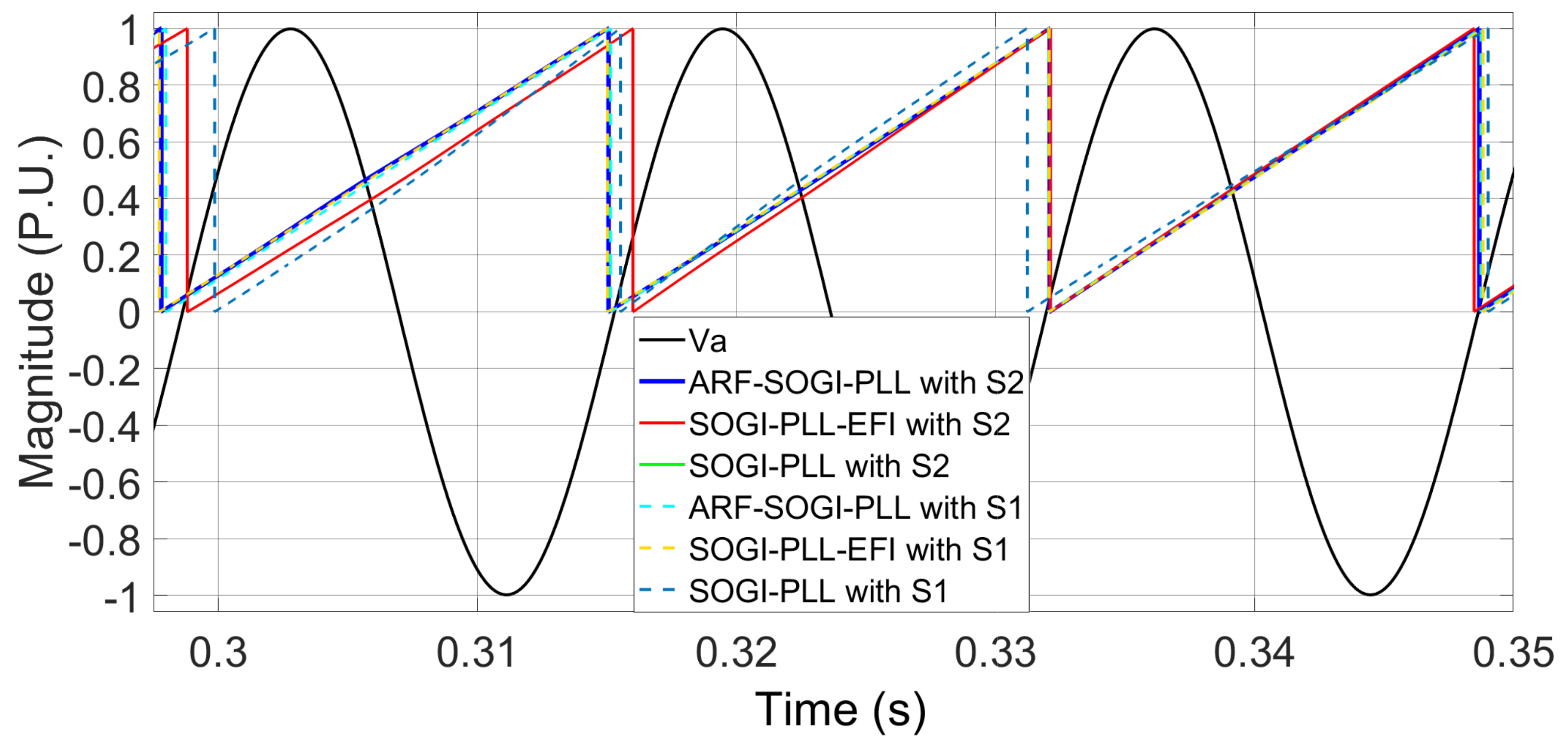
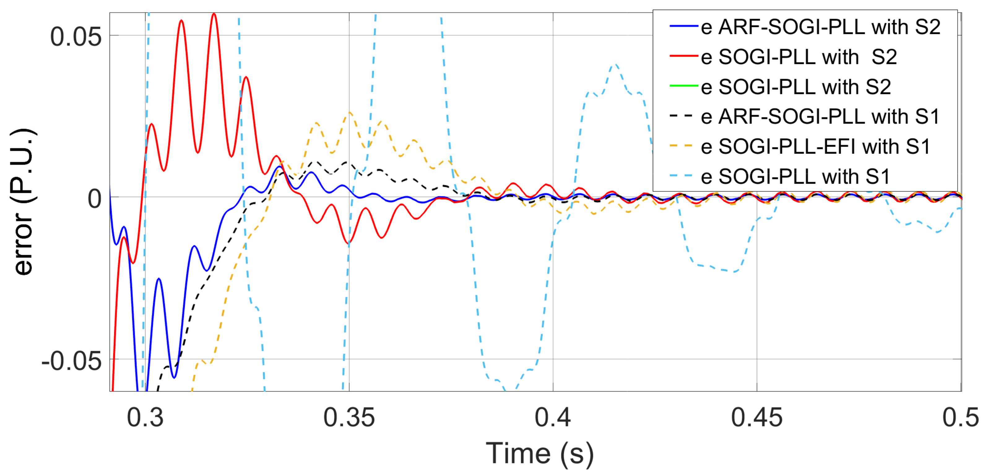
3.5. Synchronization of a Single-Phase Inverter

In this section, the ARF-SOGI-PLL and SOGI-PLL-EFI are used to synchronize a single-phase full-bridge inverter connected to the grid. A comparative analysis of the influence of each PLL on the response of the synchronized inverter is made. Only these two PLLs are considered since they are the ones that have shown the best performance. Figure 21 shows the frequency measurement by the two algorithms using two different settings S1 and S2 during a deviation of $-6\mathrm{Hz}$. The gain values for settings S1 and S2 are listed in Table 1 and Table 2. Figure 21 shows how the ARF-SOGI-PLL achieves a correct frequency before the SOGI-PLL-EFI. The figure also shows that the overshoots given by the ARF-SOGI-PLL at the beginning of the frequency deviations are smaller than those reported by the other PLL. In fact, the overshoot produced by the ARF-SOGI-PLL with a larger bandwidth in its PI is practically the same as that given by the SOGI-PLL-EFI with the smaller bandwidth. This indicates that it is possible to synchronize faster with the ARF-SOGI-PLL than with the SOGI-PLL-EFI.

Figure 22 shows that the ARF-SOGI-PLL syncs 16.67 ms faster than the SOGI-PLL-EFI, and it can be seen that the error in the phase tracking is lower with the ARF-SOGI-PLL.

3.6. Resources and Computing Times

The metrics shown in

Table 4. Required memory and processing time of each algorithm in the DSC.

Algorithm	Flash Memory	Average Execution Time	Maximum Execution Time
SOGI-PLL	4030 bytes (1%)	12,861 ns	14,887 ns
SOGI-PLL-EFI	4013 bytes (1%)	15,136 ns	17,187 ns
ARF-SOGI-PLL in state space	4090 bytes (1%)	13,392 ns	15,307 ns
ARF-SOGI-PLL	4049 bytes (1%)	15,451 ns	17,787 ns

are obtained using a processor-in-the-loop approach. The corresponding measurements are the time necessary for the processing of each of the algorithms in a cycle of the fundamental, and the memory demanded from the 262 KB available in the DSC F28335 processor. Further, in Table 4, it is observed that the flash memory needed by the SOGI-PLL and the SOGI-PLL-EFI is similar, and that it is slightly higher for the ARF-SOGI-PLL.

The memory required by the transfer fuction ARF-SOGI-PLL is greater than the memory required by the SOGI-PLL and SOGI-PLL-EFI versions, but less than the state space ARF-SOGI-PLL. This is seen in Table 4, and it is concluded that the increase in memory required by either of the two implementations of the ARF-SOGI-PLL, with respect to the existing versions of SOGI-PLL, is not a determining factor in a real implementation.

In Table 4, it is seen that the SOGI-PLL is processed faster than any of the others. After this comes the ARF-SOGI-PLL, and the slowest is the SOGI-PLL-EFI. During a run cycle, the ARF-SOGI-PLL resolves 1.744 $\mathsf{\mu }$s faster than the SOGI-PLL-EFI, and 0.531 $\mathsf{\mu }$s slower than the traditional SOGI-PLL. As can be seen in the same Table 4, the modifications made to the SOGI imply raising the processing time of the algorithm.

The ARF-SOGI-PLL implemented in the state space runs 2.059 $\mathsf{\mu }$s faster per DSC processing cycle than the structure of Figure 3. This indicates that, although the memory required by the ARF-SOGI-PLL implemented in the state space is larger than that required by its equivalent in Figure 3, its processing time is lower.

4. Conclusions

The traditional SOGI-PLL is the base for the proposed ARF-SOGI-PLL. The SOGI-QSG transfer functions were brought into the state space representation in controllable canonical form with the intention of having direct access to the sections of the SOGI-QSG algorithm, where gain has an influence. The ARF-SOGI-QSG was proposed, which, unlike the standard SOGI-QSG, contains a second gain $k_s$ that is located in the system matrix in the state space; moreover, a feedback of the output signal of the band-pass filter is added to the input of the modified QSG. These modifications allow for selecting the extra attenuation of the quadrature signals, while moving the QSG poles further to the left, thereby achieving greater stability in the ARF-SOGI-QSG compared to the standard SOGI-QSG.

The block diagram of the ARF-SOGI-QSG and its transfer functions were reported. A linear analysis of the ARF-SOGI-QSG was performed and compared with that of the standard SOGI-QSG, and it was shown that the ARF-SOGI-QSG is a quadrature signal generator with greater stability and a faster response time than that given by the SOGI-QSG.

The greater stability reported by the ARF-SOGI-QSG permits the increase of the bandwidth of the control loop filter, and with that, the response speed of the ARF-SOGI-PLL is increased without compromising the rejection of the harmonic content and without reaching the instability or impossibility of processing compared to the SOGI-PLL.

The complete scheme of a PLL based on the ARF-SOGI-QSG was reported; this proposal was called ARF-SOGI-PLL. To verify the performance of the proposed PLL, this was subjected to different disturbances, such as frequency deviations, phase jumps, voltage sags, phase-to-ground short-circuits, and harmonic contents. The response was compared with the response of two other versions of SOGI-PLL under two different tunings in the loop filter. Finally, a single-phase inverter was synchronized with the voltage of an electrical network. From the simulations, it is confirmed that a PLL based on the new ARF-SOGI-QSG is more stable and faster in its transient response without losing the ability to reject harmonic content.

The responses of the ARF-SOGI-PLL and the SOGI-PLL-EFI are quite similar; however, the ARF-SOGI-PLL can be adjusted in such a way that the overshoot in the frequency measurement is less than the overshoot reported by the SOGI-PLL-EFI. Even when the ARF-SOGI-PLL has a high bandwidth in its loop filter, the overshoot in its response is very similar in magnitude to the overshoot given by the SOGI-PLL-EFI with a lower bandwidth. This contributes to lowering the error in the transient frequency measurements, achieving a correct frequency measurement faster.

The ARF-SOGI-QSG implemented in the state space demonstrated a more agile computational processing. The rejection of the harmonic content in the ARF-SOGI-PLL is better than the rejection given by the traditional SOGI-PLL and it is slightly lower than that presented by the SOGI-PLL-EFI. Although the ARF-SOGI-PLL consumes 77 bytes more than the SOGI-PLL-EFI, the DSC processing of the ARF-SOGI-PLL is 1744 $\mathsf{\mu }$s faster. The ARF-SOGI-PLL requires 60 bytes more than the traditional SOGI-PLL and requires only 0.531 $\mathsf{\mu }$s more in processing time than the traditional SOGI-PLL.

References

1. Best, R.E. Phase-Locked Loops: Design, Simulation, and Applications, 5th ed.; McGraw-Hill: New York, NY, USA, 2003. [Google Scholar]
2. Timbus, A.; Liserre, M.; Teodorescu, R.; Blaabjerg, F. Synchronization methods for three phase distributed power generation systems—An overview and evaluation. In Proceedings of the 2005 IEEE 36th Power Electronics Specialists Conference, Recife, Brazil, 16 June 2005; pp. 2474–2481. [Google Scholar]
3. Best, R.E. Phase-Locked Loops: Design, Simulation, and Applications, 6th ed.; McGraw-Hill Education: New York, NY, USA, 2007. [Google Scholar]
4. Yazdani, A.; Iravani, R. Voltage-Sourced Converters in Power Systems: Modeling, Control, and Applications; John Wiley & Sons: Hoboken, NJ, USA, 2010. [Google Scholar]
5. Golestan, S.; Guerrero, J.M.; Vasquez, J.C. Three-Phase PLLs: A Review of Recent Advances. IEEE Trans. Power Electron. 2017, 32, 1894–1907. [Google Scholar] [CrossRef] [Green Version]
6. Rodríguez, P.; Teodorescu, R.; Candela, I.; Timbus, A.V.; Liserre, M.; Blaabjerg, F. New positive-sequence voltage detector for grid synchronization of power converters under faulty grid conditions. In Proceedings of the 2006 37th IEEE Power Electronics Specialists Conference, Jeju, Korea, 18–22 June 2006; pp. 1–7. [Google Scholar] [CrossRef]
7. Chung, S.K. Phase-locked loop for grid-connected three-phase power conversion systems. IEE Proc.-Electr. Power Appl. 2000, 147, 213–219. [Google Scholar] [CrossRef]
8. Gao, S.; Barnes, M. Phase-locked loop for AC systems: Analyses and comparisons. In Proceedings of the 6th IET International Conference on Power Electronics, Machines and Drives (PEMD 2012), Bristol, UK, 27–29 March 2012; pp. 1–6. [Google Scholar] [CrossRef] [Green Version]
9. Mahdian, H.; Hashemi, M.; Ghadimi, A.A. Improvement in the synchronization process of the voltage-sourced converters connected to the Grid by PLL in order to Detect and Block the Double Frequency Disturbance Term. Indian J. Sci. Technol. 2013, 6, 4940–4952. [Google Scholar] [CrossRef]
10. Jauch, C.; Matevosyan, J.; Ackermann, T.; Bolik, S. International comparison of requirements for connection of wind turbines to power systems. Wind Energy 2005, 8, 295–306. [Google Scholar] [CrossRef]
11. Rodriguez, P.; Luna, A.; Ciobotaru, M.; Teodorescu, R.; Blaabjerg, F. Advanced Grid Synchronization System for Power Converters under Unbalanced and Distorted Operating Conditions. In Proceedings of the IECON 2006—32nd Annual Conference on IEEE Industrial Electronics, Paris, France, 7–10 November 2006; pp. 5173–5178. [Google Scholar] [CrossRef]
12. Teodorescu, R.; Liserre, M.; Rodriguez, P. Grid Converters for Photovoltaic and Wind Power Systems; John Wiley & Sons: New Delhi, India, 2011. [Google Scholar]
13. Karimi Ghartemani, M.; Khajehoddin, S.A.; Jain, P.K.; Bakhshai, A. Problems of Startup and Phase Jumps in PLL Systems. IEEE Trans. Power Electron. 2012, 27, 1830–1838. [Google Scholar] [CrossRef]
14. Abdali Nejad, S.; Matas, J.; Martín, H.; de la Hoz, J.; Al-Turki, Y.A. New SOGI-FLL Grid Frequency Monitoring with a Finite State Machine Approach for Better Response in the Face of Voltage Sag and Swell Faults. Electronics 2020, 9, 612. [Google Scholar] [CrossRef] [Green Version]
15. Abdali Nejad, S.; Matas, J.; Elmariachet, J.; Martín, H.; de la Hoz, J. SOGI-FLL Grid Frequency Monitoring with an Error-Based Algorithm for a Better Response in Face of Voltage Sag and Swell Faults. Electronics 2021, 10, 1414. [Google Scholar] [CrossRef]
16. Bollen, M.H. Understanding power quality problems. In Voltage Sags and Interruptions; IEEE Press: Piscataway, NJ, USA, 2000. [Google Scholar]
17. Rodríguez, P.; Luna, A.; Muñoz-Aguilar, R.S.; Etxeberria-Otadui, I.; Teodorescu, R.; Blaabjerg, F. A Stationary Reference Frame Grid Synchronization System for Three-Phase Grid-Connected Power Converters Under Adverse Grid Conditions. IEEE Trans. Power Electron. 2012, 27, 99–112. [Google Scholar] [CrossRef]
18. Velasco, J.A.M. Power System Transients: Parameter Determination; CRC Press: London, UK, 2010. [Google Scholar]
19. Green, T.; Marks, J. Control techniques for active power filters. IEE Proc.-Electr. Power Appl. 2005, 152, 369–381. [Google Scholar] [CrossRef] [Green Version]
20. Subramanian, C.; Kanagaraj, R. Rapid Tracking of Grid Variables Using Prefiltered Synchronous Reference Frame PLL. IEEE Trans. Instrum. Meas. 2015, 64, 1826–1836. [Google Scholar] [CrossRef]
21. Chung, S.K. A phase tracking system for three phase utility interface inverters. IEEE Trans. Power Electron. 2000, 15, 431–438. [Google Scholar] [CrossRef] [Green Version]
22. Arricibita, D.; Marroyo, L.; Barrios, E.L. Simple and robust PLL algorithm for accurate phase tracking under grid disturbances. In Proceedings of the 2017 IEEE 18th Workshop on Control and Modeling for Power Electronics (COMPEL), Stanford, CA, USA, 9–12 July 2017; pp. 1–6. [Google Scholar] [CrossRef]
23. Nos, O.V.; Abramushkina, E.E.; Kharitonov, S.A. Control Design of Fast Response PLL for FACTS Applications. In Proceedings of the 2019 International Ural Conference on Electrical Power Engineering (UralCon), Chelyabinsk, Russia, 1–3 October 2019; pp. 301–305. [Google Scholar] [CrossRef]
24. Luhtala, R.; Alenius, H.; Roinila, T. Practical Implementation of Adaptive SRF-PLL for Three-Phase Inverters Based on Sensitivity Function and Real-Time Grid-Impedance Measurements. Energies 2020, 13, 1173. [Google Scholar] [CrossRef] [Green Version]
25. Golestan, S.; Ramezani, M.; Guerrero, J.M. An Analysis of the PLLs With Secondary Control Path. IEEE Trans. Ind. Electron. 2014, 61, 4824–4828. [Google Scholar] [CrossRef] [Green Version]
26. Cao, Y.; Yu, J.; Xu, Y.; Li, Y.; Yu, J. An Efficient Phase-Locked Loop for Distorted Three-Phase Systems. Energies 2017, 10, 280. [Google Scholar] [CrossRef] [Green Version]
27. Aldbaiat, B.; Nour, M.; Radwan, E.; Awada, E. Grid-Connected PV System with Reactive Power Management and an Optimized SRF-PLL Using Genetic Algorithm. Energies 2022, 15, 2177. [Google Scholar] [CrossRef]
28. Ciobotaru, M.; Teodorescu, R.; Blaabjerg, F. A new single-phase PLL structure based on second order generalized integrator. In Proceedings of the 2006 37th IEEE Power Electronics Specialists Conference, Jeju, Korea, 18–22 June 2006; pp. 1–6. [Google Scholar] [CrossRef]
29. Ciobotaru, M.; Agelidis, V.G.; Teodorescu, R.; Blaabjerg, F. Accurate and Less-Disturbing Active Antiislanding Method Based on PLL for Grid-Connected Converters. IEEE Trans. Power Electron. 2010, 25, 1576–1584. [Google Scholar] [CrossRef]
30. Guerrero-Rodríguez, N.; Rey-Boué, A.B.; Bueno, E.; Ortiz, O.; Reyes-Archundia, E. Synchronization algorithms for grid-connected renewable systems: Overview, tests and comparative analysis. Renew. Sustain. Energy Rev. 2017, 75, 629–643. [Google Scholar] [CrossRef]
31. IEEE Std 1547a-2020 (Amendment to IEEE Std 1547-2018); IEEE Standard for Interconnection and Interoperability of Distributed Energy Resources with Associated Electric Power Systems Interfaces—Amendment 1: To Provide More Flexibility for Adoption of Abnormal Operating Performance Category III. IEEE: Piscataway, NJ, USA, 2020; pp. 1–16. [CrossRef]
32. IEC61727; Photovoltaic (PV) Systems-Characteristics of the Utility Interface. International Electrotechnical Commission: Geneva, Switzerland, 2004.
33. Motahhir, S.; Ghzizal, A.E.; Sebti, S.; Derouich, A. MIL and SIL and PIL tests for MPPT algorithm. Cogent Eng. 2017, 4, 1378475. [Google Scholar] [CrossRef]
34. Krishna Srinivasan, M.; Daya John Lionel, F.; Subramaniam, U.; Blaabjerg, F.; Madurai Elavarasan, R.; Shafiullah, G.M.; Khan, I.; Padmanaban, S. Real-Time Processor-in-Loop Investigation of a Modified Non-Linear State Observer Using Sliding Modes for Speed Sensorless Induction Motor Drive in Electric Vehicles. Energies 2020, 13, 4212. [Google Scholar] [CrossRef]
35. Golestan, S.; Guerrero, J.M.; Vasquez, J.C. Single-Phase PLLs: A Review of Recent Advances. IEEE Trans. Power Electron. 2017, 32, 9013–9030. [Google Scholar] [CrossRef]
36. Kulkarni, A.; John, V. Analysis of Bandwidth–Unit-Vector-Distortion Tradeoff in PLL During Abnormal Grid Conditions. IEEE Trans. Ind. Electron. 2013, 60, 5820–5829. [Google Scholar] [CrossRef]
Figure 1. Structure of the traditional SOGI-PLL.
Energies 15 04253 g001
Figure 2. State space architecture of the ARF-SOGI-QSG.
Energies 15 04253 g002
Figure 3. Block diagram representation of the ARF-SOGI-QSG.
Energies 15 04253 g003
Figure 4. Bode diagrams of the SOGI-QSG versions for v .
Energies 15 04253 g004
Figure 5. Bode diagrams of the SOGI-QSG versions for q v .
Energies 15 04253 g005
Figure 6. SOGI-QSG and ARF-SOGI-QSG band-pass filter v poles.
Energies 15 04253 g006
Figure 7. SOGI-QSG and ARF-SOGI-QSG low-pass filter q v poles.
Energies 15 04253 g007
Figure 8. v ARF-SOGI-QSG poles.
Energies 15 04253 g008
Figure 9. q v ARF-SOGI-QSG poles.
Energies 15 04253 g009
Figure 10. q v low-pass filter-step response of the SOGI-QSG versions.
Energies 15 04253 g010
Figure 11. Structure of the ARF-SOGI-PLL.
Energies 15 04253 g011
Figure 12. Frequency measured using a high bandwidth and a typical bandwidth in the PLLs in the face deviation of −6 Hz in the frequency of the line voltage.
Energies 15 04253 g012
Figure 13. ω t measured during −6 Hz deviation to before 60 Hz recovery.
Energies 15 04253 g013
Figure 14. Frequency before, during and after a voltage sag of 80 % .
Energies 15 04253 g014
Figure 15. ω t during and after phase-to-ground short-circuit fault using a high and typical bandwidth in the control loop of the PLLs.
Energies 15 04253 g015
Figure 16. ω t during the synchronization process, from the third to the sixth cycle after system recovery following a phase-to-ground short-circuit.
Energies 15 04253 g016
Figure 17. Phase tracking error from third to sixth cycle after system recovery from phase-to-ground short-circuit.
Energies 15 04253 g017
Figure 18. Frequency measured before, during, and after phase-to-ground short-circuit fault.
Energies 15 04253 g018
Figure 19. THD of the unit vectors α = cos ω t for k α β = 0.5 and k = 0.5 and an input THD of 4.99 % .
Energies 15 04253 g019
Figure 20. THD of the unit vectors β = sin ω t for k α β = 0.5 and k = 0.5 and an input THD of 4.99 % .
Energies 15 04253 g020
Figure 21. Frequency measured following −6 Hz deviation during 0.166 s, and its recovery, using a high bandwidth and a typical bandwidth in the PLLs control loop.
Energies 15 04253 g021
Figure 22. ω t in the final cycle in the synchronization of the ARF-SOGI-PLL.
Energies 15 04253 g022