An Efficient Framework to Estimate the State of Charge Profiles of Hydro Units for Large-Scale Zonal and Nodal Pricing Models

Abstract

The power system is undergoing significant changes so as to accommodate an increasing amount of renewably generated electricity. In order to facilitate these changes, a shift from the currently employed zonal pricing to nodal pricing is a topic that is receiving increasing interest. To explore alternative pricing mechanisms for the European electricity market, one needs to solve large-scale nodal optimization problems. These are computationally intensive to solve, and a parallelization or sequencing of the models can become necessary. The seasonality of hydro inflows and the issue of myopic foresight that does not display the value in storing water today and utilizing it in the future is a known problem in power system modeling. This work proposes a heuristic step-wise methodology to obtain state of charge profiles for hydro storage units for large-scale nodal and zonal models. Profiles obtained from solving an aggregated model serve as guidance for a nodal model with high spatial and temporal resolution that is solved in sequences. The sequenced problem is guided through soft constraints that are enforced with different sets of penalty factors. The proposed methodology allows for adjustments to congestions on short timescales and proves to perform well in comparison to other approaches to this issue suggested in the literature. Following the input profile closely on a long timescale renders good results for the nodal model.

1. Introduction

This section provides, firstly, a motivation for the presented study. On a higher level, the significance of this work is embedded in a policy context. Regarding the applicability of the method to perform electricity market design and nodal pricing studies, the ongoing debate on nodal and zonal pricing in a European context is briefly laid out. Lastly, the technical motivation for the proposed methodology is given. A thorough literature review on, firstly, existing nodal pricing models and, secondly, on addressing hydro storage issues in models is presented. Lastly, this section sums up the main contributions of this work.

1.1. Motivation

The energy system is undergoing significant changes in the face of the decarbonization and the integration of increasing renewable energy sources into the electricity mix. Furthermore, the European Commission is aiming to increasingly integrate the European electricity market, and advancing the Energy Union [1]. While it has become internationally accepted that a transition of the electricity system is direly needed, these efforts have been accelerated in the face of recent events. Due to the conflict in Ukraine, an energy crisis has erupted. The international community is increasing its efforts to become independent of Russian imports of fossil fuels and, most importantly, natural gas. The European Commission has recently launched the REPowerEU strategy, which sets out a roadmap to speed up the transition to clean energy sources and to become less dependent on Russia [2]. Thus, also the transformation of the electricity system will see an increased speed. These challenges call for investigation of the future design of the electricity market. Currently, the European market relies on zonal pricing, where cross-zonal transmission capacities give rise to different prices in zones, while intra-zonal transmission capacities are not reflected in market prices. An alternative that is receiving increasing interest is nodal pricing, where the whole transmission network is considered and reflected in the price formation [3]. In order to investigate this market design for the whole of Europe, one needs to solve large optimal power flow (OPF) problems, ideally, over longer time horizons [4]. This is a task that is computationally challenging, and it is common to subdivide an OPF problem into smaller ones through, e.g., parallelization or sequencing. In this context, the modeling of hydro storages becomes an issue that needs to be carefully addressed. There are different dimensions to the representation of hydro storages in a large-scale model. The inflow to hydro storages has an underlying seasonality, which, together with long-term variations of demand, need to be reflected in a long-term model. Displaying seasonality in a long-term model that is subdivided into smaller problems is not a straightforward task. Further, when minimizing costs for a sub-problem of a larger problem, foresight is not provided. That is, the optimization would behave in a greedy fashion and utilize hydro storage capacities early on in the optimization horizon due to myopic foresight. Lastly, accurate representation of hydro storage reservoirs requires the consideration of intertemporal constraints to maintain the continuity of reservoir levels, which calls for a sequentialization, rather than a parallelization, of the large problem. Furthermore, when aiming to assess nodal against zonal markets, it is necessary to ensure comparability between two models representing these two market design options. Due to the different spatial resolution of nodal and zonal models, this poses questions regarding various aspects. In the context of hydro modeling, comparability can be achieved by utilizing the same underlying hydro profiles for both models. Given the fact that accurate data on pan-European hydro reservoir levels are scarce, these so-called state of charge (SOC) profiles need to be determined from simulations. Therefore, it is necessary to follow a sound methodology to obtain SOC profiles to ensure that the issues of seasonality and myopic foresight are addressed. Additionally, such method poses an opportunity to provide the comparability between zonal and nodal models of the European electricity system. Thus, the primary motivation for this work presents the challenge of sound hydro storage modeling in long-term energy system models.

1.2. Literature Review

The European electricity market is currently based on zonal pricing, where a uniform electricity price is determined for every bidding zone. Bidding zones follow predominantly country borders. This approach to price formation disregards physical limitations to electricity flow. The lack of displaying intra-zonal capacity limits in the price-making gives rise to congestions and instabilities in the network and calls for remedial actions such as congestion management [5,6]. The concept of nodal pricing is gaining increasing interest as a possible remedy to these and other issues in electricity prices and network representation [7]. Physical capacity limits of the grid are respected when determining nodal prices; this can thus reduce the need for redispatching and send correct price signals to the market [8].

The European Commission [9], in its impact assessment, has investigated four possibilities for improving local price signals to improve dispatch decisions and investments in the EU wholesale market [3]. It is stated that a switch from zonal to nodal pricing would incorporate the value of available transmission capacity across market regions, which would utilize available resources more efficiently. The impact assessment further points out that for electricity markets and networks, nodal pricing is theoretically the most optimal pricing system and would render remedial actions by TSO to alleviate congestion unnecessary. However, implementing nodal pricing in the European internal electricity market would imply a fundamental change to the structure of markets, the management of the grid, and trading mechanisms and was, for the time being, deemed disproportionate. Further, stakeholders expressed concerns about creating a single EU Independent System Operator; instead, a step-wise regional integration of system operation is preferred. Thus, currently, there are some regulatory barriers to implementing nodal pricing in the European electricity system, as well as some opposition by stakeholders, that would need to be overcome. Thus, sound modeling of the electricity system is needed to provide further indications to assess the costs and benefits.

Various studies have focused on modeling electricity markets based on nodal pricing in comparison to zonal pricing. In [10] a three-level unit commitment model is introduced, where the day-ahead market, the intra-day market, and the real-time balancing market are solved simultaneously for every hour of the day. The potential benefits of creating an integrated European electricity market are analyzed in [11] through an agent-based model, where cross-border congestion management and capacity mechanisms are examined explicitly. These are investigated with respect to their impact on two system performance measures, i.e., market-wide welfare and adequacy. In a case study on Central Western Europe, they confirm the benefits entailed by cross-border market coupling and the furthering of market harmonization across Europe. Reference [12] developed a two-step zonal model that, first, minimizes generation cost subject to amongst other the zonal grid configuration, and secondly, congestion management is modeled through a cost minimization that regards the network’s capacity limits in greater detail. In their nodal model, these two steps are combined into one. They investigate the distributional impacts of a switch from zonal to nodal pricing in Germany. Through the allocation of financial transmission rights (FTR), the implications of price changes on individual actors can be mitigated. In their case study, they find that the distributional effects on the demand side and also largely on the conventional generation can be successfully mitigated with the right allocational design of FTR. However, they identified more challenges with regard to intermittent renewable generation, where a more sophisticated FTR design is needed to facilitate an effective switch from zonal to nodal pricing. A hybrid zonal–nodal pricing model is investigated in [13]. A welfare maximization emulated the day-ahead market, where capacity limits are respected in the nodal pricing areas. Consecutively, the cost minimal redispatching is determined that avoids exceeding capacity limits of lines. The hybrid zonal–nodal pricing model is applied to a case study including the Czech Republic, Germany, Poland, and Slovakia. In their scenario, Poland adopts a nodal pricing scheme and they investigate a case of business as usual and one of high wind penetration. They find that Poland can benefit from a shift to a nodal pricing scheme, as it helps them manage impacts on their grid caused by their vicinity to wind power generation units. Poland is able to reduce their needs for redispatching. At the same time, [13] find that a country such as Germany with a diverse supply and demand structure can benefit from keeping a zonal pricing scheme, as it helps them maintain a relatively low electricity price level throughout the entire country. The need to combine market and grid models in order to perform studies that can assess the increased integration of renewable energy sources (RESs) into the electricity system is stressed in [14]. When exploring future scenarios for the power system, the market perspective can only be a starting point, as especially grid extension and operational issues will play a vital role in the future evolution of the system. Thus, they propose a soft-linked combined market and grid model. They apply their model to a case study on the German system and study the level of congestion due to a zonal dispatch of generators. They conclude that, especially given the spatial distribution of RES, a detailed representation of the grid and all power systems components is vital for a sound contingency analysis of future power systems. Given the various modeling design options and possible applications, it is evident that there is no single best model yet developed suitable to model nodal pricing, especially in comparison to zonal pricing.

It is suggested in [15] that nodal pricing would also result in more efficient management of hydro resources, especially in countries with predominantly hydro generation technologies. Hydro storages already play a major role in the generation of electricity, especially in countries such as Norway, where they make up around 88% of the installed generation capacity [16]. The marginal costs to produce hydroelectric power are very low, and further, there are no carbon emissions entailed with the generation of power. This alone could render hydro an important energy resource of the future. Additionally, hydro plants are a flexible source of electricity as water is stored in reservoirs, and pumped hydro storage units can even store electricity [17]. However, hydro also poses some unique challenges to the design and operation of power markets. A study on hydro-dominated markets in China identified as major challenges the uncertainties of runoff and prices, bidding among different stakeholders of cascaded hydropower plants, the modeling, and clearing of such markets, the coordination of trading with multiple timescales, and the relevance of trans-provincial and trans-regional transmission capacities [18].

The significance of sound hydro storage modeling in medium-term electricity market models, as well as different approaches to do so, have been studied in various research. An overview of the different hydropower modeling challenges is given in [19]. One of the significant difficulties is linked to the time horizon simulated. For short-term models with a high time resolution, operational constraints are the main modeling issue, while the accurate long-term optimization of hydro storage reservoirs is not the central task. Medium-term hydro optimization is concerned with the seasonality of reservoirs and inflows as well as the storage aspects throughout a year. Long-term models are more oriented toward investigating climatic fluctuations and the impacts on the hydrological system. They discuss the application of soft constraints to model hydro storages and the difficulties of choosing penalty costs correctly and balancing well between different objectives. Lastly, run-time requirements are identified as a major challenge and discussed in the context of finding a trade-off between accuracy and computational tractability. They also discuss the use of cost functions to forecast the future value of water stored in hydro reservoirs. This is especially relevant when optimizing a model in sequence over a longer time horizon. This needs to be carried out through additional constraints to account for the time-dependent factors. In an empirical study assessing the performance of electricity markets with hydroelectric reservoir storages, the key features of markets with hydroelectricity were identified to be the intertemporal aspects that water can be stored to be utilized at a later point in time, which calls to include opportunity and shortage costs in the calculation of marginal costs of hydropower plants [20]. The relevance of hydro storages for zonal modeling and the impact it has on different pricing regimes is explored by [21]. They investigate the challenges that hydro storage dispatch also poses in the context of congestion management and different zonal configurations. In EUDispatch, a zonal model of the European electricity system, the seasonality of hydro is captured through a preliminary run where a temporal aggregation of the model allows obtaining weekly SOC profiles. These serve as input to simulations with hourly resolutions that are performed in sequences of a week. The weekly SOC profiles provide fixed target values for the beginning and end of each simulation step [22,23]. The hydro unit commitment problem formulated as a mixed-integer linear program to minimize costs and in particular focus on mitigating data errors and infeasibility issues is studied in [24]. They suggest providing fixed operational points to hydro facilities, as well as mid-horizon and final target volumes. Through the introduction of marginal corrective slacks into their model, they eliminate infeasibility issues through a two-stage method. They test their methodology on real-world test cases that are comparatively small. The standardized bidding procedure for the dispatch of hydro storages in Norway is discussed in [25]. They describe the use of water values to be utilized as bidding prices in long- and medium-term models. In [26], several modeling approaches to consider hydroelectric plants in energy models are reviewed. They report that the water value is more appropriate to display a hydro facility operator’s marginal revenue instead of the traditional system marginal cost [27]. While under some circumstances constant bid prices for hydro power can be used [28], it is rather common to work with dynamic bid prices. These bids are deduced as shadow prices of the hydro storage reservoir continuity constraint [29,30,31].

1.3. Contribution and Structure of the Paper

In the literature, there exist methods to deal with the issue of myopic foresight of hydro storages in zonal models of the European electricity system; however, when there is a high spatial resolution, this issue is not addressed well. These methods rely on a spatial and temporal resolution that is not necessarily applicable to problems that inspect a large number of nodes and accordingly of generation and storage units. The method of water values is used, where either shadow prices from a model that is solvable are passed, or constant prices are assigned to hydro storages. The former entails the problem that an aggregated model will not include all the information, especially with regard to the transmission network, and thus it will also not be displayed in SOC profiles, while the latter lacks fluctuations in water value throughout the year, missing the aspect of seasonality.

To address these shortcomings, we propose a novel heuristic algorithm. Our step-wise method uses the hydro storage profiles from a spatially aggregated model and passes it to the full-resolution problem, which is then guided by the profiles while not tightly bound to them. Thereby, new SOC profiles are obtained that reflect the long-term evolution of the power system, including also the line capacities, which are considered in greater detail in the higher-resolution model. Thanks to the developed heuristic, we obtain SOC profiles that allow us to solve large-scale nodal and zonal optimization problems in sequence and perform comparative studies between the two pricing mechanisms.

The remainder of the paper is structured in the following fashion. Section 2 introduces the problem at hand in more detail and provides the mathematical formulation of it. In Section 3, the methodology to obtain hydro state of charge profiles for a large economic dispatch model is described. We describe the numerical experiments and their results in Section 4 and formulate conclusions in Section 5.

2. Problem Statement

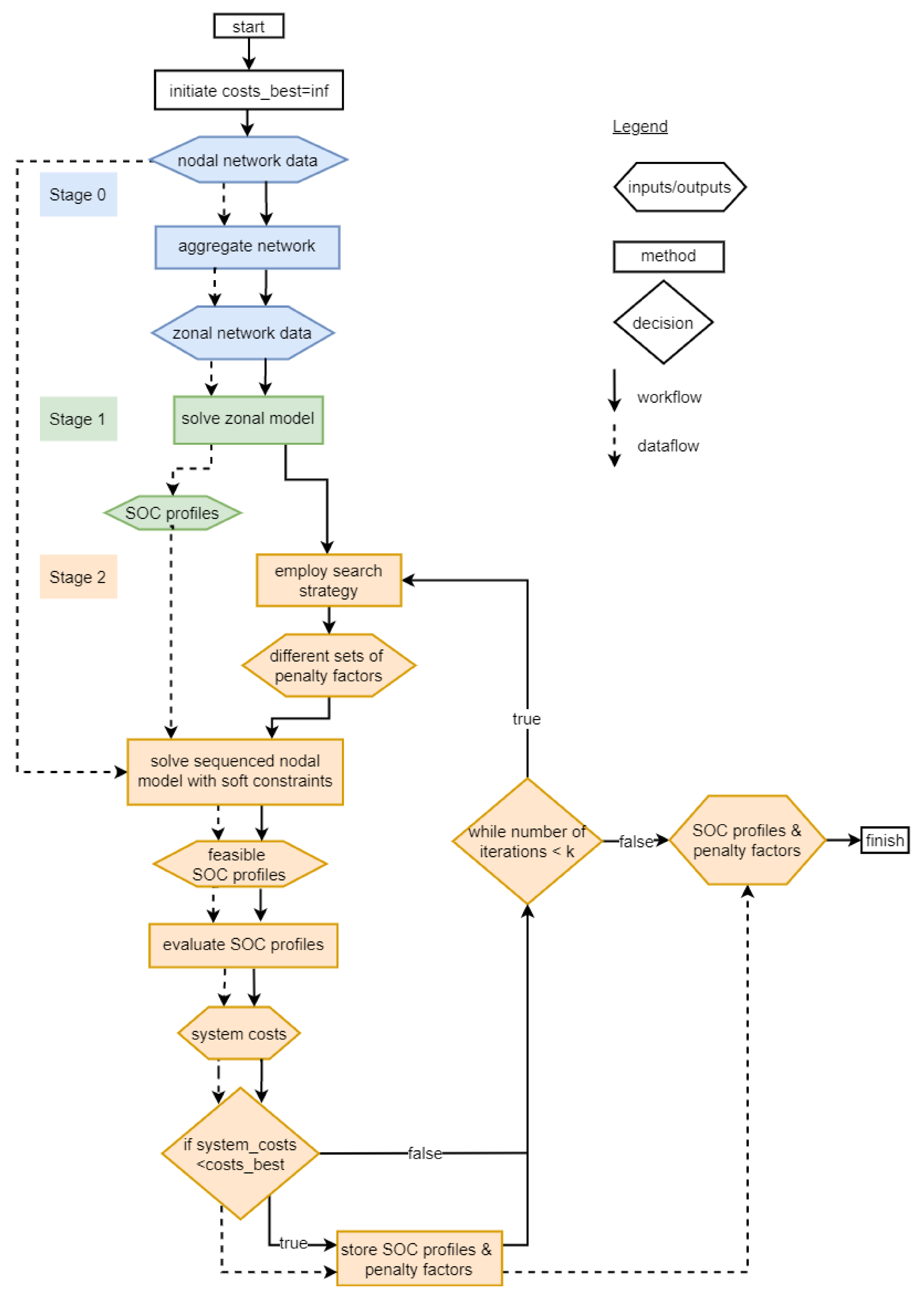
In this section, the different aspects defining the problem will be laid out. We want to investigate the European electricity market under a nodal pricing regime. Nodal pricing based on so-called locational marginal prices (LMP) is opposed to the currently existing zonal pricing mechanism in Europe. In each zone z in Europe, where $z\in Z$ is the set of all zones, there will be uniform prices, while under nodal pricing, LMPs will be determined at every node n, which can be down to the resolution of individual substations, and the set of all nodes is N. Prices will differ when transmission line capacity limits are exceeded, and the flow $F_{nm}$ from node n to node m reaches the capacity limit ${\overline{F}}_{nm}$ or the sum of cross-zonal flows from zone z to zone $y\in Z\left(z\right)$, which border on zone z. Cross-zonal flows are found as the sum of flows in transmission lines $F_{nm}$ from nodes n in the set of nodes $\widehat{N}\left(z\right)$ belonging to zone z to node m that are in the set of nodes connected to node n and are also in $\widehat{N}\left(y\right)$, the set of nodes connected to zone y. For comparative studies, the compatibility between the two approaches is essential; this reflects in particular on network representation. In order to calculate LMPs, one has to solve a large optimization problem. We formulate the problem as an economic dispatch model [14,32,33,34,35,36], which in its full formulation reads:

$$\begin{array}{l}\mathrm{minimize}{\displaystyle \sum _{t\in T}}\left({\displaystyle \sum _{g\in \mathcal{G}}}{P}_{g,t}·c_g+{\displaystyle \sum _{s\in S}}{P}_{s,t}^{dis}·c_s\right)\end{array}$$

(1)

$$\begin{array}{l}\mathrm{subject}\mathrm{to}\\ \sum _{d\in D\left(n\right)}{P}_{d,t}=\sum _{m\in N\left(n\right)}{F}_{mn,t}+\sum _{g\in \mathcal{G}\left(n\right)}{P}_{g,t}+\sum _{s\in S\left(n\right)}\left(P_{s,t}^{dis}-P_{s,t}^{stor}\right),\forall n\in N,t\in T\end{array}$$

(2)

$$\begin{array}{cc}\hfill F_{nm,t}& =B_{nm}({\mathsf{\Theta }}_{n,t}-{\mathsf{\Theta }}_{m,t}),\forall n\in N,m\in N^{\prime }\left(n\right),t\in T\hfill \end{array}$$

(3)

$$\begin{array}{cc}\hfill F_{nm,t}& =-F_{mn,t},\forall n\in N,m\in N\left(n\right),t\in T\hfill \end{array}$$

(4)

$$\begin{array}{cc}\hfill \beta ·{\overline{F}}_{nm}& \le F_{nm,t}\le \beta ·{\overline{F}}_{nm},\forall n\in N,m\in N\left(n\right),t\in T\hfill \end{array}$$

(5)

$$\begin{array}{cc}\hfill {NTC}_{yz}& \le \sum _{n\in \widehat{N}\left(z\right)}\sum _{m\in N\left(n\right)\cap \widehat{N}\left(y\right)}{F}_{nm,t}\le {NTC}_{zy},\forall z\in Z,y\in Z\left(z\right),t\in T\hfill \end{array}$$

(6)

$$\begin{array}{cc}\hfill 0& \le P_{g,t}\le {\overline{P}}_g,\forall g\in {\mathcal{G}}_{conv},t\in T\hfill \end{array}$$

(7)

$$\begin{array}{cc}\hfill 0& \le P_{g,t}\le {\overline{P}}_g·p_{g,t}^{avail},\forall g\in {\mathcal{G}}_{res},t\in T\hfill \end{array}$$

(8)

$$\begin{array}{cc}\hfill 0& \le P_{s,t}^{dis}\le {\overline{P}}_s,\forall s\in S,t\in T\hfill \end{array}$$

(9)

$$\begin{array}{cc}\hfill 0& \le P_{s,t}^{stor}\le {\overline{P}}_s,\forall s\in S,t\in T\hfill \end{array}$$

(10)

$$\begin{array}{cc}\hfill 0.3·{\overline{SOC}}_s& \le so{c}_{s,t}\le {\overline{SOC}}_s,\forall s\in S,t\in T\hfill \end{array}$$

(11)

$$\begin{array}{cc}\hfill so{c}_{s,t}& =so{c}_{s,t-1}+{\eta }^{stor}·P_{s,t-1}^{stor}-\frac{1}{{\eta }^{dis}}·P_{s,t-1}^{dis}+inf{l}_{s,t-1}-spil{l}_{s,t-1},\forall s\in S,t\in T.\hfill \end{array}$$

(12)

The objective Function (1) is minimized over all time steps t in the time horizon $T=\{t_1,t_2,\cdots ,t_{end}\}$. The objective includes the costs to generate power from all generation units $\mathcal{G}$ and storage units S. Individual units’ costs are calculated from $c_g$, the marginal costs of generator g, and the dispatched power $P_{g,t}$ of generator g at time t, and $c_s$ the marginal costs of storage unit s and the dispatched power $P_{s,t}^{dis}$ of storage unit s at time t. The nodal power balance is defined in Equation (2), which ensures that at every time t the sum of demand $P_{d,t}$ of all the loads $d\in D\left(n\right)$ connected to node n equals the sum of flows $F_{mn}$ entering from adjacent nodes $N\left(n\right)$, the generation $P_{g,t}$ from all generators $\mathcal{G}\left(n\right)$ connected to node n, and the net power dispatch of storage units $S\left(n\right)$ connected to node n, which is the difference between dispatched power $P_{s,t}^{dis}$ and stored power $P_{s,t}^{stor}$. Equation (3) describes the relation between power flow $F_{nm,t}$ in AC lines and voltage angles ${\mathsf{\Theta }}_n$, where $B_{nm}$ is the susceptance of the line connecting node n and adjacent nodes $m\in N^{\prime }\left(n\right)$ connected via an AC line. In the network, there are also high-voltage DC (HVDC) lines, in which the power flow is not determined by the physical properties of the lines but is considered controllable. Therefore, for power flows $F_{nm,t}$ in HVDC lines, only the conservation of flow is enforced in Equation (4). This relation applies to both flows through AC and through HVDC lines from node n to adjacent node $m\in N\left(n\right)$. Power flow in transmission lines is limited in Equation (5) by the thermal capacity of lines ${\overline{F}}_{nm}$, which are reduced through the factor $\beta$. Including a fixed reliability margin is a practice that is also proposed in the literature to approximate security constraints [33]. Equation (6) limits the cross-zonal flow from zones $z\in Z$ to adjacent zones $y\in Z\left(z\right)$ to the net-transfer capacities $NT{C}_{zy}$. Power generation from conventional units ${\mathcal{G}}_{conv}$, renewable units ${\mathcal{G}}_{res}$, and storages, as well as power consumption for storage, is limited by upper capacity constraints ${\overline{P}}_g$ and ${\overline{P}}_s$, respectively, in Equations (7)–(10). The power generation constraints (8) from renewable energy sources solar and wind are further limited by a time-dependent reduction factor $p_{g,t}^{avail}$ of maximum power ${\overline{P}}_g$ output of renewable generator g at time t due to weather fluctuation. The filling of hydro storage expressed through the state of charge $so{c}_{su,t}$ is limited by upper and lower limits (Equation (11)); the lower limit is set at 30% of the total capacity ${\overline{SOC}}_s$. In Equation (12), the intertemporal continuity constraint for hydro storages is defined. It ensures that $so{c}_{su,t}$, the state of charge of unit s at time t, equals the state of charge at $t-1$ plus the storage power $P_{s,t-1}^{stor}$ at $t-1$ with the storage efficiency ${\eta }^{stor}$, minus the dispatched power $P_{s,t-1}^{dis}$ at $t-1$, where ${\eta }^{dis}$ is the dispatch efficiency, plus $inf{l}_{s,t-1}$ the inflow to storage unit s at time $t-1$ and minus $spil{l}_{s,t-1}$, the spillage of storage unit s at $t-1$. The optimization variables are $P_{g,t}$, $P_{s,t}^{dis}$, $P_{s,t}^{stor}$, $so{c}_{s,t}$, and ${\mathsf{\Theta }}_{n,t}$. LMPs will be derived as dual variables of constraints (2).

Given the size of the European transmission grid, solving this optimization problem is computationally highly intensive. It can be computationally tractable for short time periods, but in the case of performing simulations for an entire year with an hourly resolution, computation times can become very large, and simulations can only be conducted on high-performance computers. In a previous study, we investigated the computational times for different formulations of the optimal power flow problem and found that while the DC approximation will be solvable in polynomial time, a large number of nodes and a long-time horizon still lead to very high computational times [37]. Therefore, it becomes necessary to perform so-called rolling horizon simulations, where the model is solved in sequences. Computations in parallel are not possible because of intertemporal constraints. These concern, in the linear program formulation of the economic dispatch problem, only hydro storage units and, in particular, the SOC of reservoirs (Equation (12)). Given the seasonality of inflows to hydro reservoirs and the fact that hydro units function not only as generation but also as storage units, the seasonality needs to be accounted for. However, in a rolling horizon simulation, the model has myopic foresight, and the optimization will be greedy and utilize the energy stored in hydro reservoirs within the first sequences. This is because information about future opportunities to dispatch hydropower in times of peak prices is not available to the optimization.

Therefore, it is necessary to develop a heuristic that passes the information about the seasonality of inflows as well as the benefits of storing energy today and utilizing it in the future. As mentioned above, the comparability of nodal outcomes to a zonal model is interesting when assessing the potential benefits of nodal pricing. While a nodal model clearly has to rely on a much higher spatial resolution than a zonal model, the two are linked through constraints (6). The question of comparability can be extended to the described issue of hydro storage modeling, and the utilization of zonal hydro profiles as inputs to the nodal model poses a possibility to take this into account.

3. Methodology

In this section, the proposed methodology to obtain SOC profiles for the large nodal model described in Section 2 is introduced.

As the computational efforts to run the full models with an hourly resolution are large, simulations need to be performed in sequence. Therefore, the issue of hydro storage units arises, i.e., the model would utilize all the stored water in the reservoirs and empty them within the first sequences if there was no foresight included. Thus, we propose a heuristic step-wise modeling framework, which is illustrated in Figure 1. Utilizing heuristic approaches in hydropower optimization is an increasingly researched topic [38]. Initially, in Stage 0, data are collected and prepared to serve as inputs for the full nodal and a spatially aggregated zonal model. In Stage 1, the zonal model is run for the entire time horizon to produce initial SOC profiles. These serve as input to Stage 2, in which the nodal model is run in sequences and guided by the input profiles through soft constraints. These soft constraints are implemented through slack variables, which contribute to the objective function of the optimization problem and thus also require the setting of penalty factors that quantify this contribution; therefore, a set of penalty factors is another input to Stage 2. Finally, we evaluate the produced SOC profiles by assessing the overall system costs of generating power and storing the best-performing input parameters. In the following, we describe Stage 1 and Stage 2 in more detail, whereas the data preparation Stage 0 is explained further in Section 4.1.1.

Stage 1. The target is to produce SOC profiles for an entire year from a spatially aggregated model that is referred to as zonal model. As has been mentioned in the literature review, solving aggregated models to obtain hydro profiles is a common approach. The main difference in comparison to the nodal model introduced in Equations (1)–(12) is the level of network representation. Instead of including all network constraints, the zonal model solely regards inter-zonal capacity limits. These capacities are displayed through the net-transfer capacities (NTC) [23,34,36]. Besides the fact that the zonal model can be run in a reasonable amount of time for the whole reference year with an hourly resolution, it also emulates the European electricity day-ahead market, as it is functioning in its current design. The full mathematical description of the problem reads:

$$\begin{array}{cc}\hfill \mathrm{minimize}& {\displaystyle \sum _{t\in T}}\left({\displaystyle \sum _{g\in \mathcal{G}}}{P}_{g,t}·c_g+{\displaystyle \sum _{s\in S}}{P}_{s,t}^{dis}·c_s\right)\hfill \end{array}$$

(13)

$$\begin{array}{l}\mathrm{subject\; to}\\ \sum _{d\in \widehat{D}\left(z\right)}{P}_{d,t}=\sum _{y\in Z\left(z\right)}{F}_{zy,t}+\sum _{g\in \widehat{\mathcal{G}}\left(z\right)}{P}_{g,t}+\sum _{s\in \widehat{S}\left(z\right)}\left(P_{s,t}^{dis}-P_{s,t}^{stor}\right),\forall z\in Z,t\in T\end{array}$$

(14)

$$\begin{array}{cc}\hfill F_{zy,t}& =-F_{yz,t},\forall z\in Z,y\in Z\left(z\right),t\in T\hfill \end{array}$$

(15)

$$\begin{array}{c}\hfill \begin{array}{cc}\hfill {NTC}_{yz}& \le F_{zy,t}\le {NTC}_{zy},\forall z\in Z,y\in Z\left(z\right),t\in T\hfill \end{array}\end{array}$$

(16)

$$\left(7\right)–\left(12\right)$$

Equation (13) is the objective function, where the overall costs of generating power from generators and storage units are minimized. The power balance in Equation (14) ensures that for all times t, all power consumed by demands $\widehat{D}\left(z\right)$ at zone z equals the sum of all power generated from generators $\widehat{\mathcal{G}}\left(z\right)$, the net power output of storage units $\widehat{S}\left(z\right)$, and the sum of flows $F_{zy,t}$ going into zone z from adjacent zones $y\in Z\left(z\right)$. Equation (15) ensures that imports $F_{zy,t}$ to zone z from zone y equal exports $F_{yz,t}$ from zone z to zone y. This represents a generic flow model, where flow conservation at zones is maintained. Flows in cross-zonal lines $F_{zy,t}$ are limited by upper $NT{C}_{zy}$ and lower $NT{C}_{yz}$ capacity limits, the so-called net transfer capacities, expressed in Equation (16). The constraints for power generation and storage units were already introduced in Equations (7)–(12) and are the same as in the nodal model. Resulting from this initial run of the zonal model, we obtain a hydro profile for the hourly SOC of all the storage units present in the system. These profiles are then aggregated to a zonal level, which means that all storage units’ SOCs within a zone are aggregated to obtain hourly SOC profiles for each zone. This profile, along with all the SOC profiles of individual storage units, functions as input to the next step.

Stage 2. The purpose of this stage is twofold; firstly, to produce feasible profiles for the nodal model, and secondly, to adjust the profiles to the more-constraint situation of the nodal network. Given the discrepancy between the zonal and nodal network representation, the outcomes of the former stage are not necessarily feasible in the nodal model. Therefore, we use the SOC profiles for individual storage units and zones from Stage 1 as target values, but we do not enforce that they are being met strictly. Thus, we introduce a set of soft constraints that penalize deviations from the zonal input profiles by adding a penalty term to the objective function. The nodal optimization model will be run in sequences. We only introduce these soft constraints at the end of each sequence; thereby, we allow complete freedom to deviate from the input profile throughout the sequence, which is a technique commonly employed in hydroelectric modeling [39,40]. Thus, the model should be able to react to short-term incentives as line overloadings or peaks in prices, while overall, the trend is followed through the soft constraint at the end of each sequence. The first step in the sequence represents an exception, as there, the constraints are also present at the beginning of the sequence time window. This is because, in the consecutive steps, the initial SOC values will be passed on from the previous step to ensure continuity, while in the first step, there is no input to be passed. Thereby, the problem is considering a trade-off between minimizing overall costs and following the target profiles, which, if not followed, increase the objective function value through penalties. We have a sequence of I smaller optimization problems i, where each is solved for the set of times $T_i=\{t_{i,1},t_{i,2},\cdots ,t_{i,end}\}$. The set of $T_i$ make up the whole time horizon $T=\{T_1,T_2,\cdots ,T_I\}$. The formulation of problems $i\ne 1$ reads:

$$\mathrm{minimize}\sum _{t\in T_i}\left(\sum _{g\in \mathcal{G}}{P}_{g,t}·c_g+\sum _{s\in S}{P}_{s,t}^{dis}·c_s\right)+$$

(17)

$$+\sum _{s\in S}{a}_{s,t=t_{i,end}}·{\alpha }_s+\sum _{z\in Z}{a}_{z,t=t_{i,end}}·{\alpha }_z$$

$$\begin{array}{l}\mathrm{subject}\mathrm{to}\\ a_{s,t}& \ge so{c}_{s,t}-SO{C}_{s,t}^{target},\forall s\in S,t=t_{i,end}\end{array}$$

(18)

$$\begin{array}{cc}\hfill -a_{s,t}& \le so{c}_{s,t}-SO{C}_{s,t}^{target},\forall s\in S,t=t_{i,end}\hfill \end{array}$$

(19)

$$\begin{array}{cc}\hfill a_{z,t}& \ge \sum _{s\in \widehat{S}\left(z\right)}so{c}_{s,t}-SO{C}_{z,t}^{target},\forall z\in Z,t=t_{i,end}\hfill \end{array}$$

(20)

$$\begin{array}{c}\hfill \begin{array}{cc}\hfill -a_{z,t}& \le \sum _{s\in \widehat{S}\left(z\right)}so{c}_{s,t}-SO{C}_{z,t}^{target},\forall z\in Z,t=t_{i,end}\hfill \\ \hfill \left(2\right)& -\left(12\right)\hfill \end{array}\end{array}$$

(21)

$$\begin{array}{cc}\hfill SO{C}_{s,t}^{min}& \le so{c}_{s,t},\forall s\in S,t=t_{i,end}.\hfill \end{array}$$

(22)

The objective function Equation (17) includes, next to the costs of generating power, also the penalty contributions for the SOC target values. These contributions come from the slack variables $a_{s,t}$ for the deviations from the input target values $SO{C}_{s,t}^{target}$ for individual storage units s (Equations (18) and (19)) and the slack variables $a_{z,t}$ for the deviations from the input target values $SO{C}_{z,t}^{target}$ for the sum of storage units $s\in \widehat{S}\left(z\right)$ connected to zone z (Equations (20) and (21)). These deviations from the input profiles are penalized with the respective penalty factors ${\alpha }_s$ for individual storage units and ${\alpha }_z$ for the sum of SOC in a zone, to quantify the contribution to the objective function. Equations (2)–(12) have already been introduced for the full nodal model. Equation (22) ensures that at the end of every sequence a minimum level of $SO{C}_{s,t}^{min}$ is reached for each storage unit s, so that the cyclic constraint (Equation (12)) can also be met for the overall time horizon. To understand how these minimum target values are determined, it is necessary to differentiate between two types of hydro storages, which are pumped hydro storages (PHS) and hydro dams. The target values for each storage unit s at the end of the overall time horizon at $t_{end}$$SO{C}_{s,t=t_{end}}^{min}$ are determined from Equation (12). Starting from this, the target values are backcasted for storage units s belonging to the set of all PHS units $S_{phs}$ following:

$$SO{C}_{s,t=t_{end}-(j+1)}^{min}=SO{C}_{s,t=t_{end}-j}^{min}-{\eta }^{stor}·{\overline{P}}_s^{stor},\mathrm{for}j=0,1,2,\cdots ,t_{end}-1.$$

(23)

The minimum target value of SOC at every hour needs to be at least the target value of the previous hour minus the maximum storage pumping power times the corresponding efficiency, which can fill up the storage reservoir. On the other hand, storages s belonging to the set of all dam hydro storages $S_{dam}$ can be refilled by natural inflows; therefore, their minimum SOC target values are determined from

$$SO{C}_{s,t=t_{end}-(j+1)}^{min}=SO{C}_{s,t=t_{end}-j}^{min}-inf{l}_{s,t=t_{end}-j},\mathrm{for}j=0,1,2,\cdots ,t_{end}-1.$$

(24)

Now, as mentioned above, the formulation of the optimization problem differs only for the first step in the sequence, because there, also soft constraints for the first hour in the sequence are present. The problem for $T_1=\{t_{1,1},t_{1,2},\cdots ,t_{1,end}\}$, the first step in the sequence, reads:

$$\begin{array}{c}\mathrm{minimize}\hspace{1em}\sum _{t\in T_1}\left(\sum _{g\in \mathcal{G}}{P}_{g,t}·c_g+\sum _{s\in S}{P}_{s,t}^{dis}·c_s\right)+\end{array}$$

(25)

$$\begin{array}{l}\begin{array}{}\\ & +\sum _{s\in S}\left(a_{s,t=t_{1,1}}·{\alpha }_s+a_{s,t=t_{1,end}}·{\alpha }_s\right)+\\ \hfill & +\sum _{z\in Z}\left(a_{z,t=t_{1,1}}·{\alpha }_z+a_{z,t=t_{1,end}}·{\alpha }_z\right)\hfill \end{array}\end{array}$$

$$\begin{array}{l}\mathrm{subject}\mathrm{to}\\ a_{s,t}\ge so{c}_{s,t}-SO{C}_{s,t}^{target},\forall s\in S,t=\{t_{1,1},t_{1,end}\}\end{array}$$

(26)

$$\begin{array}{cc}-a_{s,t}& \le so{c}_{s,t}-SO{C}_{s,t}^{target},\forall s\in S,t=\{t_{1,1},t_{1,end}\}\hfill \end{array}$$

(27)

$$\begin{array}{cc}{a}_{z,t}& \ge \sum _{s\in \widehat{S}\left(z\right)}so{c}_{s,t}-SO{C}_{z,t}^{target},\forall z\in Z,t=\{t_{1,1},t_{1,end}\}\hfill \end{array}$$

(28)

$$\begin{array}{l}-a_{z,t}\le \sum _{s\in \widehat{S}\left(z\right)}so{c}_{s,t}-SO{C}_{z,t}^{target},\forall z\in Z,t=\{t_{1,1},t_{1,end}\}\\ \left(2\right)-\left(12\right).\end{array}$$

(29)

Here, Equations (26)–(29) enforce the target values also at the first hour of the first sequence, as opposed to Equations (18)–(21) of the consecutive steps in the sequence, where they are only applicable to the last time step in the sequence. As discussed above, this is because the initial SOC levels are passed as inputs to consecutive steps to the intertemporal storage units constraints (Equation (12)).

After solving the sequence of nodal models with soft constraints, we assess the overall system costs as the costs of generating power, and if the result outperforms the costs obtained with the previously best SOC profile, we store the SOC profiles and the penalty factors that led to them. Then, we employ a search strategy to generate different penalty factor combinations as inputs and perform the sequenced nodal model run again and assess the costs until we reach the number of previously defined iterations. This method is applied to benchmark cases introduced in the next section, which also briefly describes the data preparation (see Stage 0 in Figure 1).

4. Results

In this section, we present the design of experiments along with a description of the inputs and data preparation firstly. Then, we show the results from the conducted numerical experiments for four different scenarios and discuss the performance of the proposed framework to obtain hydro SOC profiles for large-scale zonal and nodal electricity market models.

4.1. Benchmarks

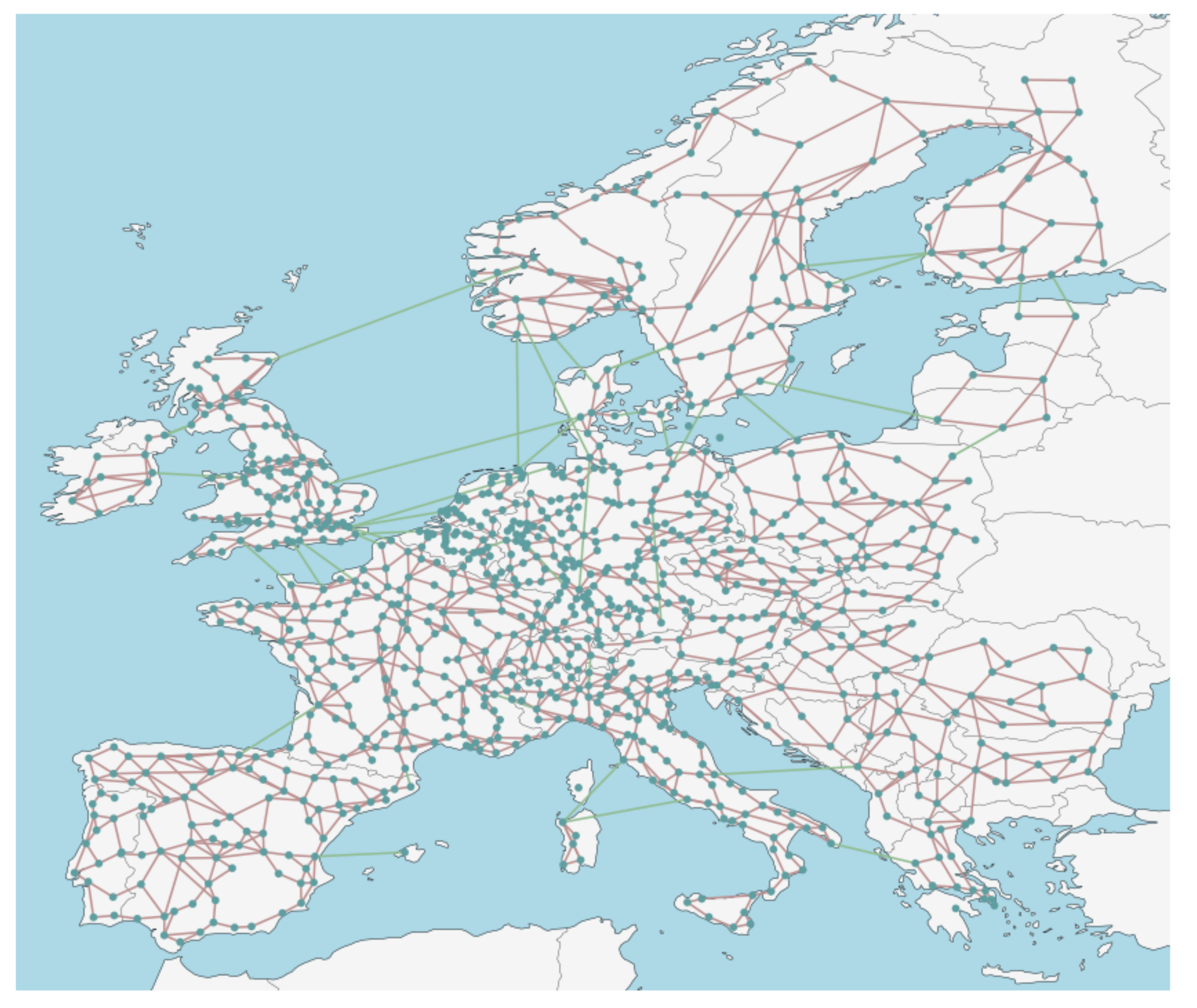
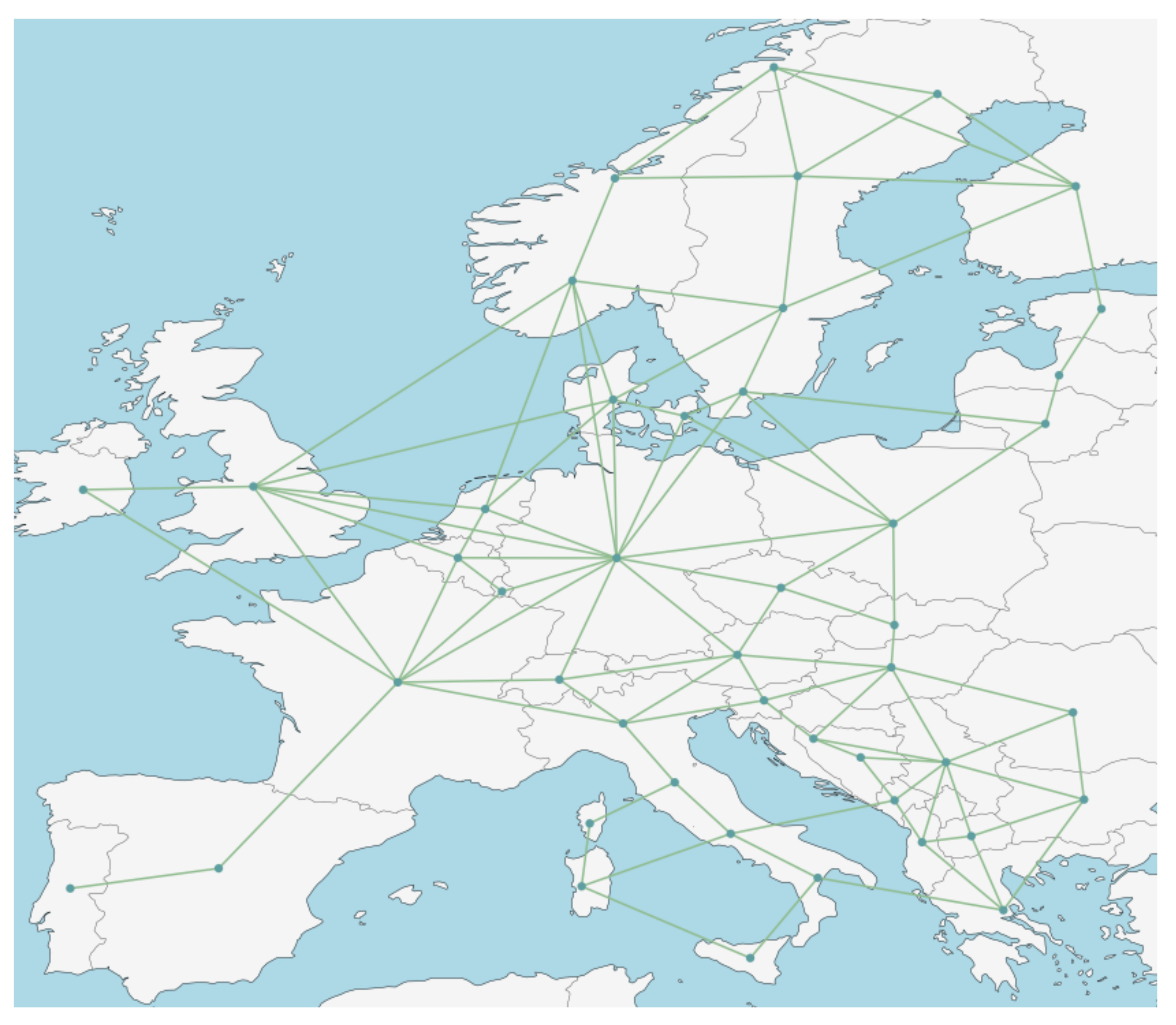
4.1.1. Nodal and Zonal Network Preparation

In this section, the workflow to build up the base dataset is laid out. This corresponds to Stage 0 of the proposed methodology (see Figure 1). The model is implemented in Python using the open-source tool PyPSA [32]. The base network is built using PyPSA-Eur [41]. PyPSA-Eur is an open-source tool that can build and solve networks of the European transmission system from various data sources. The network comprises transmission line capacities and physical properties; connected to nodes are generators and loads; for RESs, capacity availability factors are assigned to nodes that are time series indicating the maximum capacity percentage that can be dispatched for solar and wind plants connected to the respective node. As the base year, we chose 2018 because of data availability. PyPSA-Eur is used to build the base network of 1010 nodes for Europe (included in the model are the following countries: Albania, Austria, Belgium, Bosnia and Herzegovina, Bulgaria, Croatia, Czech Republic, Denmark, Estonia, Finland, France, Germany, Great Britain, Greece, Hungary, Ireland, Italy, Latvia, Lithuania, Luxembourg, Montenegro, Netherlands, North Macedonia, Norway, Poland, Portugal, Romania, Serbia, Slovakia, Slovenia, Spain, Sweden, and Switzerland).

In a consecutive step, the nodal model is aggregated to 45 zones, which approximates the reality of the zonal market in Europe in 2018. In this aggregating step, all transmission lines are removed and replaced with inter-zonal transport lines with their NTCs. The NTCs are taken from ENTSO’s ten-year net development plan (TYNDP) and are assumed constant throughout the year [42]. Flows through these new lines will be modeled through a transport model, i.e., it is a generic flow model, where only flow conservation at a node is maintained. Therefore, only line capacities need to be provided to the model, as opposed to the DC approximation of power flow, where also physical line properties as the susceptance need to be known. All other components (generators, storage units, and loads) are reassigned to zones in accordance with the geographical location of the node they were assigned to in the nodal network. However, the level of detail for all the generation and storage units, as well as loads, is maintained. This is performed in order to maintain comparability between the zonal and the nodal network models. This becomes especially relevant when the ultimate aim of applying these models is to compare them, also including redispatching. The resulting nodal and zonal networks are illustrated in Figure 2 and Figure 3.

4.1.2. Experimental Design

The goal is to determine the utilization of hydro storages through the methodology described above. In particular, the state of charge time series for the different storage units should be determined. The model is implemented in Python and relies heavily on the PyPSA package [32]. The optimization problems are solved using the commercial solver Gurobi. Simulations are conducted on a cluster node with two ten-core Intel Xeon processors and 750 GB RAM. We compare the method described above in Step 2 against other approaches proposed in the literature [25,28,29,30,31]. Concretely, against using hydro shadow prices derived from constraint (12) in Stage 1 of the zonal optimization, we further compare the proposed methodology against using constant bid prices for hydro, which are chosen to be higher than the marginal costs to produce electricity from hydro storages.

We investigate the different methods to obtain hydro SOC profiles under four different scenarios. We analyze two different simulation time horizons, four months and the whole year. Simulating an entire year is common practice in electricity market modeling. The shorter horizon is chosen as computations of the full nodal model are achievable in reasonable computational times. We run simulations with an hourly resolution. For the sequenced nodal model described in Stage 2, we choose sequences of one week. We employ a grid search as a search strategy to generate the penalty factors that are inputs for the sequenced nodal model with soft constraints. Then, we are able to compare the SOC profiles obtained from the different methods to the SOC profile determined from an optimization that simulates the entire four months in one simulation step and is therefore regarded as the optimal profile. We then vary the capacity of transmission lines to simulate situations of higher congestion. In the base scenario, we use 70% of line capacity ($\beta =0.7$), as this value is commonly used to approximate the N-1 criterion [43]. We then reduce the available transmission line capacity to 50% of the thermal capacity.

The quality of profiles is measured through different performance indicators. We analyze the objective function value or overall system costs, the level of congestion, the amount of demand not served (load shedding), and the computational times. As a measure of congestion, we use the system congestion proposed by [44]. The system congestion $s{c}_t$ at time t is measured through the standard deviation of the locational marginal prices (LMP):

$$s{c}_t=\sqrt{\frac{1}{N}\sum _{n\in N}{\left({\overline{LMP}}_t-LM{P}_{n,t}\right)}^2},$$

(30)

where $LM{P}_{n,t}$ is the LMP at node n at time t, and ${\overline{LMP}}_t$ is the average LMP over all nodes N at time t. LMPs are derived as dual variables of Equations (2) and (14) of the zonal and the nodal model, respectively [45]. In the following, we assess the numerical results using the average system costs $\overline{sc}$ over the whole time horizon.

4.2. Results: Benchmarks with Short-Time Horizon

In this section, we present the results for the benchmark case with the short-time horizon of four months. We report on the overall system costs, the level of congestion, and the amount of load shedding, as well as the computation times. The results are presented for the full nodal model run with an hourly resolution (referred to as $NODAL$), which optimizes the entire four months in one simulation ((1)–(12)); the heuristic to obtain SOC profiles described in Section 3, denoted by $SOC\_HEUR({\alpha }_z,{\alpha }_s)$ with the different penalty factor combinations for the two $\alpha$; and the methods described in the literature, we denote the one relying on shadow prices derived from Equation (9) as $SH\_PRICES$ and the one relying on constant bid prices $BIDS\left(bidprice\right)$.

An overview of outcomes for the short-time horizon benchmark with transmission capacity factor $\beta =0.7$ is presented in

Table 1. Results overview for the short-time horizon benchmark with transmission capacity factor $\beta =0.7$. Reported are for the different methods: the total system costs, which are made up of operational costs (i.e., power generation costs) and load shedding costs, the difference between $NODAL$ and the respective method in absolute amount and relative to the total system costs of $NODAL$; the average system congestion ($\overline{sc}$); the total amount of load shed and the share of this amount with respect to the total load; and the run times.

	Costs					Congestion	Load Shedding		Run Time
Method	System [B EUR]	Operational [B EUR]	Load Shedding [B EUR]	Difference System-NODAL [B EUR]	Difference System-NODAL wrt NODAL [%]	$\overline{\mathbf{sc}}$	Amount [GWh]	Share of Tot Demand [%]	Run Time [h]
ZONAL	20.07	20.07	0.00	−0.98	−4.7	7.7	0	0.000	0.6
NODAL	21.05	20.63	0.42	0.00	0.0	663.4	42	0.004	184.8
SH_PRICES	42.13	21.49	20.64	21.08	100.2	858.9	2064	0.208	1.3
BIDS(20)	42.31	21.49	20.83	21.27	101.1	861.5	2083	0.210	1.5
BIDS(40)	40.02	21.48	18.54	18.97	90.1	853.2	1854	0.187	1.2
BIDS(60)	43.34	21.53	21.81	22.30	106.0	861.2	2181	0.220	1.4
SOC_HEUR(1000,1000)	21.06	20.64	0.42	0.01	0.1	663.4	42	0.004	11.6
SOC_HEUR(1000,10)	21.06	20.64	0.42	0.01	0.1	663.4	42	0.004	4.9
SOC_HEUR(1000,0)	21.06	20.65	0.42	0.02	0.1	663.4	42	0.004	36.6
SOC_HEUR(10,1000)	21.06	20.64	0.42	0.01	0.1	663.4	42	0.004	22.5
SOC_HEUR(10,10)	21.44	20.84	0.60	0.39	1.9	675.0	60	0.006	2.0
SOC_HEUR(10,0)	21.52	20.91	0.60	0.47	2.2	675.0	60	0.006	1.6
SOC_HEUR(0,1000)	21.06	20.64	0.42	0.01	0.1	663.4	42	0.004	14.5
SOC_HEUR(0,0)	43.92	21.44	22.49	22.88	108.7	863.3	2249	0.227	1.3

.

The overall system costs obtained for most of the penalty factor combinations are in a similar range, while the best performing combination penalty factors are $SOC\_HEUR(1000,1000)$, $SOC\_HEUR(1000,10)$, $SOC\_HEUR(10,1000)$, and $SOC\_HEUR(0,1000)$, which differ only 0.1% from $NODAL$. Next to this, also $SOC\_HEUR(1000,0)$ shows system costs that are close to the nodal benchmark. Notably, the combination with myopic foresight, i.e., where no guidance is provided to follow the input profile $SOC\_HEUR(0,0)$, exhibits much larger system costs, which differ by 108.7% from $NODAL$. The average system congestion is lowest for the combinations with the lowest costs. The amount of load shed is lowest for the cases which have the lowest costs. This is in line with the high value of lost load (VoLL) of EUR $10,000$/MWh. Several penalty factor combinations reach the same amount of load shedding as the nodal benchmark case $NODAL$. The overall low level of load shedding, in combination with the observation that the lowest system costs are found among others for combination $SOC\_HEUR(1000,1000)$, indicates that in a situation of low congestion, it is most beneficial to follow the input profile closely. The share of load shedding costs makes up around 50% of the overall costs for $SH\_PRICES$ and the three $BIDS$ cases. Thus, these costs can explain the higher system costs in comparison to $NODAL$. In terms of run times, one can observe that higher penalty factors also exhibit longer computational times. The bid and shadow prices methods consistently outperform the proposed methodology in terms of run times but not so in terms of all the other performance indicators. Higher computational times for the heuristic approach can likely be attributed to the additional constraints added to the optimization problem to guide the SOC profiles. Even though computational times are always worth taking into account, for the purpose of this study, achieving low computational times is not a critical issue, as opposed to the generation of SOC profiles.

We perform computational experiments for the short-time horizon benchmark with transmission capacity factor $\beta =0.5$. The results are summed up in

Table 2. Results overview for the short-time horizon benchmark with transmission capacity factor $\beta =0.5$. Reported are for the different methods: the total system costs, which are made up of operational costs (i.e., power generation costs) and load shedding costs, the difference between $NODAL$ and the respective method in absolute amount and relative to the total system costs of $NODAL$; the average system congestion ($\overline{sc}$); the total amount of load shed and the share of this amount with respect to the total load; and the run times.

	Costs					Congestion	Load Shedding		Run Time
Method	System [B EUR]	Operational [B EUR]	Load Shedding [B EUR]	Difference System-NODAL [B EUR]	Difference System-NODAL wrt NODAL [%]	$\overline{\mathbf{sc}}$	Amount [GWh]	Share of Tot Demand [%]	Run Time [h]
ZONAL	20.07	20.07	0.00	−5.55	−21.7	7.7	0	0.000	0.6
NODAL	25.61	21.09	4.53	0.00	0.0	763.3	453	0.046	203.2
SH_PRICES	45.92	21.99	23.93	20.31	79.3	901.2	2393	0.241	1.4
BIDS(20)	46.91	22.04	24.87	21.30	83.1	903.3	2487	0.250	1.3
BIDS(40)	45.74	21.98	23.76	20.12	78.6	900.6	2376	0.239	2.3
BIDS(60)	45.96	21.98	23.98	20.34	79.4	900.6	2398	0.242	1.3
SOC_HEUR(1000,1000)	25.63	21.10	4.53	0.01	0.1	750.9	453	0.046	17.8
SOC_HEUR(1000,10)	25.63	21.10	4.53	0.02	0.1	750.3	453	0.046	9.0
SOC_HEUR(1000,0)	26.41	21.21	5.20	0.80	3.1	771.8	520	0.052	39.5
SOC_HEUR(10,1000)	25.63	21.10	4.53	0.01	0.1	750.4	453	0.046	18.4
SOC_HEUR(10,10)	26.25	21.30	4.95	0.63	2.5	757.9	495	0.050	5.4
SOC_HEUR(10,0)	26.92	21.40	5.52	1.30	5.1	779.3	552	0.056	2.1
SOC_HEUR(0,1000)	25.63	21.10	4.53	0.01	0.1	750.4	453	0.046	17.4
SOC_HEUR(0,0)	45.79	21.95	23.84	20.17	78.8	902.8	2384	0.240	1.3

.

We compare this set of results against the results from the previously discussed short-time horizon benchmark with transmission capacity factor $\beta =0.7$ (Table 1). The costs to generate power in the $\beta =0.5$ scenario are consistently higher than for the $\beta =0.7$ scenario. The best-performing penalty factor combination in terms of system costs are, again, $SOC\_HEUR(1000,1000)$, $SOC\_HEUR(1000,10)$, $SOC\_HEUR(10,1000)$, and $SOC\_HEUR(0,1000)$. The average system congestion is higher than in the $\beta =0.7$ case throughout the $\beta =0.5$ scenario. The lowest system congestion is also indicating the lowest costs. The best-performing penalty factor combinations exhibit similar average system congestion to the $NODAL$ benchmark case. This can indicate that deviations from the input SOC profiles allow mitigating line overloading, while higher costs occur at another time; this will be investigated further later on. While more load shedding occurs than in the $\beta =0.7$ scenario, if we consider the percentage of load shedding with respect to the total load, we can observe that it is always less than 1%, and in the case of the penalty factor combinations, only 0.05% of the entire load. Even though this is a small amount of load, it contributes significantly to the overall system costs, as the share of load shedding costs indicates. For the lowest levels of load shedding, the associated costs make up 17.7% of the total costs, and for the $SH\_PRICES$ and three $BIDS$, the costs of load shedding make up more than half of the overall costs. Thus, load shedding explains the high costs of these methods. For run times, we observe that, again, the best-performing penalty factor combinations take significantly longer to compute. One can also see that it takes longer to solve the problems with penalty factors than with bidding prices or shadow prices for hydro defined.

In order to understand the above results better and, especially, shed some light on the relatively bad performance of the bidding price/shadow price methodology, we show some aggregated SOC profiles in Figure 4.

Firstly, it can be observed that zonal, nodal, and penalty factor profiles exhibit the same trend. At the same time, the $NODAL$ SOC profile is shifted against the others. The penalty factor combination profile $SOC\_HEUR(1000,10)$ follows the zonal input closely. The $SH\_PRICES$ profile differs significantly from the others, and the trend is not preserved. It also needs to be noted that, while the SOC level decreases and hydro is utilized to lower system costs, this needs to be made up for because of the end of the year constraints (see Equation (22)). At the end of the year, SOC levels need to align with the beginning of the year. It can be seen that the shadow price methodology is not able to reproduce the pattern of hydro production, as seen in the zonal and nodal models.

4.3. Results: Benchmarks with Long-Time Horizon

In this section, we present and discuss the results from the long-time horizon benchmark of one year. In this case, the optimal SOC profile for the nodal model is unknown, which is the underlying problem addressed in this study and prevents us, in the long-time horizon benchmark, from comparing to the optimal results. Therefore, as a reference case, we compare the outcomes against a zonal benchmark $ZONAL$, which provides the input SOC profiles from Stage 1 of the methodology. In

Table 3. Results overview for the long-time horizon benchmark with transmission capacity factor $\beta =0.7$. Reported are for the different methods: the total system costs, which are made up of operational costs (i.e., power generation costs) and load shedding costs, the difference between $ZONAL$ and the respective method in absolute amount and relative to the total system costs of $ZONAL$; the average system congestion ($\overline{sc}$); the total amount of load shed and the share of this amount with respect to the total load; and the run times.

	Costs					Congestion	Load Shedding		Run Time
Method	System [B EUR]	Operational [B EUR]	Load Shedding [B EUR]	Difference System-ZONAL [B EUR]	Difference System-ZONAL wrt ZONAL [%]	$\overline{\mathbf{sc}}$	Amount [GWh]	Share of Tot Demand [%]	Run Time [h]
ZONAL	64.74	64.74	0.00	0.00	0.0	7.0	0	0.000	2.1
SH_PRICES	216.65	68.47	148.17	151.91	234.6	957.0	14817	0.458	3.8
BIDS(20)	242.92	68.37	174.56	178.19	275.2	985.9	17456	0.539	4.1
BIDS(40)	230.50	68.75	161.74	165.76	256.0	977.6	16174	0.500	3.8
BIDS(60)	224.95	68.51	156.44	160.21	247.5	977.4	15644	0.483	4.2
SOC_HEUR(1000,1000)	68.46	66.87	1.59	3.72	5.8	664.5	159	0.005	22.9
SOC_HEUR(1000,10)	68.42	66.84	1.59	3.69	5.7	663.8	159	0.005	13.0
SOC_HEUR(1000,0)	72.98	67.35	5.63	8.24	12.7	696.0	563	0.017	34.1
SOC_HEUR(10,1000)	68.45	66.86	1.59	3.71	5.7	664.2	159	0.005	25.7
SOC_HEUR(10,10)	180.44	67.45	112.99	115.70	178.7	901.2	11299	0.349	7.7
SOC_HEUR(10,0)	220.17	67.94	152.23	155.43	240.1	973.9	15223	0.470	7.2
SOC_HEUR(0,1000)	68.45	66.86	1.59	3.71	5.7	664.2	159	0.005	24.5
SOC_HEUR(0,0)	279.17	68.96	210.22	214.43	331.2	1097.2	21022	0.650	5.8

, we show results for the long-time horizon benchmark with transmission capacity factor $\beta =0.7$.

We find that, with respect to the overall system costs, the best performing SOC profiles are obtained with the proposed methodology, concretely, $SOC\_HEUR(1000,1000)$, $SOC\_HEUR(1000,10)$, $SOC\_HEUR(10,1000)$, and $SOC\_HEUR(0,1000)$. This is consistent with the short-time horizon benchmark. The costs for all $BIDS$ price parameters as well as the $SH\_PRICES$ approach are significantly higher than those of the best-performing penalty factor combinations. This is because they lack the seasonality information of hydro inflows. However, the costs are lower than in the case of providing no guidance to the optimization at all (penalty factors $SOC\_HEUR(0,0)$). We find that the three combinations with the lowest costs also show the lowest system congestion. The amount of load shed makes up 0.005% of the annual system load for the penalty factor combinations with the lowest costs and the lowest levels of congestion. It can be seen that it is significantly higher for the bid price method, while highest for the case of no guidance $SOC\_HEUR(0,0)$. Therefore, the higher costs can be attributed to the amount of costly load shedding. This is confirmed when looking at the share of load shedding costs in the overall costs, which is as high as 75.3% for the case of myopic foresight $SOC\_HEUR(0,0)$. Run times are notably higher for the best-performing penalty factor combinations, indicating that lower costs come at a computational price.

To test the performance of the proposed methodology to obtain SOC profiles, we apply it to a scenario of higher congestion by reducing the available transmission capacity to 50%. An overview of the performance measures is provided in

Table 4. Results overview for the long-time horizon benchmark with transmission capacity factor $\beta =0.5$. Reported are for the different methods: the total system costs, which are made up of operational costs (i.e., power generation costs) and load shedding costs, the difference between $ZONAL$ and the respective method in absolute amount and relative to the total system costs of $ZONAL$; the average system congestion ($\overline{sc}$); the total amount of load shed and the share of this amount with respect to the total load; and the run times.

	Costs					Congestion	Load Shedding		Run Time
Method	System [B EUR]	Operational [B EUR]	Load Shedding [B EUR]	Difference System-ZONAL [B EUR]	Difference System-ZONAL wrt ZONAL [%]	$\overline{\mathbf{sc}}$	Amount [GWh]	Share of Tot Demand [%]	Run Time [h]
ZONAL	64.74	64.74	0.00	0.00	0	7.0	0	0.000	2.1
SH_PRICES	263.78	71.46	192.32	199.04	307.4	1122.0	19232	0.594	6.5
BIDS(20)	265.82	71.51	194.32	201.08	310.6	1133.9	19432	0.600	6.6
BIDS(40)	263.72	71.45	192.27	198.98	307.4	1121.8	19227	0.594	5.6
BIDS(60)	260.11	71.48	188.63	195.37	301.8	1119.6	18863	0.583	5.4
SOC_HEUR(1000,1000)	101.73	69.85	31.89	37.00	57.1	850.6	3189	0.099	34.8
SOC_HEUR(1000,10)	102.01	69.56	32.45	37.27	57.6	847.2	3245	0.100	17.3
SOC_HEUR(1000,0)	113.47	70.06	43.41	48.73	75.3	880.2	4341	0.134	38.3
SOC_HEUR(10,1000)	101.90	69.76	32.14	37.16	57.4	847.6	3214	0.099	36.8
SOC_HEUR(10,10)	198.37	70.06	128.31	133.63	206.4	1034.2	12831	0.396	27.8
SOC_HEUR(10,0)	273.22	70.88	202.33	208.48	322.0	1159.4	20233	0.625	10.3
SOC_HEUR(0,1000)	101.89	69.75	32.14	37.15	57.4	847.5	3214	0.099	38.1
SOC_HEUR(0,0)	335.01	71.52	263.49	270.28	417.5	1254.4	26349	0.814	6.1

.

The costs in this scenario are higher as the system is more constrained. The methodologies with the lowest costs are $SOC\_HEUR(1000,1000)$, $SOC\_HEUR(1000,10)$, $SOC\_HEUR(10,1000)$, and $SOC\_HEUR(0,1000)$. The average system congestion has increased with respect to the $\beta =0.7$ benchmark. The lowest system congestion does not correspond to the penalty factors with the lowest costs. The lowest system congestion is reached with $SOC\_HEUR(1000,10)$, while also $SOC\_HEUR(10,1000)$ and $SOC\_HEUR(0,1000)$ lead to slightly lower average system congestions than the case with the lowest costs $SOC\_HEUR(1000,1000)$. This suggests that more freedom to adjust the SOC levels within a zone through choosing the second penalty factor to be lower can mitigate line overloading. Low system costs correlate again well with lower levels of load shedding. In this more congested benchmark case, the costs of load shedding become increasingly dominant, as they make up 78.7% of the costs in the myopic case ($SOC\_HEUR(0,0)$). Run times are higher in almost all cases in comparison to the $\beta =0.7$ scenario, reflecting the more constrained system. The methods relying on shadow prices and constant bid prices for hydro perform very similarly throughout the entire set of performance indicators. They only outperform the two worst penalty combinations, with low penalties $SOC\_HEUR(0,0)$ and $SOC\_HEUR(10,0)$.

It is especially interesting to investigate why the penalty combination with the highest factors $SOC\_HEUR(1000,1000)$ is performing well throughout the scenario with the lower transmission capacity factor, on the one hand; and on the other hand, why more freedom to deviate from the $ZONAL$ input profile within a zone does not lead to fewer line overloadings, load shedding, and costs. Therefore, we investigate the evolution of costs differences in the $\beta =0.5$ scenario between the $SOC\_HEUR(1000,1000)$ and the $SOC\_HEUR(1000,0)$ in Figure 5 and Figure 6.

When looking at the costs to generate power (Figure 5), we find that from January to April, the costs for $SOC\_HEUR(1000,0)$ are lower than in the case of $SOC\_HEUR(1000,1000)$. Throughout the following months, the costs fluctuate rather evenly, before the costs increase in the last two months. This can be explained by the fact that we enforce minimum targets for the end of the simulation horizon. Small gains in cost reduction at the beginning of the year are lost at the end of the year when the optimization in $SOC\_HEUR(1000,0)$ needs to fulfill the annual water balance and the generation costs increase. When analyzing the difference in costs for load shedding (Figure 6), we find that these constraints also contribute to higher load shedding costs towards the end of the year.

In this context, it is also informative to examine the aggregated SOC profiles. In Figure 7, one can see the deviation of SOC profiles from the input profile obtained from Stage 1 ($ZONAL$). Concretely, the profiles for $SOC\_HEUR(1000,1000)$ and $SOC\_HEUR(1000,0)$ under the two scenarios of transmission capacity of $\beta =0.7$ and $\beta =0.5$ are compared.

One can observe that, in general, higher penalty factors lead to smaller differences with respect to the input profile. Inspecting the SOC profiles of $SOC\_HEUR(1000,1000)$, one can see that within a sequence (i.e., a week), the profiles can deviate; thus, the optimization has the freedom to adjust to line overloadings on a short timescale. This is because target values are only enforced through soft constraints at the end of each sequence. $SOC\_HEUR(1000,0)$, on the other hand, may also deviate on a longer timescale from the target profiles because of the penalty factor for individual storage unit deviations ${\alpha }_s=0$. For this case, the graph shows that under the higher congested case ($\beta =0.5$), the profiles will deviate even more from the zonal input profile. Under more congestions, the optimization tries to reduce costs by deviating more from the input profile. Considering again in this context Figure 5 and Figure 6, this leads to gains in the system costs. However, because of the final year targets, the SOC profiles ultimately need to align again, and this leads to higher costs, both in power generation and load shedding. Therefore, it is beneficial to follow the input profiles on a longer timescale and only deviate on a shorter timescale.

5. Conclusions

We propose a heuristic to obtain state of charge profiles for large-scale nodal and zonal models of the European electricity market. We show that the methodology is able to deliver hydro profiles successfully. Thereby, we overcome the initial issue of the lack of available data in terms of hydro storage reservoir levels. In general, it would be ideal to pursue an open data policy that would allow sound energy system modeling and the validation of our methodology. From the results on system costs, system congestion, and load shedding, we find that the introduced methodology renders better results than a model with myopic foresight, and the methodology also outperforms the shadow price and bid price approaches when penalty factor combinations are chosen beneficially. In general, it seems reasonable to choose high penalty factors, which perform well under different scenarios of transmission capacity availability. This is because our methodology allows for deviations from the input profiles within a sequence, i.e., on a short timescale, even for high penalty factors. Freedom to deviate on a longer timescale can be attained through lower penalty factors. We observe that under higher congestion, penalty factors for individual storage units ${\alpha }_s$ that are chosen lower provide some remedy to line overloadings, while these penalty factor combinations are not able to outperform higher penalty factor combinations because of the end-of-the-year target. This indicates that there is a possibility to improve the initial SOC profile obtained from the zonal model in Stage 1. However, with the proposed methodology, it is not easy to find such penalty factor combinations under higher levels of congestion. A way to achieve this in future work can be by exploring dynamic penalty factors. Through this, more long-term deviations from the initial profiles of Stage 1 could be allowed in times of line overloadings, while in times of few congestions, following the zonal profiles more closely could be enforced. This would require predictions of congestions and would allow the methodology to behave in a more proactive way. Another indication for future research regards the application of the proposed methodology to perform comparative studies for nodal vs. zonal pricing through solving large-scale optimization problems.

References

1. European Commission. Clean Energy For All Europeans COM/2016/0860 Final; Technical Report; European Commission: Brussels, Belgium, 2016. [Google Scholar]
2. European Commission. REPowerEU Plan—SWD(2022) 230 Final; Technical report; European Commission: Brussels, Belgium, 2022. [Google Scholar]
3. Antonopoulos, G.; Vitiello, S.; Fulli, G.; Masera, M. Nodal Pricing in the European Internal Electricity Market; Technical Report EUR 30155 EN; Publications Office of the European Union: Luxembourg, 2020. [Google Scholar] [CrossRef]
4. Borowski, P.F. Zonal and Nodal Models of Energy Market in European Union. Energies 2020, 16, 4182. [Google Scholar] [CrossRef]
5. Leuthold, F.; Weigt, H.; Hirschhausen, C.V. Efficient pricing for European electricity networks—The theory of nodal pricing applied to feeding-in wind in Germany. Util. Policy 2015, 16, 284–291. [Google Scholar] [CrossRef]
6. Kaleta, M. A generalized class of locational pricing mechanisms for the electricity markets. Energy Econ. 2016, 86, 103455. [Google Scholar] [CrossRef]
7. Schweppe, F.C.; Caramanis, M.C.; Tabors, R.D.; Bohn, R.E. Spot Pricing of Electricity, 4th ed.; Kluwer Academic Publisher: Boston, MA, USA, 1988; pp. 1–355. [Google Scholar]
8. Hogan, W. Transmission Congestion: The Nodal-Zonal Debate Revisited; Technical Report; Harvard University: Cambridge, MA, USA, 1999. [Google Scholar]
9. European Commission. Impact Assessment of the Market Design Initiative SWD(2016) 410 Final; Technical Report; European Commission: Brussels, Belgium, 2016. [Google Scholar]
10. Bakirtzis, A.; Biskas, P.; Ilias, M.; Ntomaris, A. DR Model for Adequacy Procedure: Final Report (D5); Technical Report; Aristotle University of Thessaloniki: Thessaloniki, Greece, 2018. [Google Scholar]
11. Ringler, P.; Keles, D.; Fichtner, W. How to benefit from a common European electricity market design. Energy Policy 2017, 101, 629–643. [Google Scholar] [CrossRef]
12. Kunz, F.; Neuhoff, K.; Rosellón, J. FTR allocations to ease transition to nodal pricing: An application to the German power system. Energy Econ. 2016, 60, 176–185. [Google Scholar] [CrossRef]
13. Bjørndal, E.; Bjørndal, M.; Cai, H.; Panos, E. Hybrid pricing in a coupled European power market with more wind power. Eur. J. Oper. Res. 2018, 264, 919–931. [Google Scholar] [CrossRef]
14. Mende, D.; Böttger, D.; Löwer, L.; Becker, H.; Akbulut, A.; Stock, S. About the Need of Combining Power Market and Power Grid Model Results for Future Energy System Scenarios. J. Phys. Conf. Ser. 2018, 977, 012009. [Google Scholar] [CrossRef]
15. Barroso, L.A.; Cavalcanti, T.H.; Giesbertz, P.; Purchala, K. Classification of electricity market models worldwide. In Proceedings of the 2005 CIGRE/IEEE PES International Symposium, New Orleans, LA, USA, 5–7 October 2005; pp. 9–16. [Google Scholar] [CrossRef]
16. Norwegian Ministry of Petroleum and Energy. Energy Facts Norway—Electricity Production. 2022. Available online: https://energifaktanorge.no/en/norsk-energiforsyning/kraftproduksjon/ (accessed on 28 May 2022).
17. Jahns, C.; Podewski, C.; Weber, C. Supply curves for hydro reservoirs—Estimation and usage in large-scale electricity market models. Energy Econ. 2020, 87, 104696. [Google Scholar] [CrossRef]
18. Shen, J.i.; Cheng, C.t.; Jia, Z.b.; Zhang, Y.; Lv, Q.; Cai, H.x.; Wang, B.c.; Xie, M.f. Impacts, challenges and suggestions of the electricity market for hydro-dominated power systems in China. Renew. Energy 2022, 187, 743–759. [Google Scholar] [CrossRef]
19. Stoll, B.; Andrade, J.; Cohen, S.; Brinkman, G.; Brancucci Martinez-anido, C. Hydropower Modeling Challenges; Technical Report April, No. NREL/TP-5D00-68231; National Renewable Energy Lab. (NREL): Golden, CO, USA, 2017. [Google Scholar]
20. Philpott, A. Models for Estimating the Performance of Electricity Markets with Hydroelectric Reservoir Storage; Technical Report; Electric Power Optimization Centre, University of Auckland: Auckland, New Zealand, 2013. [Google Scholar]
21. Weibelzahl, M.; Märtz, A. On the effects of storage facilities on optimal zonal pricing in electricity markets. Energy Policy 2018, 113, 778–794. [Google Scholar] [CrossRef]
22. Brancucci Martínez-Anido, C.; L’Abbate, A.; Migliavacca, G.; Calisti, R.; Soranno, M.; Fulli, G.; Alecu, C.; De Vries, L.J. Effects of North-African electricity import on the European and the Italian power systems: A techno-economic analysis. Electr. Power Syst. Res. 2013, 96, 119–132. [Google Scholar] [CrossRef]
23. Brancucci Martínez-Anido, C.; Vandenbergh, M.; de Vries, L.; Alecu, C.; Purvins, A.; Fulli, G.; Huld, T. Medium-term demand for European cross-border electricity transmission capacity. Energy Policy 2013, 61, 207–222. [Google Scholar] [CrossRef]
24. Sahraoui, Y.; Bendotti, P.; D’Ambrosio, C. Real-world hydro-power unit-commitment: Dealing with numerical errors and feasibility issues. Energy 2019, 184, 91–104. [Google Scholar] [CrossRef]
25. Fosso, O.B.; Gjelsvik, A.; Haugstad, A.; Mo, B.; Wangensteen, I. Generation scheduling in a deregulated system. the norwegian case. IEEE Trans. Power Syst. 1999, 14, 75–80. [Google Scholar] [CrossRef]
26. Ventosa, M.; Baíllo, Á.; Ramos, A.; Rivier, M. Electricity market modeling trends. Energy Policy 2005, 33, 897–913. [Google Scholar] [CrossRef]
27. Bushnell, J. Water and Power: Hydroelectric Resources in the Era of Competition in the Western US; Technical Report; University of California Energy Institute: Berkeley, CA, USA, 1998. [Google Scholar]
28. Fosso, O.B.; Belsnes, M.M. Short-term Hydro Scheduling in a Liberalized Power System. In Proceedings of the 2004 International Conference on Power System Technology-POWERCON, Singapore, 21–24 November 2004; IEEE: Singapore, 2004; pp. 21–24. [Google Scholar]
29. Fernández-Blanco, R.; Kavvadias, K.; Hidalgo González, I. Quantifying the water-power linkage on hydrothermal power systems: A Greek case study. Appl. Energy 2017, 203, 240–253. [Google Scholar] [CrossRef]
30. Braun, S. Hydropower Storage Optimization Considering Spot and Intraday Auction Market. Energy Procedia 2016, 87, 36–44. [Google Scholar] [CrossRef]
31. Baslis, C.G.; Papadakis, S.E.; Bakirtzis, A.G. Simulation of optimal medium-term hydro-thermal system operation by grid computing. IEEE Trans. Power Syst. 2009, 24, 1208–1217. [Google Scholar] [CrossRef]
32. Brown, T.; Hörsch, J.; Schlachtberger, D. PyPSA: Python for power system analysis. J. Open Res. Softw. 2018, 6, 4. [Google Scholar] [CrossRef]
33. Leuthold, F.U.; Weigt, H.; von Hirschhausen, C. A Large-Scale Spatial Optimization Model of the European Electricity Market. Netw. Spat. Econ. 2012, 12, 75–107. [Google Scholar] [CrossRef]
34. Huang, J.; Purvins, A. Validation of a Europe-wide electricity system model for techno-economic analysis. Int. J. Electr. Power Energy Syst. 2020, 123, 106292. [Google Scholar] [CrossRef]
35. Goop, J.; Odenberger, M.; Johnsson, F. The effect of high levels of solar generation on congestion in the European electricity transmission grid. Appl. Energy 2017, 205, 1128–1140. [Google Scholar] [CrossRef]
36. Zalzar, S.; Bompard, E.; Purvins, A.; Masera, M. The impacts of an integrated European adjustment market for electricity under high share of renewables. Energy Policy 2020, 136, 111055. [Google Scholar] [CrossRef]
37. Jansen, L.L.; Buzna, L. Evaluation of Modeling Differences of Nodal vs. Zonal Pricing Based Electricity Markets: Optimization Models and Network Representation. In Proceedings of the 18th International Conference on Emerging eLearning Technologies and Applications (ICETA), Kosice, Slovakia, 12–13 November 2020. [Google Scholar] [CrossRef]
38. Azad, A.S.; Md, M.S.; Watada, J.; Vasant, P.; Vintaned, J.A.G. Optimization of the hydropower energy generation using Meta-Heuristic approaches: A review. Energy Rep. 2020, 6, 2230–2248. [Google Scholar] [CrossRef]
39. Philpott, A.B.; Craddock, M.; Waterer, H. Hydro-electric unit commitment subject to uncertain demand. Eur. J. Oper. Res. 2000, 125, 410–424. [Google Scholar] [CrossRef]
40. Setz, C.; Heinrich, A.; Rostalski, P.; Papafotiou, G.; Morari, M. Application of Model Predictive Control to a Cascade of River Power Plants. IFAC Proc. Vol. 2008, 41, 11978–11983. [Google Scholar] [CrossRef]
41. Hörsch, J.; Hofmann, F.; Schlachtberger, D.; Brown, T. PyPSA-Eur: An open optimisation model of the European transmission system. Energy Strategy Rev. 2018, 22, 207–215. [Google Scholar] [CrossRef]
42. ENTSO-E. TYNDP 2018: Data and Expertise as Key Ingredients; Technical Report October; ENTSO-E: Brussels, Belgium, 2019. [Google Scholar]
43. Müller, U.P.; Schachler, B.; Scharf, M.; Bunke, W.D.; Günther, S.; Bartels, J.; Pleßmann, G. Integrated techno-economic power system planning of transmission and distribution grids. Energies 2019, 12, 2091. [Google Scholar] [CrossRef]
44. Göransson, L.; Goop, J.; Unger, T.; Odenberger, M.; Johnsson, F. Linkages between demand-side management and congestion in the European electricity transmission system. Energy 2014, 69, 860–872. [Google Scholar] [CrossRef]
45. Liu, H.; Tesfatsion, L.; Chowdhury, A.A. Locational marginal pricing basics for restructured wholesale power markets. In Proceedings of the 2009 IEEE Power and Energy Society General Meeting, PES ’09, Calgary, AL, Canada, 26–30 July 2009; pp. 1–8. [Google Scholar] [CrossRef]
Figure 1. Stage-wise methodology to obtain SOC profiles for large-scale nodal models.
Energies 15 04233 g001
Figure 2. Nodal network consisting of 1010 nodes obtained using PyPSA-Eur [41].
Energies 15 04233 g002
Figure 3. Zonal network consisting of 45 zones obtained using PyPSA-Eur [41].
Energies 15 04233 g003
Figure 4. Aggregated SOC profiles in % for the short-time horizon benchmark with transmission capacity factor β = 0.5 . Zonal input profile from Stage 1 (blue), full nodal benchmark case N O D A L (orange), and penalty factor combination S O C _ H E U R ( 1000 , 10 ) (green) and S H _ P R I C E S (red).
Energies 15 04233 g004
Figure 5. Difference in power generation costs between S O C _ H E U R ( 1000 , 0 ) and S O C _ H E U R ( 1000 , 1000 ) . Displayed is the differences in power generation costs in million EUR. Displayed is the daily rolling average of the cost time series.
Energies 15 04233 g005
Figure 6. Difference in load shedding costs between S O C _ H E U R ( 1000 , 0 ) and S O C _ H E U R ( 1000 , 1000 ) . Displayed is the difference in costs of load shedding in million EUR. Displayed is the daily rolling average of the cost time series.
Energies 15 04233 g006
Figure 7. Aggregated SOC profile difference between the Z O N A L input profile of Stage 1 and S O C _ H E U R ( 1000 , 1000 ) and S O C _ H E U R ( 1000 , 0 ) , respectively, in % with respect to the Z O N A L profile.
Energies 15 04233 g007