Article

Generic and Open-Source Exergy Analysis—Extending the Simulation Framework TESPy

1
Department of Energy and Biotechnology, Flensburg University of Applied Sciences, Kanzleistraße 91-93, 24943 Flensburg, Germany
2
Center for Sustainable Energy Systems (ZNES), 24943 Flensburg, Germany
3
Institute for Energy Engineering, Technische Universität Berlin, Marchstraße 18, 10587 Berlin, Germany
*
Author to whom correspondence should be addressed.
Energies 2022, 15(11), 4087; https://doi.org/10.3390/en15114087
Submission received: 8 April 2022 / Revised: 19 May 2022 / Accepted: 23 May 2022 / Published: 1 June 2022
(This article belongs to the Section J3: Exergy)

Abstract

:
Exergy-based methods support the identification of thermodynamic inefficiencies and the discovery of optimization potentials in thermal engineering applications. Although a large variety of simulation software is available in this field, most do not offer an integrated solution for exergy analysis. While there are commercial products on the market with such capabilities, their access for research and educational purposes is limited. The presented open-source software offers an integrated and fully automated exergy analysis tool for thermal conversion processes. In a first step, physical exergy is implemented, and the tool is then applied to three different example plants to highlight its capabilities and validate the implementation: A solar thermal power plant, a supercritical CO2 power cycle, and an air refrigeration cycle. The respective models and the results of the analyses are presented briefly. By providing the results in modern data structures, they are easily accessible and postprocessible. Future work will include chemical exergy to enable analyses of applications with conversion of matter. Additionally, the implementation of the exergoeconomic analysis and optimization is envisaged.

1. Introduction

1.1. Simulation-Based Thermodynamic Analysis

Systems with thermal conversion processes are often complex and require extensive computational efforts to simulate. With the emerging usage of computers in mathematical problem solving, simulation became a powerful and widespread tool in process engineering [1,2,3]. Its goal is the representation of a process by a mathematical model and its (computer-aided) solution in order to obtain information about the process design and the process performance, cp. [4,5,6]. While such models can, of course, be solved manually, simulation shows clear advantages, including the following:
  • A validated model can be used to answer what-if questions (e.g., in parameter and sensitivity analyses and process design studies) about the behavior of a real-world system [7] and thus to improve understanding of its operation.
  • Computers accelerate the speed, increase the quantity, and can improve the quality of calculations [8].
  • An extensive, disruptive, or expensive operation of a real-world system can be avoided. Furthermore, scale-ups or novel concepts or components can be examined before they are realized.
  • During the cost- and time-limited design cycle of a product, virtual prototypes based on modeling and simulation can be used [9].
Consequently, many authors focused on engineering, technology, and processes simulation and presented comprehensive modeling and simulation methodologies, e.g., [10,11,12]. Using generalized simulation software instead of specific tools for single instances only, it is possible to solve generic models and enable time-efficient work [13]. For example, Stamatelopoulos [14] presents some fundamentals of calculation and optimization of power plants.
In addition to the engineering and planning of thermal engineering applications, simulation, thermodynamic analysis, and optimization are powerful tools enabled by specialized software. While a large variety of software focusing on steady-state simulation of thermal conversion processes is available, see Table 1, most are proprietary. As stated in a previous publication [15], the financial obligations arising from licensing agreements are significant, despite the discounts that are commonly offered to academic institutions. From our point of view, free and open-source software is therefore particularly suitable for higher education and research.
Although the advantages and disadvantages of usage and development of free and open-source software have already been discussed, e.g., [16,17,18], we would like to emphasize two benefits of free and open-source software in research. First, collaborative source code development connects international research groups working on similar issues or using similar methods. Their work is available via corresponding repositories and therefore also other scientists are able to contribute and give suggestions (transdisciplinary approach). Second, an increasing number of public funding agencies expect open-access research. The use of proprietary software is not consistent with the requirement of traceability of research results.
Finally, it is necessary to mention that a simple thermodynamic analysis based on energy balances fails to identify the real thermodynamic inefficiencies within a system (see Section 2.2). In consequence, the effective use of energy sources can not be guaranteed. Examples given in [19] reveal the weaknesses of a first-law analysis based on energy balances only (see Equation (1)). An exergy-based analysis should therefore be integrated in a simulation-based thermodynamic analysis.

1.2. Motivation of the Approach

Steady-state (Thermal conversion processes are operated most of the time at steady-state conditions at different loads. Therefore, it is sufficient for most applications to perform a steady-state simulation for system operation at the design and some part-load conditions.) thermal conversion process simulation [6,14,20,21] can be performed in proprietary or open-source frameworks. Specialized software tools use predefined components, property databases, simulation, and optimization subroutines to solve nonlinear equation systems, a programming interface for mathematical-physical relationships, and mostly a graphical user interface [13]. Table 1 gives an overview of available tools. It is limited to software that is still maintained and developed further. Also not considered is any software that requires user-formulated equations to model standard components of thermal engineering systems.
The number of available predefined components varies depending on the orientation and, especially in proprietary software, on the clientele requirements. Usually, it is possible to integrate user-defined components and property functions via an application programming interface (API). The user should be able to model and simulate standardized thermal conversion processes, such as a Rankine cycle (vapor turbine), a Brayton cycle (gas turbine), heat pump or refrigeration machines, or combinations and variants thereof.
The majority of available tools do not offer an out-of-the-box exergy analysis [22], although it could easily be integrated [23]. A handful of tools provide values for the specific physical exergy, calculated from enthalpy, entropy, and a user-defined ambient temperature. A comprehensive calculation of specific chemical exergies is usually not implemented. One obstacle is the lack of an internationally accepted standard reference environment to calculate standard chemical exergies. Approaches have been published among others by Szargut et al. [24,25,26,27,28], Ahrents [29,30], Kameyama [31], van Gool [32], Diederichsen [33], Shieh [34], Stepanov [35,36], etc. A discussion of some of these approaches can be found in [37]. Some tools or routines developed in the past to perform exergy-based analyses are closed-source, no longer available, distributed, or further developed, e.g., routines for Aspen Plus [38,39,40,41,42,43,44], Aspen Hysys [45], ProSimPlus [46], Sim42 [47], or not assigned to a specific software [48,49]. The computer program THESIS [50] was the first simulation tool with an integrated exergy analysis for chemical and energy engineering. Parts of THESIS are still used for the exergetic and exergoeconomic evaluation of thermal designs in courses offered by the Institute for Energy Engineering at Technische Universität Berlin.
An integrated framework for the simulation and thermodynamic analysis based on exergy destruction, exergy losses, and exergy efficiencies for thermal conversion processes operating above and below the ambient temperature T 0 is unavailable. In case values for specific physical or chemical exergies are completely calculated, users still have to provide exergy balances or definitions for the exergies of product E ˙ P and fuel E ˙ F . Definitions of these might vary, and they usually are specific to the individual application.
Following a consequent object-oriented program structure, it is possible to implement the tools required for generic exergy analysis by defining exergy balance equations for all classes of components. These balance equations use the physical and chemical exergy values of all mass flows in a system (representing the connections between the components) and the exergy values associated with heat and work.
Consequently, our research aims to consolidate the knowledge of the last decades in the methodology of exergy analysis and to provide this information in the form of a software tool as part of the object-oriented and open-source thermal conversion process simulation software TESPy (Thermal Engineering Systems in Python). In particular, all definitions of exergy efficiencies for the most essential components of thermal conversion systems are compiled. By providing this information not only on written documentation but also within the framework of functional software, these additional valuable functions may support researchers and engineers in using the tool in process development and improvement.
First, the fundamentals of thermal conversion process simulation and exergy analysis are described, followed by the specific implementation of exergy balance equations in the component classes. Subsequently, the structure and procedure of the exergy analysis tool in TESPy are presented. The approach is then applied and validated in three different example applications highlighting the tool’s flexibility. The next section summarizes some aspects of the methodologies used. The thermodynamic models, exergy analysis, and their implementation in TESPy are presented. Section 4 contains the example application, including the description of the simulation, the validation, and the results of the exergy analysis. All simulations carried out are given as supplementary material to the present publication. The conclusions are summarized in the last section.
Table 1. Frameworks for the simulation of steady-state processes in thermal conversion systems.
SolverFeaturesExergy Analysis
NameSourceeq.-Orient. seq.-mod.Part-LoadPropertiesFlowsheeting e PH e CH E ˙ D and E ˙ L ε k for T j > T 0 ε k for T j < T 0 Notes, Remarks
Proprietary, closed-source (with license fee or free of charge)
Aspen Plus a focus on chemical engineering
   ExerCom b exergy routine [51] for ASPEN
Chemcad c focus on chemical engineering
Cycle Tempo d exergy analysis, for systems with T j > T 0
Ebsilon e focus on power plants
EES f heat transfer and property library
   TAESS g h Excel exergy cost [52] calc., EES exampl.
IPSEpro i conceived for thermal power plants
KPRO j closed-loop calc., no iteration control req.
Modelon k steady-state and transient simulation
PEPSE ln/an/a steady-state energy balance software
PPSD m focus on steam generators/boilers
ProSimPlus n steady-state simulation
Thermoflow o stand-alone mod. for spec. plant categ.
TRNSYS pn/an/a focus on transient simulation
ValiEnergy qn/an/a Energy performance monitoring sys.
Free and open-source (free of charge)
COCO r CAPE-OPEN compliant chem. flowsh.
DWSIM s CAPE-OPEN compliant chem. flowsh.
ThermoCycle t thermal systems library for Modelica
also known as simultaneous or simultaneous-modular approach; a Aspen Plus, AspenTech, aspentech.com/en/products/engineering/aspen-plus; b ExerCom, CCS Energie-adies, ccsenergieadvies.nl/en/exercom; c Chemcad, Chemstations, chemstations.com/CHEMCAD; d Cycle Tempo, Asimptote, asimptote.nl/software/cycle-tempo; e Ebsilon Professional, Steag Energy Services, steag-systemtechnologies.com/en/products/ebsilon-professional; f Engineering Equation Solver, F-Chart Software, fchartsoftware.com/ees; g Thermoeconomic Analysis of Energy Systems Software, UNIZAR-CIRCE, exergoecology.com/taess/download-taess; h E ˙ P and E ˙ F must be defined, values E ˙ j must be given from outside; i IPSEpro, SimTech, simtechnology.com/CMS/index.php/ipsepro; j KPRO Kreisprozessrechnung, Fichtner, kpro-fichtner.de/index.php?id=70&L=1; k Modelon, Modelon, modelon.com/industries/energypower-system-simulation-optimization-software; l PEPSE, Scientech, Curtiss-Wright, cwnuclear.com/brands/scientech/information-technologies/pepse/; m Power Plant Simulator & Designer, KED, powerplantsimulator.com; n ProSimPlus, ProSim, prosim.net/en/product/prosimplus-steady-state-simulation-and-optimization-of-processes; o Thermoflow, Thermoflow, thermoflow.com; p TRNSYS, Thermal Energy System Spec., trnsys.com/; q Vali Energy, Belsim, belsim.com/business/solution/vali-energy/; r COCO, AmsterCHEM, cocosimulator.org; s DWSIM, DWSIM, dwsim.inforside.com.br; t ThermoCycle, ThermoCycle, thermocycle.net (all accessed on accessed on 8 April 2022).

2. Methodology

This section shows the general modeling approach for thermal conversion processes introducing different solver concepts. Subsequently, the exergy analysis theory is discussed. The most important equations of the components required for modeling the applications in Section 4 as well as the respective exergy balance equations are presented. Based on these, the implementation of the generic exergy analysis in TESPy is described in Section 3.

2.1. Simulation of Thermal Conversion Processes

Simulation of thermal conversion processes can be performed with different methodological approaches. In general, the behavior of the plant is represented with equations modeling the physical processes in the plant’s components. For each component, mass and energy balance equations must be fulfilled. Different approaches to the simulation of such systems, i.e., sequential-modular (SM) approach and equation-oriented (EO) approach, have been developed since the 1970s, and the basic concepts have been extensively discussed [53,54,55]. They are covered in a variety of textbooks as well, for instance, [6,56,57]. A short overview of these two basic approaches is provided. On top of that, the choice of variables in the EO approach for thermal engineering applications is discussed.
The sequential-modular approach (SM) used, for example, by Aspen Plus or Chemcad (see Table 1), starts at a specific point of the plant and solves the equations of the components one after the other. After determining the change of the fluid’s state within a component based on the parameters specified, the result is carried to the next one. While this approach is easy to use and performs quickly for simple and linear plants, generic solutions are more challenging to implement; the calculation routines differ depending on the state at the inlet of a specific component and the parameters specified by the user. Therefore, the order of specifications is restricted or requires iterative solution control. Especially more complex plants with (multiple) recirculations require more solver iterations. Last, the implementation of new components or additional parameters for existing components to an existing software requires the physics applied and an individual solution procedure.
In contrast to the SM strategy, the plant is represented by a full system of equations in the EO approach. It is built from the topology of the plant and the parameters applied and is subsequently solved by an appropriate algorithm, e.g., Newton’s method. As the system of equations represents both, the structure and the parameters specified, all equations can be solved simultaneously without additional iterations or slowing down convergence in case of recirculations. Furthermore, the user is free in the specification of topology and parameters as long as the system of equations is well determined with respect to its variables. The main disadvantage is that troubleshooting requires more experience as the solver cannot point out a specific reason for failure. In addition, the solver requires starting values for all variables. An initial guess for generic topologies and generic fluids is challenging to implement and thus might require user inputs. However, running additional simulations based on a converged solution leads to faster convergence.
The EO approach should be favored when modeling generic plants. A combination of both approaches, e.g., by separating mass and energy balance equations from solving equations regarding conversion of matter depending on the convergence state of the system of equations, might improve the convergence stability of EO. However, such additions will not be further investigated since the focus of this publication is on the implementation of a generic exergy analysis.
Last, the variables of the system of equations for the EO approach are an essential factor in determining the formulation of each equation. This approach often requires a numerical calculation of derivatives, e.g., to determine the Jacobian matrix in the Newton algorithm. Thus, the amount of numerically determined derivatives should be minimized for performance reasons. The component parameters of a plant can be calculated once the state of the fluid is fully determined for all inlets and outlets of all components. The state of the pure fluid (or mixture) can be obtained by combining several parameters, for example, pressure and density, pressure and enthalpy, temperature and entropy, or enthalpy and entropy. The combination of pressure and temperature is unfavorable as additional information is required if a pure fluid is in the two-phase region. Additionally, information on mass flow is required to solve energy balance equations. On top of that, the fluid composition, e.g., mass fraction or mole fraction of the different chemical components, is a crucial variable in case conversion of matter or mixing of different fluids occurs. The changes in kinetic and potential energy can usually be neglected in thermal engineering. Thus, given the general energy balance of a thermodynamic open system in steady-state (Equation (1)), the choice of parameters to describe the state of the fluid falls to enthalpy and pressure.
W ˙ + Q ˙ = o u t m ˙ · h o u t i n m ˙ · h i n

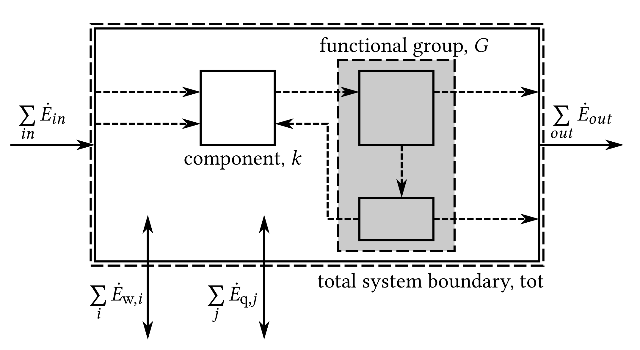
2.2. Exergy Analysis

Exergy is an extensive property giving information about the quantity and the thermodynamic quality of any energy carrier within an thermal conversion process. Consequently, only the exergy-based analysis enables comparability in evaluating material and energy flows of an overall plant or specific components [58].
The total exergy rate is the product of mass flow rate and specific exergy, which consists of the sum of physical e PH , chemical e CH , kinetic energy e KN , and potential exergy e PT . Effects associated with nuclear, magnetic, or electric processes are not considered [59].
E ˙ = m ˙ e PH + e CH + e KN + e PT
In the first step of implementing an exergy analysis in TESPy, only physical exergy will be considered.
e PH = h h 0 T 0 s s 0 = e T + e M
Furthermore, it is possible to split physical exergy into thermal and mechanical parts using the following Equations (4) and (5) [60]. In the first step, the fluid’s temperature is changed isobarically to the ambient temperature to obtain the thermal exergy. In the second step, the mechanical exergy is obtained by changing the fluid’s pressure isothermally to the ambient pressure.
e T = h h p , T 0 T 0 s s p , T 0
e M = h p , T 0 h p 0 , T 0 T 0 · s p , T 0 s p 0 , T 0
Thermal conversion processes are mainly open systems (see Figure 1). In addition to the energy flows of heat and work, there is also an exchange of material flows across the system boundary. The time-related change in the exergy within the overall system corresponds to the difference between all exergy flows entering and leaving the system, minus the exergy destruction caused by irreversibilities.
d E tot d t = j E ˙ q , j + i E ˙ w , i + i n E ˙ i n o u t E ˙ o u t E ˙ D
In the steady-state operation of a thermal conversion process, Equation (6) can be simplified.
0 = j E ˙ q , j + i E ˙ w , i + i n E ˙ i n o u t E ˙ o u t E ˙ D
The exergy destruction quantifies the thermodynamic inefficiencies associated with a process. These can be caused by chemical reaction, heat transfer, mixing, and friction and occur in every real system. The approach can thus be used to determine the components with the highest exergy destruction and the processes causing them [61].
For a single component k within the considered system, each term in Equation (7) can be assigned to the exergetic product or to the exergetic fuel [62]. The exergy destruction within the component is the difference of both terms.
E ˙ D , k = E ˙ F , k E ˙ P , k
The exergy efficiency of a component k is the ratio [63]:
ε k = E ˙ P , k E ˙ F , k
The sum of the exergy destruction in all components is equal to the exergy destruction of the total system. In addition, unused flows across the system boundary can be taken into account as exergy loss of the overall system.
E ˙ F , tot = E ˙ P , tot + E ˙ D , tot + E ˙ L , tot
Finally, the exergy efficiency of the overall system is defined as:
ε tot = E ˙ P , tot E ˙ F , tot = 1 E ˙ D , tot + E ˙ L , tot E ˙ F , tot
Based on the information from the overall system, the exergy destruction ratios for a component can be determined.
y D , k = E ˙ D , k E ˙ F , tot
y D , k * = E ˙ D , k E ˙ D , tot
Especially for larger systems with many components, it might be reasonable to aggregate several components into functional groups for improved readability of the analysis results. A functional group G consists of one or more components of the system, e.g., a steam generator, which composes of an economizer, a steam drum, an evaporator, and a superheater. In contrast to individual components, fuel and product exergy definitions cannot be made for generic functional groups. Therefore, instead of E ˙ F and E ˙ P , the sum of exergy carried into a functional group E ˙ in , G and the sum of exergy carried out of a functional group E ˙ out , G are used. The difference between these two values must then be the total exergy destruction of the functional group E ˙ D , G . This value must also be equal to the sum of exergy destruction values of all components g within that functional group (Equation (14)). Therefore, the exergy destruction ratios of a functional group y D , G and y D , G * can be calculated analogously as shown in Equations (12) and (13).
E ˙ D , G = g E ˙ D , g

2.3. Component-Based Thermodynamic Model

This section will formulate the equations used to model selected components of thermal conversion processes and the corresponding exergy balances. The full set of equations available for each component, as well as other components available in the software with their respective exergy balance equations, are documented in the API documentation [64].

2.3.1. Turbomachinery

All turbomachinery components, i.e., turbines, pumps, fans, and compressors, are considered to be adiabatic components. Therefore, the power transferred W ˙ can be calculated as the product of mass flow m ˙ and the change of enthalpy h between inlet (index in) and outlet (index out) of the component.
0 = W ˙ m ˙ · h out h in
The isentropic efficiency is a key figure of adiabatic turbomachinery. For a turbine, it describes the ratio of actual change in enthalpy to the theoretical maximum change in enthalpy of the isentropic process for a given change of pressure. The enthalpy at the outlet of the isentropic process h out , s is calculated from the outlet pressure and inlet entropy of that process (Equation (17)).
0 = η s , t · h out , s h in h out h in
h out , s = h p out , s p in , h in
The exergy balance of adiabatic expansion, therefore, is defined as follows. Three different cases are distinguished, depending on the ambient temperature in the exergy analysis [65].
E ˙ P = | W ˙ | T in , T out T 0 | W ˙ | + E ˙ out T T in > T 0 T out | W ˙ | + E ˙ out T E ˙ in T T 0 T in , T out
E ˙ F = E ˙ in PH E ˙ out PH T in , T out T 0 E ˙ in T + E ˙ in M E ˙ out M T in > T 0 T out E ˙ in M E ˙ out M T 0 T in , T out
Similar concepts apply to compression machines, e.g., pumps and compressors. However, in contrast to expansion, the isentropic efficiency is defined reciprocally.
0 = η s , c · h out h in h out , s h in
The exergy balance equations are similar to expansion processes as well. The compression machine draws power instead of supplying it.
E ˙ P = E ˙ out PH E ˙ in PH T in , T out T 0 E ˙ out T + E ˙ out M E ˙ in M T out > T 0 T in E ˙ out M E ˙ in M T 0 T in , T out
E ˙ F = | W ˙ | T in , T out T 0 | W ˙ | + E ˙ in T T out > T 0 T in | W ˙ | + E ˙ in T E ˙ out T T 0 T in , T out
An essential component of thermal processes is a multistage steam turbine with intermediate steam extraction for feedwater preheating. Such components can be modeled using multiple turbine parts connected to each other with splitters between one part and the next. Therefore, it is assumed that the entire mass flow of steam leaves a turbine part before entering the next one.

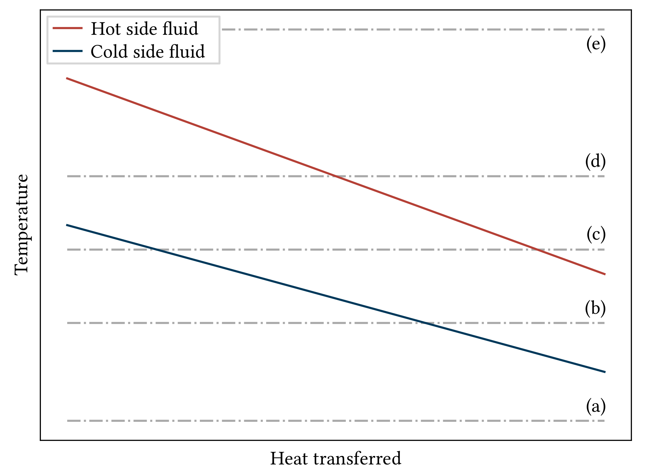
2.3.2. Heat Exchangers

Heat exchangers do only transfer heat. Heat losses to the ambient are neglected. The heat provided by the hot side (index 1) of a heat exchanger is therefore fully transferred to the fluid on the cold side (index 2) (Equation (23)). The heat transferred Q ˙ is calculated using Equation (24).
0 = m ˙ in , 1 · h out , 1 h in , 1 m ˙ in , 2 · h out , 2 h in , 2
0 = Q ˙ m ˙ in , 1 · h out , 1 h in , 1
Regarding the exergy balance of heat exchangers, it is necessary to distinguish six cases. Five cases are illustrated in Figure 2. The sixth variant is denoted as a purely “dissipative” heat exchanger regarding exergy, as the hot side of the heat exchanger is cooled toward T 0 while the cold side is heated towards T 0 , but T 0 is not crossed. While this type of heat exchanger has no exergetic product, it might be necessary to implement such a component for economic or technical reasons.
E ˙ P = E ˙ out , 2 T E ˙ in , 2 T ( a ) T in , 1 , T in , 2 , T out , 1 , T out , 2 > T 0 E ˙ out , 2 T ( b ) T in , 1 , T out , 1 , T out , 2 T 0 > T in , 2 E ˙ out , 1 T + E ˙ out , 2 T ( c ) T in , 1 , T out , 2 > T 0 T in , 2 , T out , 1 E ˙ out , 1 T ( d ) T in , 1 > T 0 T in , 2 , T out , 1 , T out , 2 E ˙ out , 1 T E ˙ in , 1 T ( e ) T 0 T in , 1 , T in , 2 , T out , 1 , T out , 2 not defined ( f ) T in , 1 , T out , 1 > T 0 T in , 2 , T out , 2
E ˙ F = E ˙ in , 1 PH E ˙ out , 1 PH + E ˙ in , 2 M E ˙ out , 2 M ( a ) T in , 1 , T in , 2 , T out , 1 , T out , 2 > T 0 E ˙ in , 1 PH E ˙ out , 1 PH + E ˙ in , 2 PH E ˙ out , 2 M ( b ) T in , 1 , T out , 1 , T out , 2 T 0 > T in , 2 E ˙ in , 1 PH + E ˙ in , 2 PH E ˙ out , 1 M E ˙ out , 2 M ( c ) T in , 1 , T out , 2 > T 0 T in , 2 , T out , 1 E ˙ in , 1 PH + E ˙ in , 2 PH E ˙ out , 2 PH E ˙ out , 1 M ( d ) T in , 1 > T 0 T in , 2 , T out , 1 , T out , 2 E ˙ in , 2 PH E ˙ out , 2 PH + E ˙ in , 1 M E ˙ out , 1 M ( e ) T 0 T in , 1 , T in , 2 , T out , 1 , T out , 2 E ˙ in , 1 PH E ˙ out , 1 PH + E ˙ in , 2 PH E ˙ out , 2 PH ( f ) T in , 1 , T out , 1 > T 0 T in , 2 , T out , 2
In addition to the energy and exergy balances, essential parameters for the design of heat exchangers are the terminal temperature difference values defining the temperature difference between the fluid on the hot side and the fluid on the cold side when entering and leaving the component. In TESPy, all heat exchangers implemented are countercurrent heat exchangers. The hot side inlet temperature difference Δ T in describes the temperature difference of the fluid entering the hot side to the fluid leaving on the cold side (Equation (27)). Similarly, the hot side outlet temperature difference Δ T out is the temperature difference of the fluid leaving the component on the hot side to the fluid entering on the cold side in Equation (28).
0 = Δ T in T p in , 1 , h in , 1 + T p out , 2 , h out , 2
0 = Δ T out T p out , 1 , h out , 1 + T p in , 2 , h in , 2
For condensers, i.e., heat exchangers with the purpose of condensing a fluid, there are two modifications applied. The condensing fluid on the hot side of the heat exchanger leaves the component as saturated liquid, i.e., the vapor mass fraction x equals zero (Equation (29)). The hot side inlet temperature difference is often referred to as terminal temperature difference, which uses the saturation temperature at the hot side inlet instead of the actual temperature in case the fluid enters the component as superheated vapor (Equation (30)). This is done because the enthalpy difference during desuperheating is much lower than during condensation. This also ensures that the cold side temperature can never be higher than the temperature of the condensing fluid in the model.
0 = h out , 1 h p out , 1 , x = 0
0 = Δ T in T sat p in , 1 + T out , 2
Last, the approach point temperature difference (Equation (31)) is an essential parameter. It describes the temperature difference to the boiling point Δ T ap of the working fluid for some heat exchangers, e.g., feedwater preheaters. In the economizer, it describes the temperature difference between vaporization temperature in the steam drum and the final preheating temperature and is thus crucial in the design to avoid evaporation in the economizer.
0 = T sat p Δ T ap T ap

2.3.3. Energy Balance Closing Components

In many applications, it might be useful to have a component closing the energy balance for the overall system, e.g., the solar field of a solar thermal power plant, as it effectively serves as energy input without necessarily needing information about the secondary side of the component. Therefore, the energy balance (Equation (32)) is applied. Other examples for this component might be heat losses in pipelines or solar-thermal collectors.
0 = Q ˙ m ˙ · h out h in
The exergy balance is related to the exergy balance of the heat exchanger but needs to distinguish between heat input and heat output:
E ˙ P = not defined if dissipative E ˙ in T E ˙ out T else T in , T out T 0 E ˙ out T T in T 0 > T out E ˙ out T E ˙ in T T 0 T in , T out Q ˙ < 0 E ˙ out PH E ˙ in PH T in , T out T 0 E ˙ in T + E ˙ out T T out > T 0 T in E ˙ in T E ˙ out T + E ˙ out M E ˙ in M T 0 T in , T out Q ˙ > 0
E ˙ F = E ˙ in PH E ˙ out PH T in , T out T 0 E ˙ in T + E ˙ in M + E ˙ out T E ˙ out M T in T 0 > T out E ˙ out T E ˙ in T + E ˙ in M E ˙ out M T 0 T in , T out Q ˙ < 0 E ˙ out T E ˙ in T T in , T out T 0 E ˙ in T + E ˙ in M E ˙ out M T out > T 0 T in E ˙ in T E ˙ out T T 0 T in , T out Q ˙ > 0

2.3.4. Merge Points

Another important component is the merge in which two or more different incoming streams (indexed i) are mixed with no transport of heat or power to the surroundings. Therefore, the energy balance equation can be deducted.
0 = i m ˙ in , i · h in , i m ˙ out · h out i inlets
The exergy balance equations are defined with the analogous approach of the heat exchanger exergy balance equations. For a mixing temperature T out higher than the ambient temperature, the product is heating the colder fluids. For a mixing temperature below the ambient temperature level, the product is cooling the hotter fluids. In addition, a distinction must be made in case an incoming stream is heated starting below the ambient temperature or cooled starting above the ambient temperature. In these cases, only change of exergy starting at the ambient temperature is accounted for in the product exergy (Equation (36)). The fuel exergy is then defined analogously (Equation (37)). If the temperature of the mixed stream is at ambient temperature, the component is considered a dissipative one. In the current version of the software TESPy, it is assumed that all mixed streams have the same chemical composition. Therefore, chemical exergies are not considered. Equations (36) and (37) cover all possible cases. It should be noted, however, that some of them are thermodynamically not meaningful.
E ˙ P = i m ˙ i · e out PH e in , i PH T in , i < T out & T in , i T 0 i m ˙ i · e out PH T in , i < T out & T in , i < T 0 T out > T 0 not defined T out = T 0 i m ˙ i · e out PH T in , i > T out & T in , i T 0 i m ˙ i · e out PH e in , i PH T in , i > T out & T in , i < T 0 T out < T 0
E ˙ F = i m ˙ i · e in , i PH e out PH T in , i > T out i E ˙ in , i PH T in , i < T out & T in , i < T 0 T out > T 0 i E ˙ in , i PH T out = T 0 i E ˙ in , i PH T in , i > T out & T in , i T 0 i m ˙ i · e in , i PH e out PH T in , i < T out T out < T 0

2.3.5. Steam Drum

A drum is implemented to separate saturated liquid from saturated vapor in the evaporation process. The drum’s energy balance is similar to that of a merge point with two streams leaving the device. Additional constraints are applied, i.e., the saturated liquid state at the first outlet stream and the saturated vapor state at the second outlet stream. Note that blowdown is not be considered in this modeling approach.
0 = i m ˙ in , i · h in , i j m ˙ out , j · h out , j
0 = h out , 1 h p out , 1 0 = h out , 2 h p out , 2
It is usually not meaningful to define an exergy efficiency just for a steam drum alone, since this component is part of an evaporator.

2.3.6. Motors and Generators

The turbines of the plant power a generator, whereas pumps and fans require an electrical motor to be powered. Assuming an efficiency for the generator η el , m , its electrical power output of a generator W ˙ el , gen is calculated according to Equation (40). The turbine power W ˙ (Equation (15)) is multiplied with the efficiency factor η el , m considering mechanical and electrical losses.
W ˙ el , gen = W ˙ · η el , m
Analogously, in Equation (41), the electrical power input for a motor W ˙ el , mot is determined.
W ˙ el , mot = W ˙ η el , m

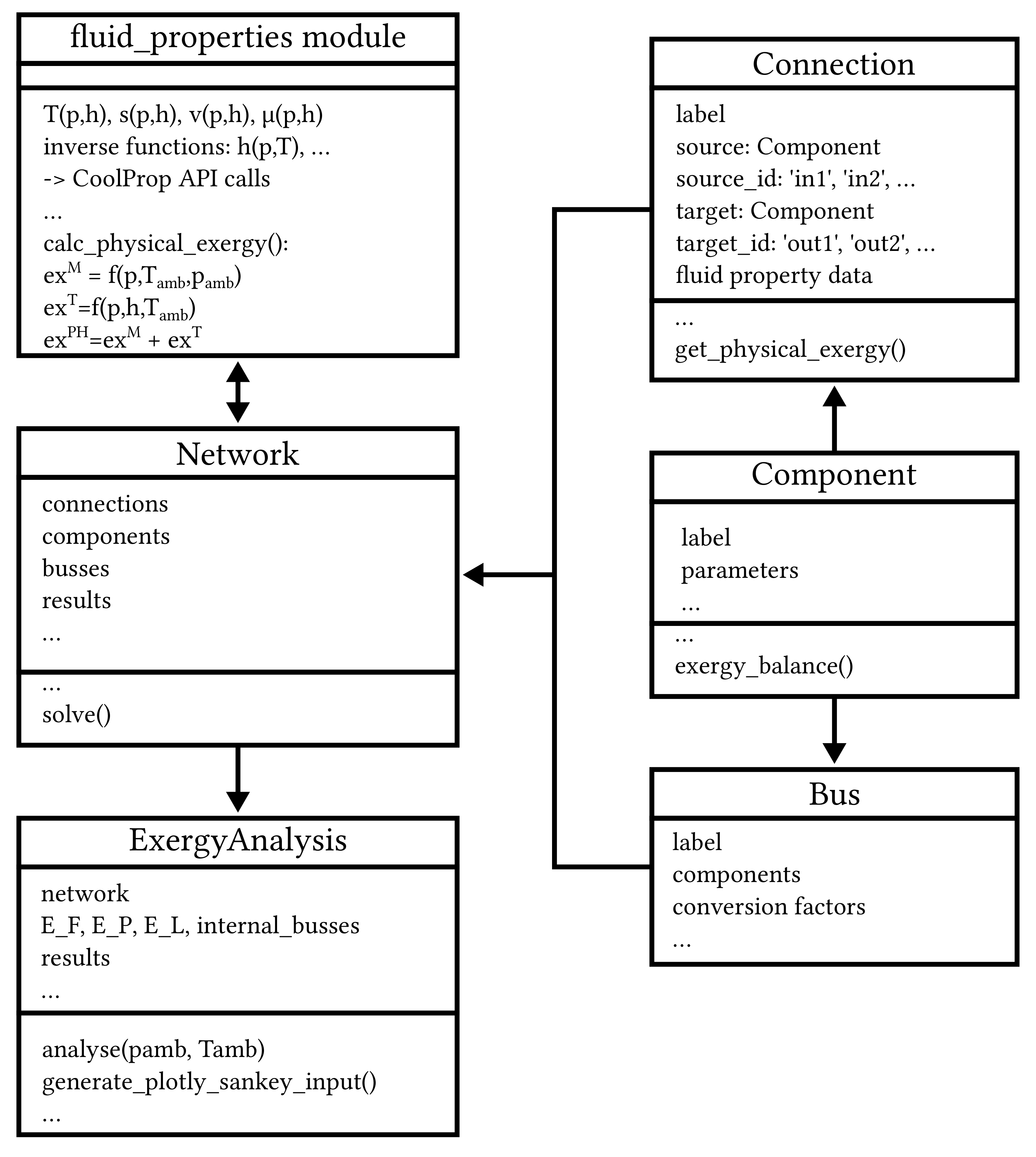
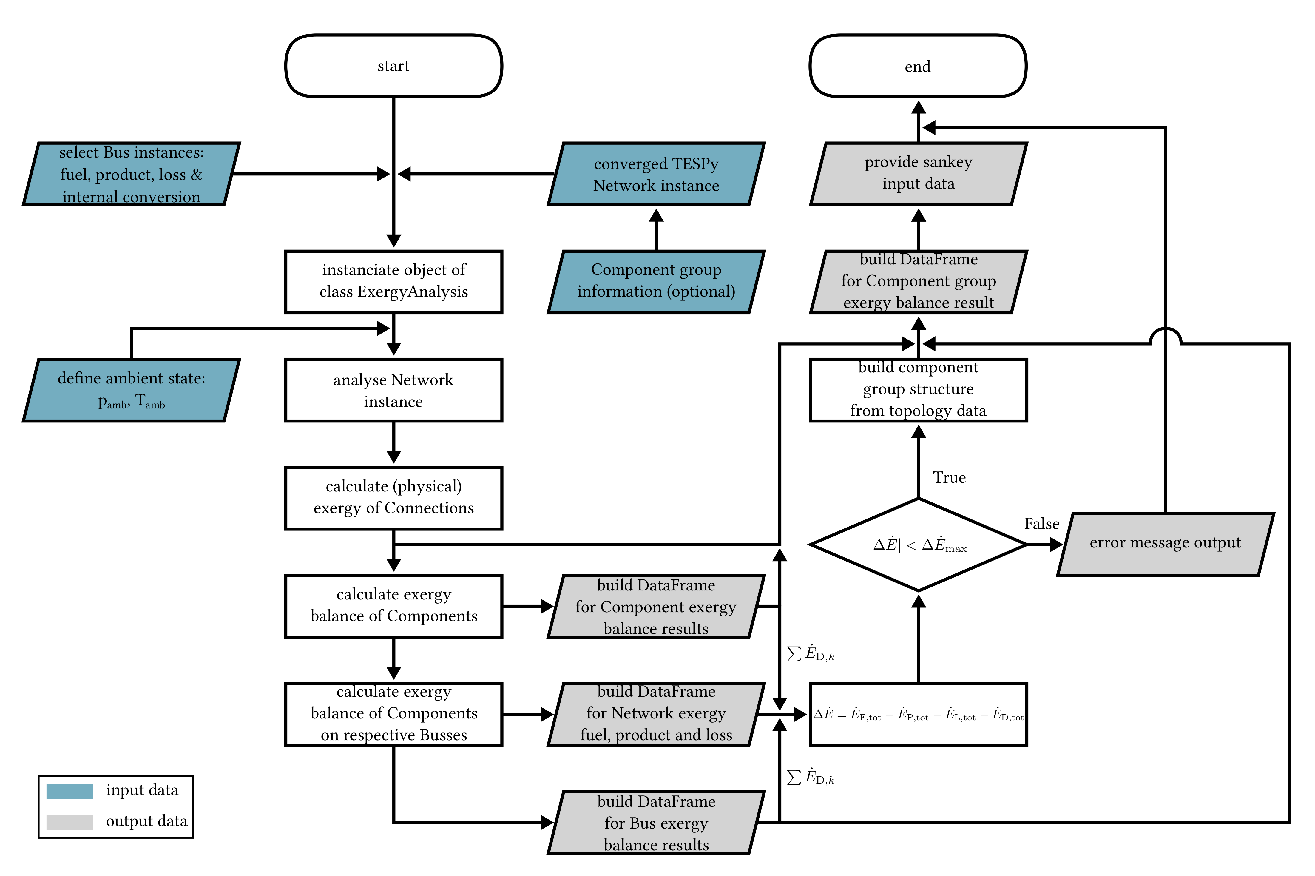
3. Implementation of the Exergy Analysis in TESPy

Here, the implementation of a generic exergy analysis is presented. The software TESPy is designed to simulate the steady-state operation of thermal conversion processes, such as thermal power plants, heat pumps, or pipeline networks at the component level. The software models typical units (e.g., turbines, pumps, heat exchangers), thus allowing the user to build generic plant models [66]. An introduction to Python fundamentals is given in [67].
Figure 3 shows an overview of the structure of TESPy. Each simulation model is based inside the network class. The class automatically builds a system of nonlinear equations representing the plant’s topology and the boundary conditions specified, for instance, cooling water temperature or turbine isentropic efficiency. The topology is derived from the connections between the system’s components. Therefore, the connection class holds the topological information by connecting a source component with a target component and the fluid property data, i.e., mass flow, pressure, enthalpy, and mass fraction. In addition, it is possible to connect pure energy streams, e.g., the power of a turbine or the power of a pump, by the use of energy busses (class bus). Conversion losses can be considered with constant efficiency values.
The system of equations is solved numerically with the multidimensional Newton-Raphson algorithm for the system’s variables, which are mass flow, pressure, enthalpy, and fluid mass fraction on every connection. As mass flow and fluid property data are available for all connections after a converged simulation is obtained, all remaining variables of a stream, e.g., pressure or temperature, and all component parameters, can be determined with the fluid property module. The module holds all functions to calculate required fluid properties, including calculation of physical exergy using CoolProp [68]. The online documentation provides extensive information on the component models and fluid property calculations applied in the software.
Figure 4 illustrates the procedure of the exergy analysis implemented in TESPy. The user defines the busses of the TESPy network, which hold information on fuel and product exergy and exergy loss. These are passed together with the network to create an instance of the class ExergyAnalysis (see also Figure 3). Subsequently, the exergy analysis is carried out using data of the ambient state, i.e., pressure and temperature. In the first step, physical exergy, including thermal and mechanical exergy (see Equations (5) and (4)) of all fluid streams, is calculated for the connection objects of the network. In the second step, the exergy balance of all components (see Section 2.3) is evaluated.
Based on the exergy balances of the components, the exergy balances of the busses corresponding to the plant’s total fuel and product exergy and exergy loss are evaluated. Furthermore, the balance equations for internal massless exergy transfer, e.g., a feed pump that is directly driven by a respective turbine, are calculated. The individual conversion factor of each component as part of a bus object is applied to the exergy flow, analogously to the definition of generator and motor power in Equations (40) and (41). The exergy destruction within each component and their corresponding bus (if any) is summed to calculate the network’s total exergy destruction E ˙ D , tot . As all elements of the overall network exergy balance are now known (Equation (10)), a consistency check can be carried out, where the deviation Δ E of total fuel exergy E ˙ F , tot from the sum of total product exergy E ˙ P , tot , exergy loss E ˙ L , tot , and exergy destruction E ˙ D , tot must be equal to zero. To account for rounding errors, the absolute value of Δ E ˙ should be smaller than a threshold value of 0.001 W. When running the exergy analysis on a converged simulation, this condition must be true. If it is not, some exergy streams in the overall system have not correctly been accounted for in the exergy analysis setup.
Finally, all exergy balance data of the components and their respective busses, including exergy efficiency as well as exergy destruction and exergy loss ratio, are provided to the user as pandas DataFrames [69], which can easily be exported to any tabular format. Furthermore, the physical exergy values of all connections are accessible in a DataFrame.
In addition, during the setup of the system’s components, the user can assign each component to a functional group, as described in Section 2.2. A DataFrame is then provided for all functional groups, including their information on the inflow E ˙ in , G and outflow of exergy E ˙ out , G , the total exergy destruction as well as the exergy destruction ratios according to their definitions in Equations (7) and (12)–(14). If a component is not assigned to any functional group, it will form a functional group by itself. With these data, a graphical representation of exergy flows between the different functional groups of the system in a Grassmann diagram [70] is enabled. For this purpose, the data is provided as expected by the Python library plotly for its Sankey class [71]. The functional groups, including individual components, that form their own functional group, are the nodes of the Grassmann diagram. The edges represent the exergy flows. The values are shown in a true-to-scale manner by the width of the edges. The exergy flows of the overall system across the system boundary (see Equation (10)) are each represented by their respective color. Exergy flows associated with a mass flow of a fluid, a heat rate, or work rate within the system boundary are marked with a unique color. The software provides default color codes; however, the user can specify the colors as desired. For more information, please visit the respective section of the online documentation [64]. The diagram is provided in an interactive format, showing additional information when hovering over nodes and edges. The displayed data can be modified according to the user’s requirements following the API of plotly.
Given the exergy streams crossing the system’s boundaries are well defined by the user, changing any values in the process’s specifications or even modifying the plant’s topology does not require any changes regarding the exergy analysis setup. The analysis can be performed again easily. The online documentation of TESPy provides several examples on the usage and implementation of the exergy analysis as well.

4. Example Applications

Exergy analyses are carried out for three different applications to demonstrate the new feature in TESPy. The Python scripts, the result reports, and the model validation are available via zenodo.
  • The so-called “Solar Energy Generating System VI” (SEGS) [72], see Section 4.1
  • Supercritical CO2 power cycle [73], see Section 4.2
  • Refrigeration machine using air as working fluid [74], see Section 4.3
Subsequently, the examples are briefly presented with the respective results generated by the exergy analysis tool. The SEGS model is validated using the proprietary software Ebsilon. The other two examples have originally been published in [75,76]. These contain all data necessary to set up and evaluate the TESPy simulation. Therefore, the respective TESPy models are compared to results from these publications instead of using Ebsilon. The versions used are TESPy v0.6.0 [77] and Ebsilon 14.03.01.

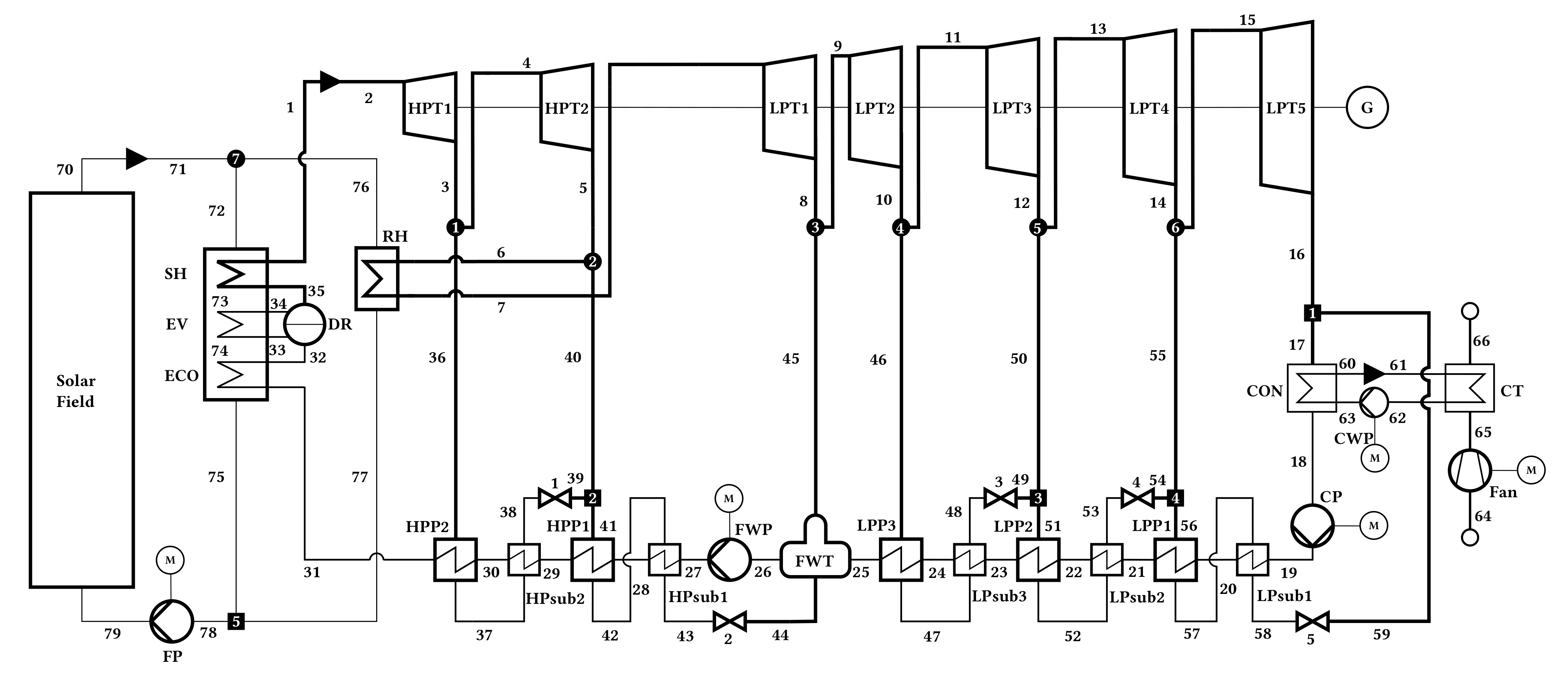
4.1. Solar Energy Generating System

The SEGS in Southern California, USA, has been chosen as a real application. A complete set of parameters and performance data is available in References [78,79] for this concentrating solar power (CSP) plant.

4.1.1. Process Simulation and Validation

SEGS consists of three major subsystems: the solar field, the power cycle, and the cooling water system. The TESPy model corresponds to the layout shown in Figure 5.
In the first subsystem, a eutectic mixture of diphenyl oxide and biphenyl, commercially known as Therminol VP-1 [80], circulates as the heat transferring fluid (HTF). The heat rate from the solar field is transferred through the heat exchangers of the steam generator and the reheater to the power cycle. In the steam generator, the HTF is split into two parallel heat exchanger trains. Each consists of a superheater, evaporator, and economizer. The division into two parallel streams also applies to the reheater. For simplicity, the two trains are modeled as a single one in both cases. A field pump ensures the circulation of the HTF. The solar field is modeled as simple heat input. The exact layout of the solar field does not influence the overall analysis.
The steam turbine drives the generator to provide electricity. The steam turbine is divided into a high-pressure and a low-pressure turbine. In between, reheating is used. The turbine sections are split into two and five parts to extract steam for preheating, respectively. The power plant has three low-pressure and two high-pressure preheaters and a feedwater tank (deaerator).
An induced draft cooling tower is used for recooling. Therefore, a cooling water cycle is modeled, transporting the heat rate from the power cycle via a heat exchanger to the ambient air. A fan provides the necessary mass flow rate of air.
The example covers the design state in full-load steady-state conditions and pure solar mode. Table 2 summarizes selected process and component parameters. For a complete set of input parameters, see model documentation in [72].
The isentropic efficiencies of the turbines are taken from [81], which are derived them from the stated properties for every stream in [78]. Due to inconsistencies in the primary data, a reasonable isentropic efficiency for the fourth low-pressure turbine stage of 88% was assumed.
Regarding the preheaters, the pressure drop on the hot side is neglected. The pressure drop on the cold side has been calculated by using the stated properties for every stream in [78]. This procedure has also been applied to the steam generator and reheater. The temperature difference for the approach point in the steam generator is assumed to be 2 K, and the pinch point temperature difference is at 5 K. Regarding the temperature specifications of the preheaters and the steam generator, the assumptions listed in Table 2 have been applied.
Table 2. SEGS—Parameters of the overall process and components [78,82].
ParameterSymbolUnitValue
HTF temperature T 70 C 390
HTF mass flow ratio m ˙ 76 / m ˙ 70 -0.13
Steam temperatures T 1 , T 7 C 371, 371
Steam pressures p 1 , p 7 bar 100, 17.1
Steam mass flow m ˙ 1 kg / s 38.97
Condensation pressure p 17 bar0.08
Pumps, efficiencies η is , η el , m %70.0, 95.0
Generator, efficiency η el , m %97.0
Air fan, efficiency η is %60.0
Preheaters, upper temperature difference Δ T t , u K 5
Subcoolers, lower temperature difference Δ T t , l K 10
Pressure losses during the condensation on the hot side of the condenser are neglected. For the cooling system, the parasitic power requirement is at 0.91 MW [78]. Therefore, an air cooling tower is implemented to cool the water in an intermediate cycle for the main condenser of the power plant. With the assumptions made in the simulation, the parasitic power requirements for the cooling system add up to 0.92 MW.
In addition to the TESPy model, an identical model has been built with the industrial standard software Ebsilon. As TESPy’s thermodynamic library for fluid property calculation CoolProp [68] is available for Ebsilon as well, it is used in both models. The library contains Therminol VP-1 as an incompressible liquid, the air is calculated as pseudopure fluid with the Helmholtz equation of state (HEOS) back-end, and for water, the IAPWS-95 formulation is implemented. The results obtained from both models are identical.

4.1.2. Results of the Exergy Analysis

The exergy-based analysis is carried out for the specifications used in the model validation. The ambient temperature T 0 is 25 C ; the ambient pressure p 0 is 1.013 bar.
Table 3 shows the exergy balance of the overall process for SEGS. The product exergy corresponds to net power output. If the energy rate absorbed by the parabolic trough collectors is specified as the exergetic fuel, this results in an exergy efficiency ε tot of 66.7% for the overall process. The real thermodynamic losses at the solar field, i.e., the difference between the exergy of the incident global radiation and the exergy associated with the absorbed heat rate, are thus not taken into account. The overall exergy loss E ˙ L , tot is the release of the cooling air to the environment. Compared to the overall exergy destruction, the overall exergy loss is significantly smaller since the temperature of the released air, and thus the physical exergy of the material flow, is low.
The power plant simulation model consists of a large number of individual components. For a better understanding of the causes of exergy destruction, components were accumulated into functional groups. Results are presented in Table 4. Based on these results, the Grassmann diagram feature of TESPy can be used to create Figure 6, which illustrates the flow of exergy through the functional groups.
It can be seen that the low-pressure turbine (LPT) and the cooling water system (CW) account for almost 50% of the overall exergy destruction rate. Especially the low value of isentropic efficiency of the low-pressure turbine causes a high share of exergy destruction. For the cooling water system, only the condensate is reused within the plant, which is close to the ambient state. Therefore, most of the exergy is destroyed or lost to the ambient state. Other quantitatively relevant contributions to the overall exergy destruction rate occur in the steam generator (SG) and the high-pressure turbine (HPT). All other functional groups account for less than 10% each, summing up to approx 24% in total.

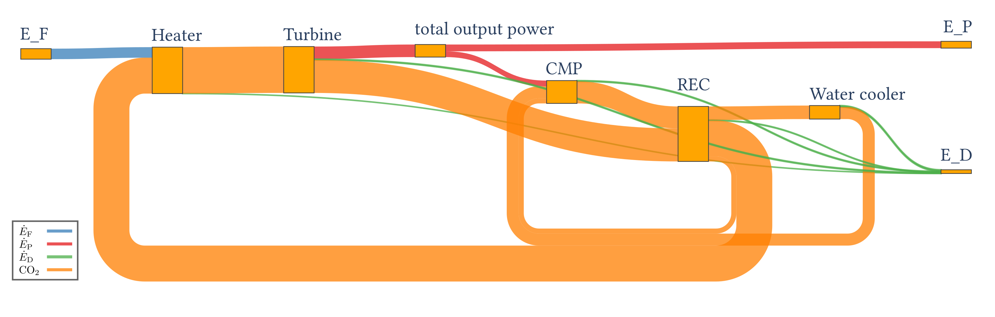
4.2. Supercritical Carbon Dioxide Power Cycle

As a second example, the variant c) of the supercritical CO2 (sCO2) power cycles reported by Penkuhn and Tsatsaronis [75] has been implemented and analyzed using TESPy as all necessary input data, and the results of the exergy-based analysis are available.

4.2.1. Process Simulation and Validation

The investigated cycle is the recompression, recuperated cycle, with two compressors and one turbine. The working fluid is heated and routed to the turbine. After expansion, two recuperators are used to preheat the compressed CO2. After exiting the recuperators, one part of the fluid is cooled and compressed before entering the cold side of the recuperator 1. The remaining CO2 is compressed without entering the cooler and mixed into the reheated CO2 stream from the first compressor and then routed through the recuperator 2 before entering the heater. The model created in TESPy corresponds to the layout shown in Figure 7.
In contrast to the original study, the exergy balances of the heater and the cooler are modeled without knowledge of the temperature profile of the non-CO2 side (see Section 2.3.3). The cooler is considered a dissipative component. Thus, the plant will not have exergy losses. Furthermore, the distribution of the mass flow through compressor 1 and compressor 2 is assumed to be a result of the temperature values observed at the merge point between the recuperators. The compressor 2 and recuperator 1 outlet temperatures T 11 and T 12 are thus specified to be equal (but unknown prior to the calculation) values. Table 5 summarizes selected process and component parameters. For a complete set of input parameters, see model documentation [73].
In this example, HEOS back-end of CoolProp was used as well. Although the data from the original source are based on the REFPROP database and calculation, the relative deviation between both libraries is less than 10 9 for enthalpy values and 10 12 for entropy values. Consequently, the results agree except for numerical deviations without impacting real-life operation. The highest deviation in thermodynamic properties is observed in the turbine outlet temperature T 5 with 0.2 K. All other (nonspecified) temperature values are within less than 0.1 K compared to the original data. Therefore, a deviation can be observed in the physical exergy of the streams. Considering the overall cycle efficiency η th , a relative deviation of about 0.1% occurs.

4.2.2. Results of the Exergy Analysis

The exergy-based analysis is carried out for an ambient temperature T 0 of 25 C and an ambient pressure p 0 of 1.013 bar. The results of the analysis are summarized in Table 6 and Table 7. Since the number of components in this application is low, the component results are reported instead of the functional group results. The net power generation of the process is associated with the product exergy E ˙ P , tot . If the exergy rate supplied to the process associated with the heat rate is considered as fuel exergy E ˙ F , tot , the overall exergy efficiency ε tot is 64.6%. Figure 8 illustrates the exergy flow rates within the process.
The highest share of the overall exergy destruction rate can be observed in the cooler. The exergy destruction rate of the rotating equipment—compressors and turbine—amounts to a cumulative 24 MW. The heater has the smallest share in the total exergy destruction rate, as per definition in Equations (33) and (34) only the pressure losses account for the exergy destruction rate in this type of heat exchanger. Note that the difference in the definition of the heater’s exergy balance is the reason why a high relative deviation in the exergy destruction values between the results of this paper and the original study (approx. −70%) is observed.

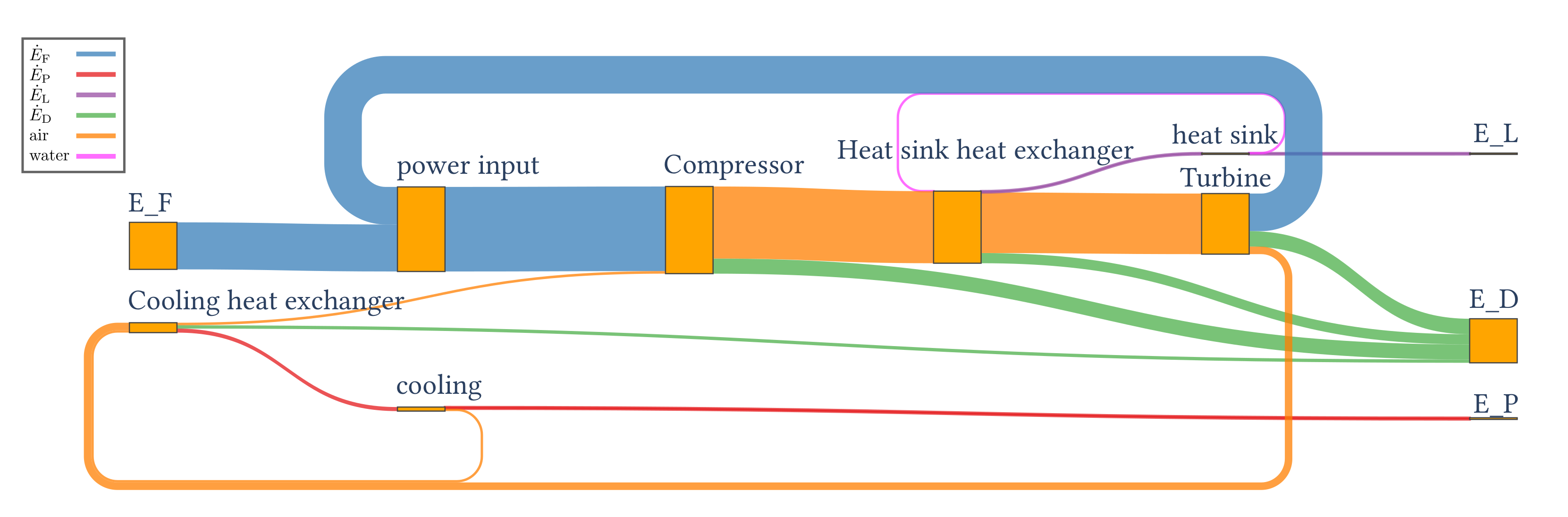
4.3. Air Refrigeration Cycle

The third example focuses on a refrigeration cycle using air as working fluid originally presented by Morosuk and Tsatsaronis [76].

4.3.1. Process Simulation and Validation

The process consists of a four-component refrigeration cycle with compressor, heater, cooler, and turbine. The compressor and turbine are on a single shaft, and an inverter is included in the original analysis to account for conversion losses of the electrical power input to mechanical power of the shaft driving the compressor, as seen in Figure 9. The cycle is applied to cool air. The heat sink is water at ambient conditions.
Table 8 summarizes selected process and component parameters. For a complete set of input parameters, see model documentation [74]. The input data match the original data from [76]. However, due to the architecture of the TESPy solver and the exergy analysis feature, losses on a single shaft with respect to the residual power W ˙ cmp + W ˙ tur cannot be accounted in the same way as in the original study. Therefore, the residual power is first determined without accounting for losses.
W ˙ cmp + W ˙ tur η el , original = W ˙ cmp η el , m + W ˙ tur · η el , m
In a second step, equal efficiencies η el , m for both, the turbine’s generator and the compressor’s motor, are applied to the power bus to match the efficiency specifications of the original study η el , original = 0.9 (see Equation (42)). This results in an efficiency η el , m of 96.2%.
For the original analysis, the used fluid property back-end is not documented. In the TESPy model, the HEOS for pseudopure dry air is applied using CoolProp. Deviations in the outlet temperature of the compressor and the turbine of 0.04% and −0.18%, respectively, can be observed. A relatively high deviation is found in the enthalpy difference at the cooling side heat exchanger with about 2%. For the other components, the maximum deviation is at the heat sink heat exchanger with about 0.6% and 0.55% on the secondary stream of the cooling heat exchanger. Due to the 2% deviation, the cycle’s mass flows calculated with the TESPy model deviate by the same value as the governing equation for mass flow is the heat transferred at that heat exchanger (see Equation (23)).

4.3.2. Results of the Exergy Analysis

The ambient state is not explicitly reported in the original study but can be derived from the exergy tables. The ambient temperature T 0 is 25 C ; the ambient pressure is 1.0 bar.
Overall, the specific thermal exergy data of the streams are consistent with the reported data from literature. The mechanical exergy matches for all streams, as all pressure values are identical. The deviations in the thermodynamic properties, including the exergy values between the original paper and the calculations reported here, are lower than 2.1% and are caused by the different fluid properties functions used in each calculation. Since the inverter is treated separately in the original study, high deviations are observed in the compressor and turbine exergy analysis results.
The results of the exergy analysis are presented in Table 9 and Table 10. The total product exergy is associated with the exergy rate required to cool the air. The total fuel exergy represents the power input. This results in an overall exergy efficiency of 3.5%.
The compressor, the turbine, and the heat sink heat exchanger have the highest shares of the overall exergy destruction rate, with 92.5%. This includes the mechanical losses on the shaft, which account for 10.7% of the overall exergy destruction rate. The heat sink heat exchanger has the smallest share of the overall exergy destruction rate. Figure 10 illustrates the exergy flow rates within the process.

5. Conclusions

Exergy-based analyses are powerful tools for the thermodynamic and thermoeconomic investigation of thermal conversion processes. Available simulation and analysis software, proprietary as well as free and open-source, do not provide a fully integrated solution for such analyses. Considering that such analysis requires knowledge of the topological structure of a process and the results from a respective simulation, it is evident that exergy-based analyses should be integrated as automatic analyses following the solution of the system of equations of the simulation.
For the first time, open-source software can perform a generic exergy analysis for thermal conversion processes. The automated exergy analysis allows evaluation for processes above, below, and with a transition at T 0 . The study provides exergy efficiencies for all possible application cases for all basic unit operations of thermal process engineering (for the heat exchanger, for example, see Equations (25) and (26)). Furthermore, Grassman diagrams can be generated.
The paper discussed the approach, summarized the equations and definitions used, and validated the results with three example applications. The contributions of our research can be summarized as follows.
  • A complete set of exergy balance equations, including definitions of fuel and product exergy, for the most important components in thermal conversion processes is implemented.
  • The paper presents a generic and reproducible workflow. It allows researchers to perform exergy analyses based on any thermodynamic application modeled by the software.
  • The thermodynamic models and the results of the exergy analysis have been validated based on published research.
  • Due to the fully integrated solution, changes in topology or parameter specifications of an existing model do not require changes in the exergy analysis setup.
  • Providing the results in modern data structures enables further investigation or integration of external algorithms, e.g., exergy-based optimization procedures. For instance, refs. [83,84] published implementations of optimization procedures using first law analysis with TESPy.
  • Updating and evaluating exergy analyses of published research is possible.
While the exergy analysis in the presented research as well as the software implementation do cover a wide range of thermal engineering applications, two important use cases for exergy analysis have not yet been considered, in addition to the inclusion of calculation of chemical exergies. These are:
  • Analysis of processes with conversion of matter, such as gas turbine power plants or power-to-gas facilities.
  • Provision of exergoeconomical analysis tools.
The next step in the further development of the software is the implementation of chemical exergy. Due to the modular structure, this step means to integrate the methods of chemical exergy calculation for every stream of matter and to update the exergy balance equations of the components to account for the change in chemical exergy. For the implementation of the exergoeconomic analysis, additional functionalities have to be added to the component classes to define cost balances and auxiliary equations.

Author Contributions

Conceptualization, F.W., M.H. and I.T.; methodology, F.W. and M.H.; software, F.W. and J.M.; validation, F.W. and I.T.; formal analysis, F.W. and J.M.; investigation, F.W., J.M. and M.H.; resources, M.H. and I.T.; data curation, F.W.; writing—original draft preparation, F.W., J.M. and M.H.; writing—review and editing, F.W., M.H., I.T. and G.T.; visualization, F.W., J.M. and M.H.; supervision, I.T. and G.T. All authors have read and agreed to the published version of the manuscript.

Funding

We acknowledge financial support by Land Schleswig-Holstein within the funding programme Open Access-Publikationsfonds.

Data Availability Statement

All models and data used are available (see [72,73,74]). If you want to report bugs use the respective Github repositories (see [85,86,87]). The software presented can be downloaded via [77]. An online documentation [64] is available too.

Acknowledgments

During writing this paper, a long-time employee of our department passed away suddenly and unexpectedly. Christine Gharz supported our scientific activities with great engagement for more than 25 years. George Tsatsaronis and Mathias Hofmann dedicate this article to her memory.

Conflicts of Interest

The authors declare no conflict of interest.

Nomenclature

Abbreviations
APIApplication programming interface
CMPCompressors
CONCondenser
CSPConcentrating solar power
CPCondensate pump
CTCooling tower
CWCooling water
CWPCooling water pump
ECOEconomizer
EOEquation-oriented
EVEvaporator
DRDrum
FPField pump
FWPFeed water pump
FWTFeed water tank
HEOSHelmholtz equation of state
HPPHigh-pressure preheater
HPTHigh-pressure turbine
HTFHeat-transfer fluid
IAPWSInternational Association for the Properties of Water and Steam
LPPLow-pressure preheater
LPTLow-pressure turbine
NISTNational Institute of Standards and Technology
RECRecuperators
RHReheater
sCO2supercritical CO2
SHSuperheater
SEGSSolar Energy Generating System
SGSteam generator
SMSequential-modular
subSubcooler
TESPyThermal Engineering Systems in Python
Latin symbols
m ˙ Mass flow, kg/s
cFlow velocity, m/s
E ˙ Exergy flow, W
gGravity, m/s²
hSpecific enthalpy, J/kg
pPressure, bar
Q ˙ Heat flow, W
sSpecific Entropy, J/kgK
TTemperature, C
W ˙ Power, W
xSteam mass fraction, -
yExergy destruction ratio, -
zHeight, m
Greek symbols
η Energetic efficiency
Δ Difference
ε Exergetic efficiency
Subscripts and superscripts
0Reference state
apApproach point
CHChemical
cmpCompressor
DDestruction
elElectrical
FFuel
ggth component of functional group
genGenerator
GFunctional group
inInlet
kkth component
KNKinetic
LLoss
mMechanical
MMechanical
minMinimum
motMotor
outOutlet
PProduct
PHPhysical
PTPotential
sIsentropic
satAt saturation
TThermal
totTotal
turTurbine

References

  1. McLeod, J. Simulation Is Wha-a-At. Simulation 1963, 1, 5–6. [Google Scholar] [CrossRef]
  2. Youle, P. H3. Simulation techniques in chemical reaction engineering. Chem. Eng. Sci. 1961, 14, 252–257. [Google Scholar] [CrossRef]
  3. Shubik, M. Simulation of the industry and the firm. Am. Econ. Rev. 1960, 50, 908–919. [Google Scholar]
  4. Motard, R.L.; Shacham, M.; Rosen, E.M. Steady state chemical process simulation. AIChE J. 1975, 21, 417–436. [Google Scholar] [CrossRef]
  5. Marquardt, W. Von der Prozeßsimulation zur Lebenszyklusmodellierung. Chem.-Ing.-Tech. 1999, 71, 1119–1137. (In German) [Google Scholar] [CrossRef]
  6. Walter, H.; Epple, B. (Eds.) Numerical Simulation of Power Plants and Firing Systems; Springer: Vienna, Austria, 2017. [Google Scholar] [CrossRef]
  7. Banks, J.; Carson, J.S.; Nelson, B.L.; Nicol, D.M. Discrete-Event System Simulation; Pearson: Upper Saddle River, NJ, USA, 2010. [Google Scholar]
  8. Westerberg, A.W.; Hutchison, H.P.; Motard, R.L.; Winter, P. Process Flowsheeting; Cambridge University Press: Cambridge, UK, 1979. [Google Scholar]
  9. Sinha, R.; Paredis, C.J.J.; Liang, V.C.; Khosla, P.K. Modeling and simulation methods for design of engineering systems. J. Comput. Inf. Sci. Eng. 2001, 1, 84–91. [Google Scholar] [CrossRef]
  10. Takamatsu, T. The nature and role of process systems engineering. Comput. Chem. Eng. 1983, 7, 203–218. [Google Scholar] [CrossRef]
  11. Zeigler, B.P. Object-Oriented Simulation with Hierarchical, Modular Models; Academic Press: San Diego, CA, USA, 1990. [Google Scholar]
  12. Marquardt, W. Towards a process modeling methodology. In Methods of Model Based Process Control; Berber, R., Ed.; Kluwer: Dordrecht, The Netherlands, 1995; pp. 3–40. [Google Scholar] [CrossRef]
  13. Schuler, H. (Ed.) Prozeßsimulation; VCH: Weinheim, Germany, 1995; (In German). [Google Scholar] [CrossRef]
  14. Stamatelopoulos, G.N. Berechnung und Optimierung von Kraftwerkskreisläufen; Fortschritt-Berichte 340, Reihe 6; VDI Verlag: Düsseldorf, Germany, 1996. (In German) [Google Scholar]
  15. Zoder, M.; Balke, J.; Hofmann, M.; Tsatsaronis, G. Simulation and exergy analysis of energy conversion processes using a free and open-source framework—Python based object-oriented programming for gas- and steam turbine cycles. Energies 2018, 11, 2609. [Google Scholar] [CrossRef] [Green Version]
  16. Miller, K.W.; Voas, J.; Costello, T. Free and Open Source Software. IT Prof. 2010, 12, 14–16. [Google Scholar] [CrossRef]
  17. Feller, J.; Fitzgerald, B.; Hissam, S.A.; Lakhani, K.R. (Eds.) Perspectives on Free and Open Source Software; MIT Press: Cambridge, MA, USA, 2005. [Google Scholar]
  18. Crowston, K.; Wei, K.; Howison, J.; Wiggins, A. Free/Libre open-source software development: What we know and what we do not know. ACM Comput. Surv. 2012, 44, 7:1–7:35. [Google Scholar] [CrossRef]
  19. Tsatsaronis, G. Thermoeconomic analysis and optimization of energy systems. Prog. Energ. Combust. 1993, 19, 227–257. [Google Scholar] [CrossRef]
  20. Giglmayr, I.E. Modellierung von Heiz- und Heizkraftwerken; Fortschritt-Berichte 470, Reihe 6; VDI Verlag: Düsseldorf, Germany, 2001. (In German) [Google Scholar]
  21. Martelli, E.; Alobaid, F.; Elsido, C. Design optimization and dynamic simulation of steam cycle power plants: A review. Front. Energy Res. 2021, 9, 676969. [Google Scholar] [CrossRef]
  22. Asprion, N.; Rumpf, B.; Gritsch, A. Work flow in process development for energy efficient processes. Appl. Therm. Eng. 2011, 31, 2067–2072. [Google Scholar] [CrossRef]
  23. Asprion, N.; Mollner, S.; Poth, N.; Rumpf, B. Energy Management in Chemical Industry. In Ullmann’s Encyclopedia of Industrial Chemistry; Wiley-VCH: Weinheim, Germany, 2010; pp. 501–520. [Google Scholar] [CrossRef]
  24. Morris, D.R.; Szargut, J. Standard chemical exergy of some elements and compounds on the planet earth. Energy 1986, 11, 733–755. [Google Scholar] [CrossRef]
  25. Szargut, J.; Morris, D.; Steward, F. Exergy Analysis of Thermal, Chemical, and Metallurgical Processes; Hemisphere: New York, NY, USA, 1988. [Google Scholar]
  26. Szargut, J. Chemical exergies of the elements. Appl. Energ. 1989, 32, 269–286. [Google Scholar] [CrossRef]
  27. Szargut, J.; Valero, A.; Stanek, W.; Valero, A. Towards an International Reference Environment of Chemical Exergy. In Proceedings of the ECOS, Trondheim, Norway, 20–22 June 2005; pp. 409–417. [Google Scholar]
  28. Szargut, J. Egzergia; Slesian University of Technology: Gliwice, Poland, 2007. (In Polish) [Google Scholar]
  29. Ahrendts, J. Die Exergie Chemisch Reaktionsfähiger Systeme; VDI-Forsch.-Heft 579; VDI Verlag: Düsseldorf, Germany, 1977. (In German) [Google Scholar]
  30. Ahrendts, J. Reference states. Energy 1980, 5, 666–677. [Google Scholar] [CrossRef]
  31. Kameyama, H.; Yoshida, K.; Yamauchi, S.; Fueki, K. Evaluation of reference exergies for the elements. Appl. Energ. 1982, 11, 69–83. [Google Scholar] [CrossRef]
  32. Van Gool, W. Thermodynamics of chemical references for exergy analysis. Energ. Convers. Manage. 1998, 39, 1719–1728. [Google Scholar] [CrossRef]
  33. Diederichsen, C. Referenzumgebungen zur Berechnung der Chemischen Exergie; Fortschritt-Berichte 50, Reihe 19; VDI Verlag: Düsseldorf, Germany, 1991. (In German) [Google Scholar]
  34. Shieh, J.H.; Fan, L.T. Estimation of Energy (Enthalpy) and Exergy (Availability) Contents in Structurally Complicated Materials. Energy Sources 1982, 6, 1–46. [Google Scholar] [CrossRef]
  35. Stepanov, V.S. Chemical Energies and Exergies of Fuels, 2nd ed.; Nauka: Novosibirsk, Russia, 1990. (In Russian) [Google Scholar]
  36. Stepanov, V.S. Chemical energies and exergies of fuels. Energy 1995, 20, 235–242. [Google Scholar] [CrossRef]
  37. Fratzscher, W.; Michalek, K.; Szargut, J. Unterschiedliche Bezugssysteme zur Berechnung der chemischen Exergie. Chem. Tech. 1989, 41, 321–327. (In German) [Google Scholar]
  38. Rosen, M.A.; Scott, D.S. The enhancement of a process simulator for complete energy-exergy analysis. In Analysis of Energy Systems—Design and Operation; American Society of Mechanical Engineers: New York, NY, USA, 1985; pp. 71–80. [Google Scholar]
  39. Munsch, M.; Mohr, T.; Futterer, E. Exergetische Analyse und Bewertung verfahrenstechnischer Prozesse mit einem Flow-Sheeting-Programm. Chem.-Ing.-Tech. 1990, 62, 995–1002. (In German) [Google Scholar] [CrossRef]
  40. Futterer, E.; Gruhn, G.; Munsch, M.; Mohr, T. Rechnergestützte exergetische Optimierung verfahrenstechnischer Prozesse. Chem.-Ing.-Tech. 1991, 63, 204–212. (In German) [Google Scholar] [CrossRef]
  41. Yang, Y.; Yang, J.; Zhu, X.; Ling, W. Enhancement and application of a flowsheeting simulator for second law analysis. In Proceedings of the ECOS, Zaragoza, Spain, 15–18 June 1992; pp. 85–91. [Google Scholar]
  42. Riedl, K. Exergetische und Exergoökonomische Bewertung von Verfahren der Energie- und Stoffwandlung. Ph.D. Thesis, Martin-Luther-Universität Halle-Wittenberg, Halle, Germany, 2006. (In German). [Google Scholar]
  43. Querol, E.; Gonzalez-Regueral, B.; Ramos, A.; Perez-Benedito, J. Novel application for exergy and thermoeconomic analysis of processes simulated with Aspen Plus®. Energy 2011, 36, 964–974. [Google Scholar] [CrossRef]
  44. Frenzel, P.E. Bewertung von Syntheserouten auf Basis von Exergiebilanzen. Ph.D. Thesis, RWTH, Aachen, Germany, 2014. (In German). [Google Scholar]
  45. Abdollahi-Demneh, F.; Moosavian, M.A.; Omidkhah, M.R.; Bahmanyar, H. Calculating exergy in flowsheeting simulators: A HYSYS implementation. Energy 2011, 36, 5320–5327. [Google Scholar] [CrossRef]
  46. Ghannadzadeh, A.; Thery-Hetreux, R.; Baudouin, O.; Baudet, P.; Floquet, P.; Joulia, X. General methodology for exergy balance in ProSimPlus® process simulator. Energy 2012, 44, 38–59. [Google Scholar] [CrossRef] [Green Version]
  47. Montelongo-Luna, J.M.; Svrcek, W.Y.; Young, B.R. An exergy calculator tool for process simulation. Asia-Pac. J. Chem. Eng. 2007, 2, 431–437. [Google Scholar] [CrossRef]
  48. Zargarzadeh, M.; Karimi, I.A.; Alfadala, H. Olexan: A Tool for Online Exergy Analysis. In Proceedings of the 17th European Symposium on Computer Aided Process Engineering (ESCAPE17), Bucharest, Romania, 27–30 May 2007. [Google Scholar]
  49. Zhao, P. A Computer Program for the Exergoeconomic Analysis of Energy Conversion Plants. Ph.D. Thesis, Technische Universtät Berlin, Berlin, Germany, 2015. [Google Scholar] [CrossRef]
  50. Eisermann, W.; Hasberg, W.; Tsatsaronis, G. THESIS—Ein Rechenprogramm zur Simulation und Entwicklung von Energieumwandlungsanlagen. Brennst.-Wärme-Kraft 1984, 36, 45–52. (In German) [Google Scholar]
  51. Hinderink, A.; Kerkhof, F.; Lie, A.; De Swaan Arons, J.; Van Der Kooi, H. Exergy analysis with a flowsheeting simulator—I. Theory; calculating exergies of material streams. Chem. Eng. Sci. 1996, 51, 4693–4700. [Google Scholar] [CrossRef]
  52. Lozano, M.; Valero, A. Theory of the exergetic cost. Energy 1993, 18, 939–960. [Google Scholar] [CrossRef]
  53. Biegler, L.T. Simultaneous Modular Simulation and Optimization; Technical Report; Carnegie Mellon University, Department of Chemical Engineering: Pittsburgh, PA, USA, 1983. [Google Scholar]
  54. Shacham, M.; Macchieto, S.; Stutzman, L.; Babcock, P. Equation oriented approach to process flowsheeting. Comput. Chem. Eng. 1982, 6, 79–95. [Google Scholar] [CrossRef]
  55. Rosen, E.M. Steady State Chemical Process Simulation: A State-of-the-Art Review. In Computer Applications to Chemical Engineering; Squires, R.G., Reklaitis, G.V., Eds.; ACS: Washington, DC, USA, 1980; pp. 3–36. [Google Scholar] [CrossRef] [Green Version]
  56. Auzinger, D.; Peer, L.; Wacker, H. Steady State Simulation of Chemical Plants—Flowsheeting. In Proceedings of the Second European Symposium on Mathematics in Industry; Neunzert, H., Ed.; Teubner: Stuttgart, Germany, 1988; pp. 285–300. [Google Scholar] [CrossRef]
  57. Dimian, A.C.; Bildea, C.S.; Kiss, A.A. Steady state flowsheeting. In Computer Aided Chemical Engineering; Elsevier: Amsterdam, The Netherlands, 2016; pp. 73–125. [Google Scholar] [CrossRef]
  58. Fratzscher, W.; Brodjanskij, V.M.; Michalek, K. Exergie; VEB Deutscher Verlag für Grundstoffindustrie: Leipzig, Germany, 1986. (In German) [Google Scholar]
  59. Bejan, A.; Tsatsaronis, G.; Moran, M. Thermal Design and Optimization; J. Wiley: New York, NY, USA, 1996. [Google Scholar]
  60. Morosuk, T.; Tsatsaronis, G. Splitting physical exergy. Energy 2019, 167, 698–707. [Google Scholar] [CrossRef]
  61. Bošnjaković, F. Kampf den Nichtumkehrbarkeiten! Arch. Wärmewirtsch. 1938, 19, 1–2. (In German) [Google Scholar]
  62. Lazzaretto, A.; Tsatsaronis, G. SPECO: A systematic and general methodology for calculating efficiencies and costs in thermal systems. Energy 2006, 31, 1257–1289. [Google Scholar] [CrossRef]
  63. Tsatsaronis, G. Combination of Exergetic and Economic Analysis in Energy Conversion Processes. In Proceedings of the European Congress on Economics and Management of Energy in Industry, Algarve, Portugal, 2–5 April 1984; Pergamon: Oxford, UK, 1984; pp. 151–157. [Google Scholar]
  64. Witte, F. Read the Docs—Thermal Engineering Systems in Python (TESPy); 2022. Retrieved: 8 April 2022. Available online: https://tespy.readthedocs.io/ (accessed on 8 April 2022).
  65. Tsatsaronis, G. Energietechnik I; Class Notes; Technische Universität Berlin: Berlin, Germany, 2021. (In German) [Google Scholar]
  66. Witte, F.; Tuschy, I. TESPy: Thermal Engineering Systems in Python. J. Open Source Softw. 2020, 5, 2178. [Google Scholar] [CrossRef]
  67. Sweigart, A. Automate the Boring Stuff with Python, 2nd ed.; No Starch Press: San Francisco, CA, USA, 2016. [Google Scholar]
  68. Bell, I.H.; Wronski, J.; Quoilin, S.; Lemort, V. Pure and Pseudo-pure Fluid Thermophysical Property Evaluation and the Open-Source Thermophysical Property Library CoolProp. Ind. Eng. Chem. Res. 2014, 53, 2498–2508. [Google Scholar] [CrossRef] [Green Version]
  69. McKinney, W. Data Structures for Statistical Computing in Python. In Proceedings of the 9th Python in Science Conference, Austin, TX, USA, 28 June–3 July 2010; van der Walt, S., Millman, J., Eds.; 2010; pp. 56–61. [Google Scholar] [CrossRef] [Green Version]
  70. Grassmann, P. Die Exergie und das Flussbild der technisch nutzbaren Leistung. Allg. Wärmetechn. 1959, 9, 79–86. (In German) [Google Scholar]
  71. Plotly Technologies Inc. Plotly Python Open Source Graphing Library. 2021. Available online: https://plotly.com/python/sankey-diagram/ (accessed on 8 April 2022).
  72. Witte, F.; Meier, J.; Tuschy, I.; Hofmann, M. Solar Energy Generating System (SEGS) Model in TESPy, v1.4. 2022. [CrossRef]
  73. Witte, F.; Meier, J.; Tuschy, I.; Hofmann, M. Supercritical CO2 Power Cycle Model in TESPy, v1.4. 2022. [CrossRef]
  74. Witte, F.; Meier, J.; Tuschy, I.; Hofmann, M. Refrigeration Machine Model in TESPy, v1.3. 2022. [CrossRef]
  75. Penkuhn, M.; Tsatsaronis, G. Exergoeconomic analyses of different sCO2 cycle configurations. In Proceedings of the 6th International Symposium—Supercritical CO2 Power Cycles, Pittsburgh, PA, USA, 27–29 March 2018; pp. 1–17. [Google Scholar]
  76. Morosuk, T.; Tsatsaronis, G. Advanced Exergoeconomic Analysis of a Refrigeration Machine: Part 1—Methodology and First Evaluation. In Proceedings of the ASME 2011 International Mechanical Engineering Congress & Exposition, Denver, CO, USA, 11–17 November 2011; pp. 47–56. [Google Scholar] [CrossRef]
  77. Witte, F. TESPy: Thermal Engineering Systems in Python, v0.6.0. 2022. [CrossRef]
  78. Kearney, D.; Miller, C.E. Technical Evaluation of Project Feasibilty for SEGS VI; Draft Report; Luz Partnership Management: Westwood, CA, USA, 1988. [Google Scholar]
  79. Lippke, F. Simulation of the Part-Load Behavior of a 30 MWe SEGS Plant; Technical Report SAND-95-1293; Sandia National Lab.: Albuquerque, NM, USA, 1995. [Google Scholar] [CrossRef] [Green Version]
  80. Therminol VP–1 Heat Transfer Fluid. Data Sheet, Eastman Chemical Company, 2019. Retrieved: 2 November 2020. Available online: https://www.therminol.com/product/71093459 (accessed on 8 April 2022).
  81. Patnode, A.M. Simulation and Performance Evaluation of Parabolic Trough Solar Power Plants. Master’s Thesis, University of Wisconsin-Madison, WI, USA, 2006. [Google Scholar]
  82. Manzolini, G.; Giostri, A.; Saccilotto, C.; Silva, P.; Macchi, E. Development of an innovative code for the design of thermodynamic solar power plants. Part A: Code description and test case. Renew. Energy 2011, 36, 1993–2003. [Google Scholar] [CrossRef]
  83. Chen, C.; Witte, F.; Tuschy, I.; Kolditz, O.; Shao, H. Parametric optimization and comparative study of an organic Rankine cycle power plant for two-phase geothermal sources. Energy 2022, 252, 123910. [Google Scholar] [CrossRef]
  84. Vilar-Dias, J.L.; Galindo, M.A.S.; Lima-Neto, F.B. Cultural Weight-Based Fish School Search: A Flexible Optimization Algorithm For Engineering. In Proceedings of the 2021 IEEE Congress on Evolutionary Computation (CEC), Kraków, Poland, 28 June–1 July 2021; IEEE: Piscataway, NJ, USA, 2021. [Google Scholar] [CrossRef]
  85. Witte, F.; Meier, J.; Tuschy, I.; Hofmann, M. Solar Energy Generating System (SEGS) Model in TESPy, v1.4; 2022. Retrieved: 8 April 2022. Available online: https://github.com/fwitte/SEGS_exergy (accessed on 7 April 2022).
  86. Witte, F.; Meier, J.; Tuschy, I.; Hofmann, M. Supercritical CO2 Power Cycle Model in TESPy, v1.4; 2022. Retrieved: 8 April 2022. Available online: https://github.com/fwitte/sCO2_exergy (accessed on 8 April 2022).
  87. Witte, F.; Meier, J.; Tuschy, I.; Hofmann, M. Refrigeration Machine Model in TESPy, v1.3; 2022. Retrieved: 8 April 2022. Available online: https://github.com/fwitte/refrigeration_cycle_exergy (accessed on 8 April 2022).
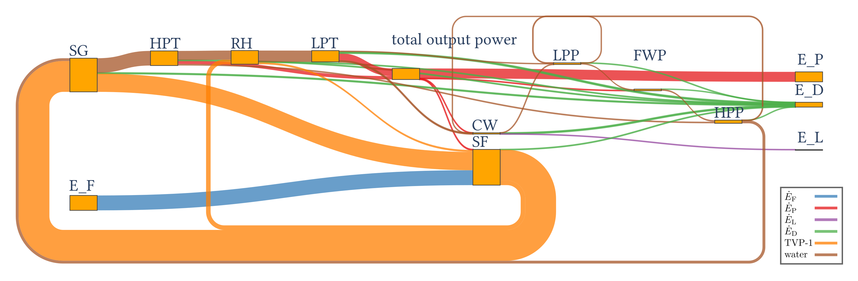
Figure 1. Exergy balance of an open system.
Energies 15 04087 g001
Figure 2. Illustration of use cases for heat exchangers. Not illustrated: variant f.
Energies 15 04087 g002
Figure 3. Simplified structure of the TESPy package and the embedding of the exergy analysis.
Energies 15 04087 g003
Figure 4. Simplified flowchart of the exergy analysis in TESPy.
Energies 15 04087 g004
Figure 5. Flow chart of SEGS implemented in TESPy.
Energies 15 04087 g005
Figure 6. Machine-generated Grassmann diagram based on functional groups of SEGS. The value of the exergy flows are shown in a true-to-scale manner by the width of the edges.
Energies 15 04087 g006
Figure 7. Flow chart of sCO2 power cycle implemented in TESPy.
Energies 15 04087 g007
Figure 8. Machine-generated Grassmann diagram based on functional groups of sCO2 power cycle. The value of the exergy flows are shown in a true-to-scale manner by the width of the edges.
Energies 15 04087 g008
Figure 9. Flow chart of the air refrigeration cycle implemented in TESPy.
Energies 15 04087 g009
Figure 10. Machine-generated Grassmann diagram for the refrigeration cycle. The value of the exergy flows are shown in a true-to-scale manner by the width of the edges.
Energies 15 04087 g010
Table 3. SEGS—Results of the exergy analysis, overall process. All values given in MW .
E ˙ F , tot E ˙ P , tot E ˙ D , tot E ˙ L , tot
47.6331.7715.370.49
Table 4. SEGS—Results of the exergy analysis, functional groups. If not given, dimension of data is MW.
Functional Group G E ˙ in , G E ˙ out , G E ˙ D , G y D , G (%) y D , G * (%)
Low-pressure turbine (LPT)36.0131.944.078.626.5
Cooling water system (CW)4.090.593.507.322.8
Steam generator (SG)107.46104.942.525.316.4
High-pressure turbine (HPT)46.6645.061.603.410.4
Reheater (RH)43.6442.411.232.68.0
Solar field (SF)114.09112.891.202.57.8
Low-pressure preheater (LPP)5.254.510.741.64.8
High-pressure preheater (HPP)10.139.790.330.72.2
Feedwater pump (FWP)5.265.070.180.41.2
Table 5. sCO2 power cycle—Parameters of the overall process and components [75].
ParameterSymbolUnitValue
Turbine inlet temperature T 5 C 600
Turbine inlet pressure p 5 bar 250
Compressor inlet pressures p 1 , p 10 bar 75, 75
Compressors, efficiencies η is , η el , m %85.0, 95.1
Turbine, efficiencies η is , η el , m %90.0, 98.0
Recuperators, lower temperature difference Δ T t , l K 5
Table 6. sCO2 power cycle—Results of the exergy analysis, overall process. All values given in MW .
E ˙ F , tot E ˙ P , tot E ˙ D , tot E ˙ L , tot
154.93100.0054.930.00
Table 7. sCO2 power cycle—Results of the exergy analysis, components. If not given, dimension of data is MW.
Component k E ˙ F , k E ˙ P , k E ˙ D , k ε k (%) y D , k (%) y D , k * (%)
Compressor 147.4940.207.2984.64.713.3
Compressor 237.5832.814.7687.33.18.7
Heater154.93154.090.8499.50.51.5
Recuperator 173.8169.933.8794.82.57.1
Recuperator 2139.19135.433.7697.32.46.8
Turbine197.19185.0712.1293.97.822.1
Water cooler22.28nan22.28nan14.440.6
Table 8. Air refrigeration cycle—Parameters of the overall process and components [76].
ParameterSymbolUnitValue
Compressor inlet temperature T 1 C −30
Compressor inlet pressure p 1 bar 1
Turbine inlet temperature T 3 C 35
Turbine inlet pressure p 3 bar 5
Ambient air temperatures T 21 , T 22 C 25, 40
Refrigeration temperatures T 11 , T 12 C −10, −20
Compressor/turbine efficiencies η is , η el , m %80.0, 96.2
Table 9. Air refrigeration cycle—Results of the exergy analysis, overall process. All values given in kW .
E ˙ F , tot E ˙ P , tot E ˙ D , tot E ˙ L , tot
439.8015.51412.2212.07
Table 10. Air refrigeration cycle—Results of the exergy analysis, components. If not given, dimension of data is kW.
Component k E ˙ F , k E ˙ P , k E ˙ D , k ε k (%) y D , k (%) y D , k * (%)
Compressor815.29674.08141.2182.732.134.3
Cooling heat exchanger46.3015.5130.7933.57.07.5
Heat sink heat exchanger107.3112.0795.2411.221.723.1
Turbine549.60404.62144.9873.633.035.2
Publisher’s Note: MDPI stays neutral with regard to jurisdictional claims in published maps and institutional affiliations.

