Article

Numerical Assessment of a Tension-Leg Platform Wind Turbine in Intermediate Water Using the Smoothed Particle Hydrodynamics Method

by
Bonaventura Tagliafierro
1,
Madjid Karimirad
2,*,
Iván Martínez-Estévez
3,
José M. Domínguez
3,
Giacomo Viccione
4 and
Alejandro J. C. Crespo
3
1
Department of Civil Engineering, University of Salerno, 84084 Fisciano, Italy
2
School of Natural and Built Environment, Queen’s University Belfast, Belfast BT9 5AG, UK
3
EPhysLab, CIM-Uvigo, Universidade de Vigo, 32004 Ourense, Spain
4
Environmental and Maritime Hydraulics Laboratory (LIDAM), University of Salerno, Via Giovanni Paolo II, 132, 84084 Fisciano, Italy
*
Author to whom correspondence should be addressed.
Energies 2022, 15(11), 3993; https://doi.org/10.3390/en15113993
Submission received: 30 April 2022 / Revised: 23 May 2022 / Accepted: 26 May 2022 / Published: 28 May 2022

Abstract

:
The open-source code DualSPHysics, based on the Smoothed Particle Hydrodynamics method for solving fluid mechanics problems, defines a complete numerical environment for simulating the interaction of floating structures with ocean waves, and includes external libraries to simulate kinematic- and dynamic-type restrictions. In this work, a full validation of the SPH framework using experimental data available for an experimental test campaign on a 1:37-scale floating offshore wind turbine tension-leg platform (TLP) is presented. The first set of validation cases includes a surge decay test, to assess the quality of the fluid–solid interaction, and regular wave tests, which stimulate the mooring system to a large extent. During this phase, tendons (tension legs) that are simulated by MoorDyn + are validated. Spectral comparison shows that the model is able to capture the surge and pitch dynamic amplification that occurs around the resonant fundamental mode of vibration. This work concludes with a numerical investigation that estimates the response of TLP under extreme events defined using multiple realizations of irregular sea states; the results suggest that the tendon loads are sensitive to the sea-state realization, providing maximum tendon peak forces in a range of ±10% about the mean. Furthermore, it is shown that the load pattern that forms from considering the relative position of the tendons to the incident wave direction leads to higher forces (≈20%).

1. Introduction

Floating offshore wind turbines (FOWTs) can be used to widen the viable area for wind energy exploitation, allowing turbines to generate electricity in water depths where direct foundations are not feasible and to access locations with higher and steadier wind characteristics. Installing wind turbines offshore is becoming more and more attractive for investors, as larger areas and better wind resources are available [1]. However, to unlock the potential of offshore wind, floating platforms for wind turbines or other forms of connection must be used [2], as bottom-fixed foundations are inadequate.
Different schematics of FOWT foundation technologies are available [3,4]; tension-leg platforms (TLPs), which can provide a sure foot for the installation of wind turbines, gain stability through water displacement and mooring lines. They are based on the TLP system, a preferred solution in the offshore oil sector and their performance is well known; they mainly use vertical tendons to constrain motion along the vertical axis, and can also provide surge constraints at the cost of certain lateral displacements [5]. Moreover, in view of the fact that many devices work together (farms), secondary mooring systems can be used to keep the station horizontal and provide redundancy to the overall system [6]. As a fully complementary concept, for the spar-type floating wind turbine (SFWT), there is no noticeable transition from tower to float (spar), and the design and construction of the floating tower should be carried out seamlessly. Different mooring line systems can be used for stability purposes, using either catenary or tendon, or a combination of both [2,7].
Due to the fact that these structures are in their early prototype development stage, numerical tools can be very useful for investigating their response [8]. Accurate simulation of the fluid mechanics requires the use of Computational Fluid Dynamics (CFD) methods, but it is also important to pay attention to simulating the multiphysics nature of these systems [9,10]. Offshore wind turbines entail novel challenges for the overall aerodynamics due to the multiphysics nature of the system [11], and a large part of the existing literature has not considered the coupling between the wave- and wind-induced motions yet [12], which has been proved relevant by the main conclusions reached during the Offshore Code Comparison Collaboration Continuation, with Correlation project (OC5) [13]. High-fidelity modeling procedures to solve the dynamics of the system are indeed necessary to obtain reliable model results [14]. It is interesting to mention that, although the main focus of certain research projects, such as the OC6 (Offshore Code Comparison, Collaboration, Continued, with Correlation and unCertainty), is on the validation of engineering-design tools for offshore wind turbines, the latest testing campaign outcome of Phase Ib [15] has a broader scope and is suitable for CFD code validation.
Modeling marine structures in extreme wave conditions is difficult and costly, both experimentally and numerically. To a certain degree, some investigations can be carried out experimentally, but for real-scale models and coupling between wind, current, and wave actions numerical simulations seem to be the only way forward. For handling simulations of energy capturing devices at sea, CFD methods are the best option [16] since, in principle, they could be used to simulate fluids in detail. Much progress has been made in recent years, but classical mesh-based CFD methods still tend to fail in very harsh wave conditions [17]. Nevertheless, successful applications of mesh-based CFD solvers in solving the hydrodynamics of marine structures for renewable energy have shown that they can provide a high degree of accuracy [18,19,20].
An environment that has been revealed to be suitable for such usages, especially within engineering fields of application, is the one established by meshless methods [21,22,23,24,25]. The Smoothed Particle Hydrodynamics (SPH) method employs a set of a finite number of discrete particles to represent the state of a system and to record its movement [26]. Each particle is generated to represent a part of the continuum problem domain. For CFD problems, each particle has a set of field variables, e.g., mass, momentum, energy, positions, and other variables (vorticity, etc.) related to the specific problem. The contribution of those particles is weighted using a kernel function, with an area of influence that is defined using a characteristic smoothing length.
The open-source code DualSPHysics [27] is an advanced meshless solver with emphasis on free-surface flow modeling, based on the SPH technique. Throughout many published research reports, a few of which are reviewed in Luo et al. [25], it has shown outstanding features in supporting simulation of coastal and ocean structures. The coupling with other open-source computing libraries, e.g., Project Chrono [28], or MoorDyn [29], has introduced many versatile features conveniently deployed to simulate multiphysics systems. A large body of research shows that the code can be used for research investigations of marine vessels [30,31,32,33] and also of wave energy converters (WECs) [34] such as: oscillating water columns [35,36]; an oscillating wave surge converter [37]; and point-absorber devices [38,39,40,41,42]. Recent research papers have proposed methods to include flexible elements, such as beams, within the same SPH framework [43,44] that may open up new modeling strategies for devices for renewable energy.
Up until now, there have been flourishing research activities on the development of software that is usually designated as engineering tools. Apart from analytical models [45], the latter identifies numerical tools that are able to perform time domain simulations of marine structures and several environmental conditions. Developed by researchers from the National Renewable Energy Laboratory (NREL), FAST (Fatigue, Aerodynamics, Structures, and Turbulence) [46] is one of the most used open-source codes for marine structures for which wind-, wave-, and current-induced loads provide critical contributions to the overall system response. FAST, however, solves the hydrodynamics with a potential-flow solver (HydroDyn), which is generally unable to capture viscous effects and wave breaking, for example; most of its limitations are worked around by including fictitious treatments for the viscosity and other effects. Tran et al. [47] demonstrated that by comparing the prediction of FAST and a CFD-based solver, potential-flow based models show consistent over estimation when the motion of the investigated platform increases [5,48,49]. Other similar comprehensive research is presented in Liu et al. [50], where an open-source CFD-based solver is used to investigate the performance of the DeepCWind semi-submersible floating wind turbine within a realistic environment, including waves and winds within the same setup. Although combined design strategies (see, e.g., for similar applications, [51,52]) still yield the best performace/cost ratio, the work [50] suggests that the use of CFD can be of great help for the development of offshore technologies, identifying the need for new research. Specifically, one of the gaps brought to light was the lack of accuracy (under prediction) for the mooring line loads, due to the use of a static model to simulate the connections.
The objective of this work is to establish and validate an initial setup for a tension-leg platform for FOWTs with the meshless DualSPHysics code, validating for the first time tendon lines simulated by the MoorDyn + library. Particularly relevant is the validation of the predicted mooring stress driven by the regular wave-induced motion that resolves in high platform displacement. A reference geometry concept investigated in [5] is used to build the numerical model; the experimental data is afterward used to compare and to assess the level of accuracy that can be achieved by performing CFD simulations within the Lagrangian SPH framework. The validated model is then used to investigate the effects on the anchoring systems of extreme wave conditions using irregular sea states. The paper is arranged as follows: Section 2 provides the mathematical description of the SPH method and gives some details on the software implementation; Section 3 presents the experimental setup along with the test matrix that is used for the TLP motion validation, immediately followed by the numerical model definition. In Section 4, the various response amplitude operators are defined and compared to the reference ones. In Section 5, the numerical investigation of the TLP wind turbine under irregular sea states is performed, paying attention to the effects of the sea-state realizations on the mooring line load trends; Section 6 closes this work with a discussion of the prediction capabilities of the presented model and the possibility for future applications.

2. The SPH Method

2.1. Fundamentals

Using the SPH method, a generic function, F, can be defined by:
F ( r ) = F ( r ) W ( r r ) d r
where r is the position vector of the calculation point, r is the position vector of another computational point, and W is the kernel function [53]. The function can be approximated by performing the particles’ contribution within the compact support of the kernel:
F ( r a ) b F ( r b ) W ( r a r b , h ) m b ρ b
where subscript a indicates the interpolated particle, b is a neighboring particle, m and ρ are, respectively, the particle mass and the density, m b / ρ b is the volume associated with the particle b, and h is the smoothing length. The kernel function W is defined in such a way that the positivity on the compact support, normalization, and monotonic behavior are guaranteed [54]. The version of the code employed in this work makes use of the so-called piecewise polynomial Quintic Wendland weighting function (QW) kernel, as defined in [55] and reported here:
W ( q ) = α D 1 q 2 4 ( 2 q + 1 ) 0 q 2
where α D is the scalar that ensures kernel normalization, q = r / h is the non-dimensional distance between particles, and r is the distance between particles a and b.

2.2. Governing Equations

The SPH method is used to represent fluid volumes by defining sets of particles on which the Navier–Stokes (N-S) equations are solved. Within a Lagrangian framework, the differential form of the NS equations is written using the SPH formalism as follows:
d v a d t = b m b p a + p b ρ a ρ b a W a b + g + b m b 4 ν 0 r a b · a W a b ( ρ a + ρ b ) ( r a b 2 + h 2 100 ) v a b
d ρ a d t = ρ a b m b ρ b v a b a W a b + 2 δ h c b ( ρ b ρ a ) v a b a W a b r a b 2 m b ρ b
where t is the time, v is the velocity, p pressure, g is the gravitational acceleration, a is the gradient operator, W r the kernel function, δ is a parameter that governs the diffusive term, ν 0 is the kinematic viscosity, r a b = r a r b with r a and r b being the position of particles a and b, respectively, and c is the speed of sound.
The last term in the momentum equation (Equation (4)) defines the laminar viscosity model according to the formulation proposed in Lo and Shao [56]; the fluid is numerically identified by its kinematic viscosity herein set to 12 6 m 2 /s (water 15 C). As mentioned before, the continuity equation (Equation (5)) comprises a term that is arranged in order to filter high-frequency numerical noise out, which improves the stability of the scheme. Its formulation, as introduced in [57] and further developed under the name of delta-SPH in [58]; it is based on a density diffusion term, which affects the density field, providing more physical agreement when mild density variations are in place. Furthermore, this second term makes use of the formulation proposed in Fourtakas et al. [59,60] by considering the dynamic component of the density field to control the intensity of the diffusive term.
A weakly compressible SPH formulation (WCSPH) is used here for modeling Newtonian fluids, following Tait’s equation of state to determine the fluid pressure, p, from the density field, which is given by:
p = c 2 ρ 0 γ ρ ρ 0 γ 1 ,
where ρ 0 is the reference fluid density ( 998.5 kg/m 3 for fresh water), γ is the polytropic constant (set to 7 for water-like fluids). Within a WC formulation, the fluid compressibility can be adjusted to ensure reasonable values for the integration timesteps and without losing precision for the pressure field.

2.3. Rigid Body Dynamics

DualSPHysics implements the equations of rigid body dynamics to compute the motion of rigid instances interacting with fluid particles. Each boundary particle that composes the rigid object, k, experiences a force per unit mass given by:
f k = g + b f l u i d f k b
where f k b is the force contribution of the fluid particle b, per unit mass, on the boundary particle k. The basic equations that are used for the motion of rigid bodies are:
M d v d t = k b o d y m k f k
I d Ω d t = k b o d y m k ( r k r 0 ) × f k
where M is the matrix mass of the object, I is the matrix of the moment of inertia, v is the velocity, Ω is the angular velocity, and r 0 is the center of mass; × indicates the cross product. Equations (8) and (9) are integrated in time to evaluate the values of v and Ω for the next time step. The boundary particles receive a velocity according to:
v k = v + Ω × ( r k r 0 )
The final step of each solving model loop rearranges the boundary particles according to the integration of Equation (10) in time. In the literature, some research has shown that this approach preserves the linear and angular momentum [61], and other research has provided validations about buoyancy-driven [62,63] and fluid-driven motion [64].

2.4. Adopted Boundary Conditions

Crespo et al. [65] presented the Dynamic Boundary Condition (DBC) which was implemented as a standard method for the definition of the boundary conditions in DualSPHysics. The DBC treatment has been demonstrated to work properly in many applicative cases [66]. In the wake of minor inconsistencies in the DBC approach, such as large gaps appearing when transition from non-wet to wet takes place, a novel formulation was proposed in [67]. The so-called mDBC (modified DBC) works with the same particle arrangement defined for its former version, but it uses a boundary surface to locate the layer transition between the body and the fluid domain. The surface is used to mirror ghost nodes from the boundary particles into the fluid domain and hence evaluate the fluid properties at these virtual positions; the SPH computation thus exploits the values mirrored on the boundary particles to approximate the fluid particle interaction [68]. The use of mDBC guarantees precise pressure computation, as shown in [67,69], and reduces the non-physical gap between boundary and fluid particles, which is very useful for simulations of engineering problems [70,71].

2.5. Coupling to MoorDyn +

For the case under study, the correct simulation of the mooring lines is vital, as wired connections are often exploited in offshore structures for their capacity to provide connections spanning long distances with a small usage of material. The correct estimation of the tendon performance is critical to the understanding of anchored floating structures, and DualSPHysics does indeed allow one to perform multiphysics simulations by using coupling strategies between different pieces of software, managing different differential systems of equation solvers (some examples are in [62,72,73]). In this way, a fully Lagrangian 3D environment that contains the geometry for the whole system is created, and here the effects of mooring lines on floating structures are addressed by the MoorDyn + library [74].
MoorDyn + solves the mooring dynamics using the lumped-mass approach inherited from its parent version MoorDyn [29]. This version of the code has seen several improvements, such as solving interconnectivity among floating bodies and using different bottom depths for catenary-like connections. The library computes the tension at the anchor and fairlead points that are then used to evaluate the final motion of the structure following Equations (8) and (9). As such, the formulation is generally suitable for simulating any kind of cabled connection; tendons have not been validated yet. The two-way coupling structure presented in [63] is used for the data exchange between the DualSPHysics main loop and the MoorDyn + .
When the lumped-mass approach is used for simulating structural elements only reacting to tension forces, single mooring lines (of initial unstretched length l 0 ) are arranged into equally spaced N + 1 nodes, connected by N equally long segments. Each segment inherits its properties from the overall geometry of the line, given as: segment length l = l 0 / N ; volume-equivalent area A = π / 4 d 2 , with d being the volume-equivalent diameter; density ρ m ; net mass m i = A l ( ρ m ρ w ) , with ρ w being the water density. The boundary conditions are set at both the fairleads and the fixed connections, which represent the interfaces over which the MoorDyn + library and the DualSPHysics code communicate.

3. Numerical Modeling

3.1. Experimental Setup

The study involved a 1:37 geometric scale model (Froude similarity) of a TLP, which houses a stiff rod that represents an idealized wind turbine tower; it was tested in the Kelvin Hydrodynamics Laboratory at the University of Strathclyde (UK) under regular and irregular waves (Figure 1); the experimental and numerical campaign is presented in Oguz et al. [5]. The superstructure configuration closely represents the NREL 5-MW baseline wind turbine [75]. Geometrically speaking, the reported data in [5] can be used to rebuild a quasi-similar setup, with enough information to perform a complete validation by contrasting against the motion response amplitude operators (RAOs) for the platform’s surge and pitch modes. Furthermore, the dimensionless response spectra for the mooring tension can provide a reference dataset for the definition of tendon tension transfer functions.
The reference paper explores the capability of the open-source solver FAST (Fatigue, Aerodynamics, Structures, and Turbulence) [46], developed by researchers from the National Renewable Energy Laboratory (NREL), to simulate the same TLP configuration under scenarios including wind forces. First, the numerical setup in the above-mentioned numerical study is used to provide another reference solution to compare with. For the scope of this work, regular wave conditions will be defined in the following and used to build the numerical RAO for the surge and pitch motion and the tendon tension transfer functions for two mooring lines, namely, T 1 (bow) and T 5 (aft), as indicated in Figure 2.

3.2. Numerical Model

The model building process and the validation procedures are presented at model scale, meaning that the geometry is reproduced at a 1 to −1 ratio, thus making direct comparison to the experimental results. Two spatial discretizations of the numerical model, usually indicated by the initial interparticle distance ( d p ), are set. According to the smoothing length, h, which is given as h = 1.20 3 d p within the scope of this paper, a minimum number of particles is indeed necessary to assure the correct use of mDBC so that during the fluid–solid particle interaction [67], the kernel comprises enough particle contributions to compute the field variables with sufficient accuracy. SPH-L = 0.03 m (low) and SPH-H = 0.02 m (high) are defined such that they guarantee five and seven particles, respectively, in the reference dimension, that is, the pontoon width, 0.120 m.

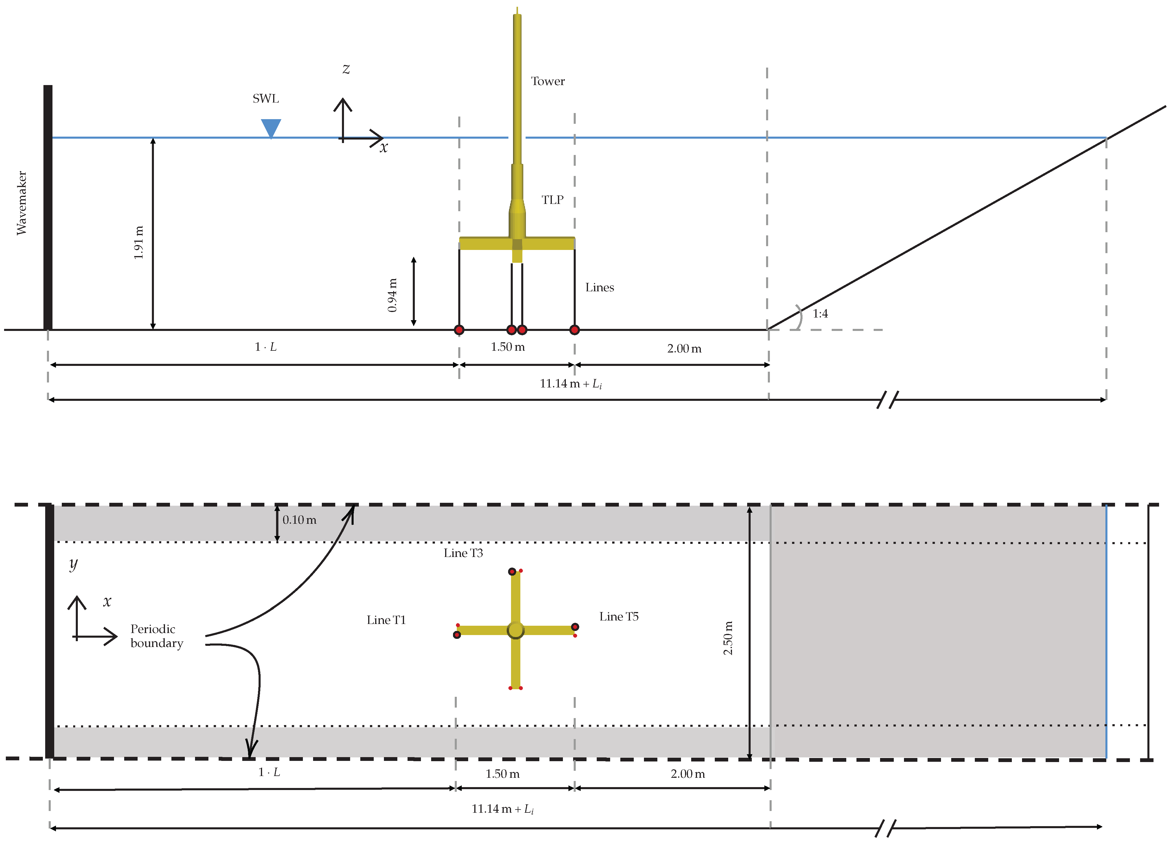
3.2.1. Wave Tank Design

A basin of 76 × 4.6 m, 1.90 m water depth was used for the experimental tests. Figure 2 proposes a revisitation of the wave tank through its novel design, for which the lateral and top views are sketched. The tank used for this investigation was reduced in length and width in an attempt to mediate accuracy and computational runtime, whereas the depth is preserved to avoid introducing wave profile disturbances. The tank is shortened owing to a piston-type wavemaker equipped with an active wave absorption system (AWAS), following the implementation proposed in [76], to guarantee the correct input incident wave. Note that the flume length, defined as L i in Figure 2, indicates the wave length of the wave being generated, and is computed by solving the dispersion formula:
ω i 2 = g k i tanh ( k i · d )
where g is the magnitude of the gravity acceleration vector, k i = 2 π / L i is the wavenumber, ω i = 2 π / T i is the angular frequency with T i being the wave period, and d is the water depth. To prevent lateral reflection, since the tank does not cover the experimental full width, the width is set to twice the apparent diameter of the floater in conjunction with numerical damping zones at the lateral edges (gray shaded area in the top view in Figure 2); lateral solid walls are replaced with periodic boundary conditions [77].

3.2.2. Mooring Systems

The eight tendons (highlighted in Figure 2) that are used to provide anchoring to the TLP configuration are modeled using the mooring systems available in the MoorDyn + solver. When the lumped-mass approach is used to model cables, it usually introduces higher modes of vibration along the axis of the line, which may provoke nonphysical node oscillations, which tendons are extremely sensitive to. The formulation presented in [29] works around this issue by introducing a viscous damping term that can smooth down the vibration modes with frequencies close to the critical one. The natural frequency can be defined as:
f n = 1 π l E ρ .
where l is the length of each line segment and E is the elasticity modulus of the line.
The input data used in the numerical model are reported in Table 1. The initial (unstretched) length of the eight tendons is l 0 = 0.940 m, as is shown in the geometrical setup in Figure 2, and the nominal diameter is d = 4.00 mm. To proceed with the parameter assignment, the mechanical properties of the tendon material (nylon) are used to identify the stiffness of the cross section. The presence of an in-series spring for each tendon in the experimental setup, in this work, is accounted for by considering an over-relaxed value, specifically one third of the initial cross-sectional stiffness. Note that the model time step ( d t M ), the internal integration time-step used in MoorDyn + , is defined according to the following relationship d t M = 20 f n , whereas N = 20 segments are used for there is no expected slackness for the investigated set of wave conditions. MoorDyn + solves the 3 ( N + 1 ) equations of the motion using a constant-time-step second-order Runge–Kutta integrator.

4. Validation

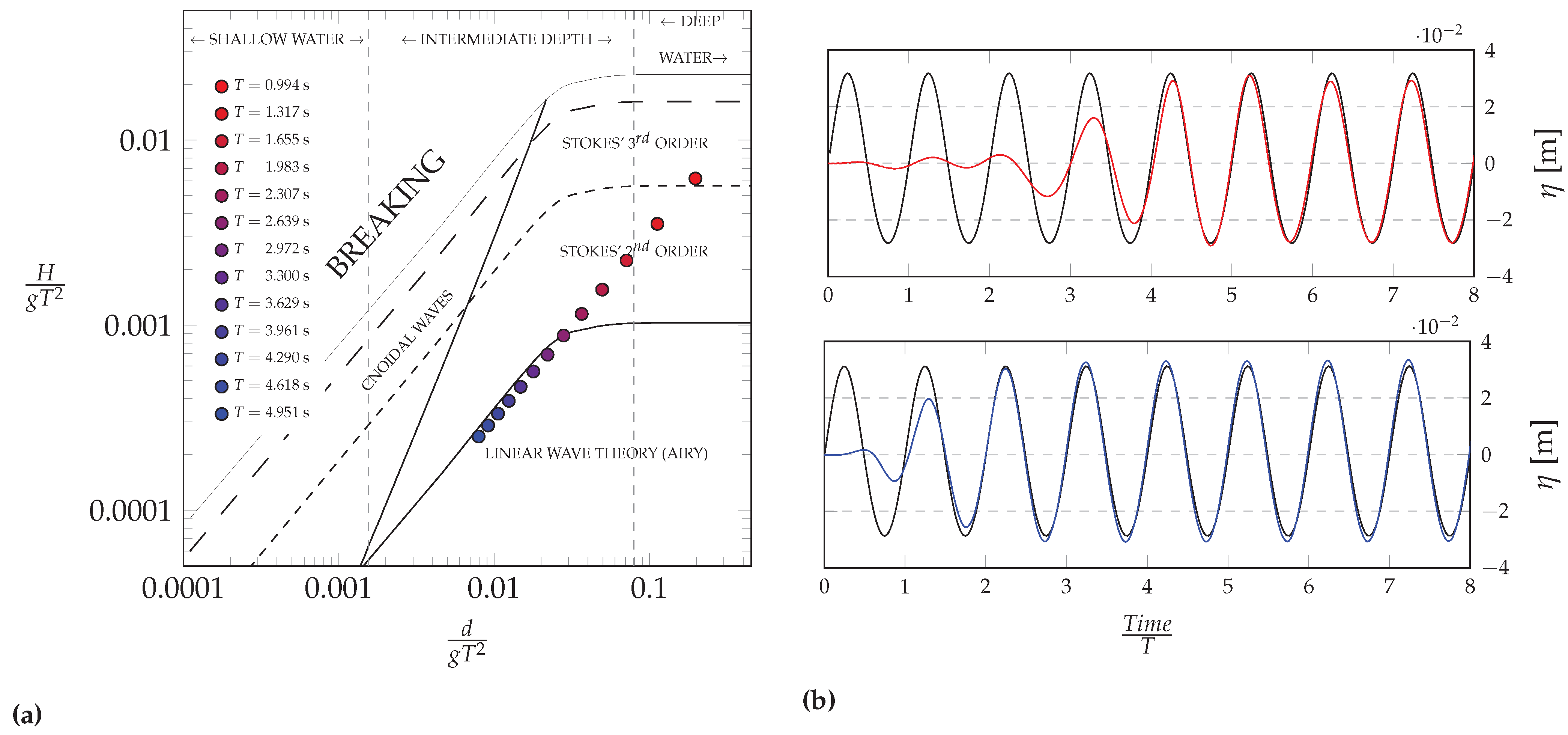
4.1. Wave Generation and Propagation

First of all, Figure 3a charts the wave conditions that are used for the definition of the validation test matrix, following the same procedure proposed in the reference paper to build the surge and pitch RAOs and the tension transfer functions. A preliminary study of this setup is presented in [78].
The Le Méhauté’s abacus [79], presented in Figure 3a, classifies the regular wave conditions according to the theoretical model that should be used for their generation theory and the steepness–shallowness ratio. All the considered regular waves can be safely simulated by employing second-order Stokes’ theory. Case T = 0.994 s, being the only outlier, is positioned relatively close to the Stokes’ second order area, thus producing little to no third-order term magnitude of the Stokes’ perturbative series with respect to the second order terms. Note that Le Méhauté’s classification places the waves in a straight line since they all share the same wave height 0.060 m and propagate in the same water depth 1.91 m.
The wave tank capability in generating and propagating waves is ascertained using the two limit cases of the range for the wave conditions, Figure 3a. The waves correspond to T = 0.994 and T = 4.951 s and both have the wave height H = 0.060 m, and propagate in 1.91 m water depth (deep water and intermediate depth, respectively). A visual comparison of the wave generation and propagation performance of the set wave tank is given in Figure 3b, which charts the free-surface elevation at the float’s location against the expected theoretical second Stokes’ theory wave profile; the model delivers good agreement in both wave amplitude and overall shape. The anti-reflective beach downstream from the propagation domain provides a reflection coefficient lower than 2%, as computed using Healy’s method [80].
A final note on the computational performance of the model, according to the two resolutions, seems to be appropriate. As the definition of the tank length is parametric, a case representative of the batch of simulations is considered to showcase the features of the model and its computational cost. In particular, Case T = 3.300 s, with wave length corresponding to L = 12.60 m, yields to 3.42 and 5.80 M particles, respectively, for SPH-L = 0.03 m (low) and SPH-H = 0.02 m (high). The simulated physical time is 14 × T , so 54.5 s, and runs in 36 and 79 h, respectively, on a NVidia Tesla V100-SXM2-16GB (CirrusII HPC system).

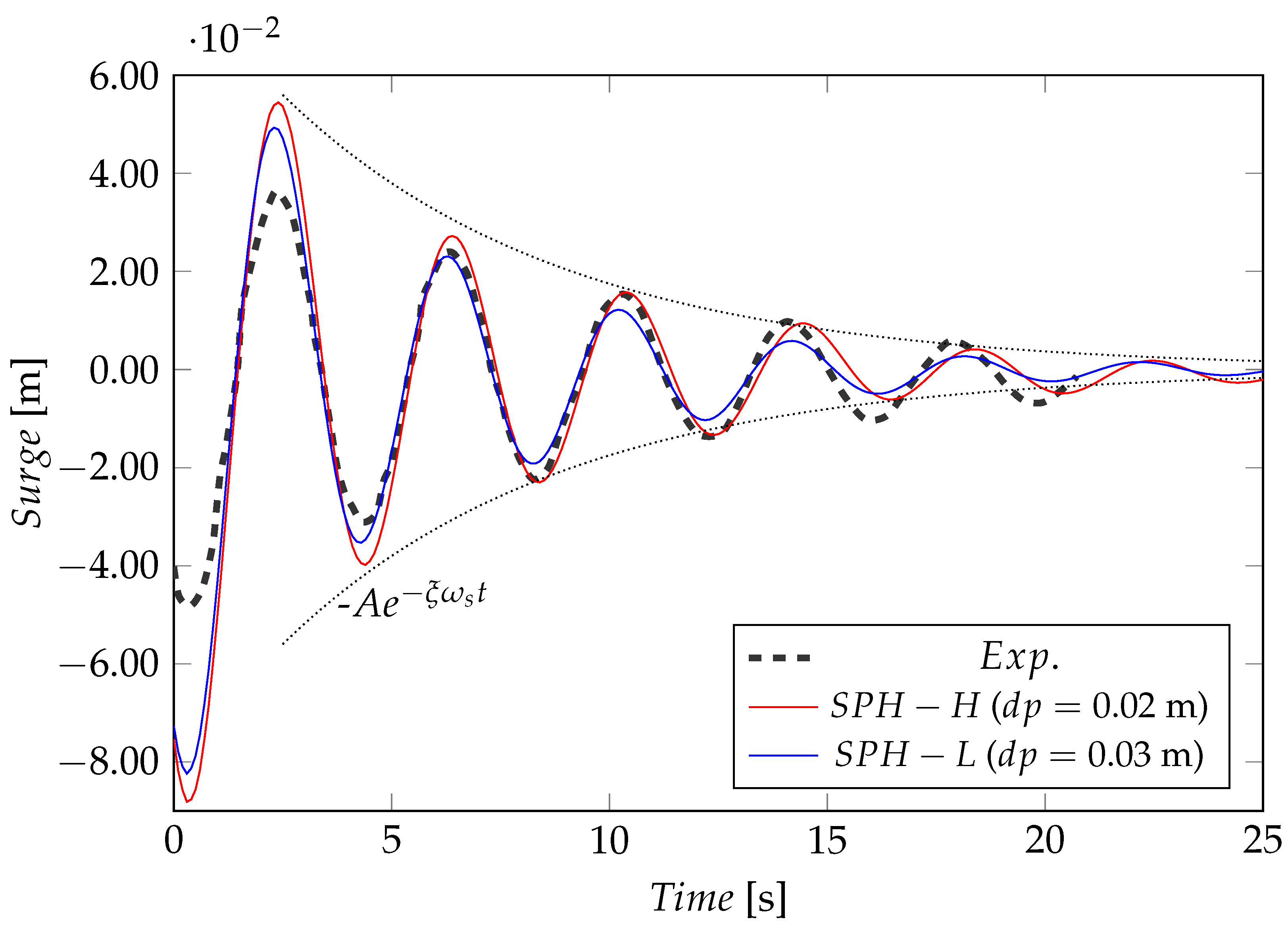
4.2. Surge Decay Test

The preliminary study of the revealed TLP presented in [78] suggests using the following data to initialize the TLP mechanical properties: mass, consistent with a period T s . e x p = 4.05 s ( 24.38 s at full-scale), of 47.74 kg, and an inertia matrix defined as diag( I x x = I y y = 126 , I z z = 5 ) kg·m 2 . The solid geometry of the TLP has been used to distribute the mass evenly across the surfaces that compose the outer shape of the body. A decay surge decay test is still performed to validate the initial setup.
The test is performed in a 3 × 3 m tank, shown in Figure 4, brimmed with damping areas to avoid water surface disturbance being re-reflected; an initial surge displacement (≈0.08 m) was imposed on the structure, and then left free to oscillate under the recentering effect provided by the tendon system. The time evolution of the TLP surge motion for the decay test is shown in Figure 5. In order to estimate the natural period of the structure T s , the solution for the equation of motion is considered. The transient term preserves its exponential form when written in terms of displacement, yielding to A ( ξ ω s t ) , where A is the initial signal amplitude, ξ is the damping ratio, ω s is the circular frequency of vibration of the system, t is the time. Two curves, coming from the above transient term, are introduced upon the surge free vibration evolution. The best fit is given by A = 0.060 m, T s = 4.02 s, and ξ = 0.10 . The period was double-checked with a spectral analysis based on Fourier Transform, which confirmed the obtained value. The period T s . n u m = 4.02 s (vs. T s . e x p = 4.05 s) is achieved, and shows an error of 0.90 % with respect to the experimental one.

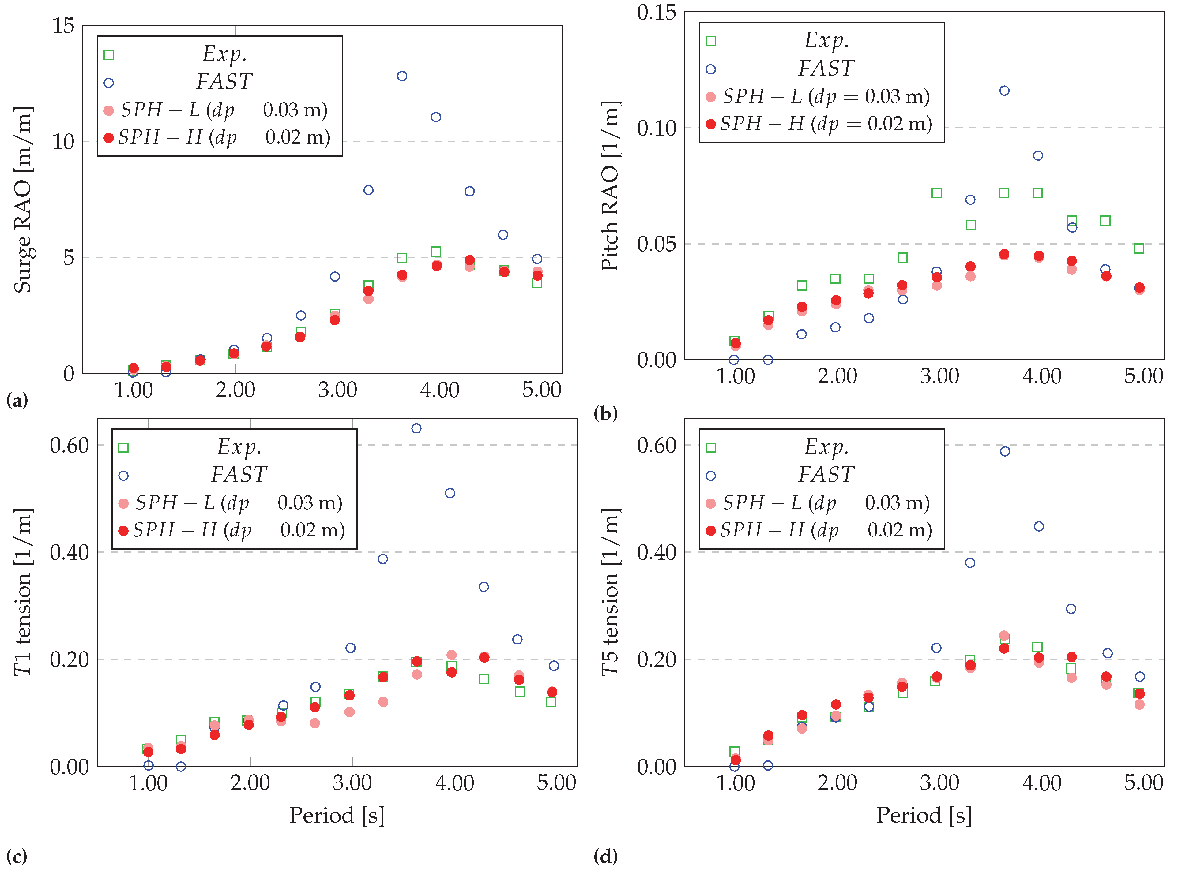
4.3. Surge and Pitch Motion Spectra

The final validation of the numerical model is performed by considering a spectral reconstruction of the surge and pitch motion spectra, which are therefore compared to the data available in reference work, Oguz et al. [5]. A rich spectrum of components that cover from 1.00 to 5.00 s is considered to build the system response; the corresponding waves are classified in Figure 3a. It is worth mentioning that the considered frequency range contains the fundamental period of vibration for the surge mode, previously defined.
Figure 6 resumes the results of the numerical campaign performed on the TLP under the regular wave conditions defined in Figure 3a. The four charts compare the surge and pitch response predicted by the presented model (SPH) to the experimental data (Exp.) and to the results of a FAST numerical model (FAST). The surge and the pitch motion, and the T 1 and T 5 tension values are calculated by averaging values of the peak response over a time window that covers six wave periods. That time window was preceded by four wave periods which proved necessary in order to obtain a steady and fully developed system response. The response amplitude operators are defined by using the wave height gauged for each case; the dimensionless tendon tension F ¯ is evaluated as:
F ¯ = F F s t i l l F s t i l l
where F is the tension estimated from the simulation and F s t i l l is tension induced by the extra platform buoyancy.
The comparison in Figure 6a demonstrates that the proposed numerical setup is able to correctly predict the system’s response within the considered spectrum of frequencies. The agreement is almost perfect for the examined wave conditions, and the surge displacement peaks exactly around the expected period (≈4 s). The pitch response Figure 6b spectrum shows good agreement as well, with an almost insignificant disagreement that is likely due to having considered stiffer tendons than they were in reality. Nevertheless, the pitch angle underestimation, for some cases, does not substantially affect the quality of the surge motion model prediction because this phenomenon only takes place thanks to the tendons’ deformability and thus it does not affect the overall hydrodynamics response of the TLP. It is important to mention that, throughout the whole numerical investigation, the tendons never experienced loss of tension. The tension force transfer functions depicted in Figure 6c,d provide very good estimation of the anchoring system peak response and they shape trends close to the experimental ones. The numerical investigation for which the data are reported here can be likened to the validation proposed in [81], in which the dynamic properties of a semi-submersible platform are validated using a regular wave spectrum. Similar accuracy is shown for the motion of the platform but the paper [81], does not include any prediction of the mooring line tensions.
The charts in Figure 6 suggest that the SPH model used here to solve fluid mechanics can capture the relevant characteristics of the interaction between waves and structures. Noteworthy is the accuracy of the proposed model in predicting the response of the system for the most nonlinear cases, that is, the smallest frequencies. As discussed in the introduction to this paper, the fluid solver used in the FAST framework, HydroDyn, is unable to provide sufficient excitation force to the rigid TLP system. By considering the authors’ comments in [5]—“The free oscillation test data were analyzed to give linear and quadratic damping for the platform. In principle this data might have been used to improve the correlation between numerical results and experimental predictions. However, the version of FAST used for this study did not allow additional viscous hydrodynamic damping […]” (reprinted from Oguz et al., [5] copyright (2022), LN 5311960964922, with permission from Elsevier)—it is possible to conclude that viscous forces are accurately reproduced when a laminar viscosity treatment is introduced within the SPH formulation. The FAST model that was used for the reference numerical study, which overestimates the TLP motion almost twofold around resonant frequencies, did not consider additional viscous damping parameters, as shown in [82].
Before starting the numerical investigation campaign, another test is proposed to evaluate the accuracy of the fluid force estimation when passing from a very refined condition (i.e., SPH-H) to a coarse one (i.e., SPH-L). Figure 7 provides the maximum fluid forces (heave and surge) on the TLP for the regular waves considered in the previous validation. The trends in the plot reveal that the fluid forces are consistently estimated for the two resolutions over the entire spectrum. This gives the option to use the least expensive resolution SPH-L for the next investigation. Viscous effects have been considered to be of vital importance for the estimation of loads, especially for extreme conditions. The research proposed in [83] shows the relevance of this effect for the hydrodynamic response of FOWT when a WEC is also included in the same setup.

5. Numerical Investigation

This section provides the dynamic response of the TLP wind turbine under two irregular sea states, and for each one, four different stochastic realizations for the phase components are created in order to define four free-surface profiles that differ for peak position but comply with the target spectrum.

5.1. Irregular Sea States

According to the independent organization DNV (Det Norske Veritas), for structures with significant dynamics response, stochastic models should be used to describe the free surface and its kinematics [84]. For similar representations, it is necessary to use the definition of the time evolution of the sea state, mostly characterized by the environmental parameters: significant wave height ( H m 0 ), and a wave frequency spectrum ( S ω ); both define two constraints for the definition of the the surface profile evolution. Usually, these two mentioned parameters identify a storm event in a given area according to an arbitrarily defined event return period. One of the most recognized approaches for shaping S ω is based on a Joint North Sea Wave Observation Project (JONSWAP) wave power spectrum definition [85], which goes:
S J P ( ω ) = α g 2 ω 5 exp 5 4 ω p ω 4 γ exp ( ω ω p ) 2 2 σ 2 ω p 2 ,
where ω = 2 π / T is the angular frequency, ω p = 2 π / T p is the spectral peak angular frequency, α is the generalized Phillips’ constant, g is the magnitude of the acceleration of gravity, γ is the peak enhancement factor, σ is the spectral width parameter, which is 0.07 for ω p ω and 0.09 for ω p < ω .
For irregular waves, the surface elevation is calculated based on linear wave theory with a second-order correction, including both long-crested waves and super-harmonic components. The ith component of the free surface is given:
η i = A i c o s ( ω i t + ϕ i ) + k i A i 2 3 c i 2 4 c i 3 c o s ( 2 ( ω i t + ϕ i ) ) ,
where A i is the amplitude, k i = 2 π / L i ( L i is computed using (11)) is the wavenumber, c i is the radiant wave frequency, and ϕ i is a term that can include a phase shift. The randomness of the final free surface evolution, which results from composing an adequate number of components, has two degrees of freedom given by the randomness of A i and ϕ i .
The most severe condition tested in the reference paper corresponds to a 100-year return period event in the North Sea; it is considered here and the parameters that define the demand spectrum are given in Table 2, sea state S. Additionally, a slight modification of sea state is considered for the purpose of this investigation for which the peak period is 10% longer (the calculation refers to full-scale figures), and is defined in the second row of Table 2, sea state V. Following the recommendations in [84,86], 1024 wave components are combined to define such long time series (about 1200 × T p ), and such a high number proves necessary to avoid group repetition and thus maximize the free-surface randomness.

5.2. Simulations

The time series of irregular waves in Table 2 are generated from the JONSWAP power density spectrum by means of an automated tool embedded in DualSPHysics [72]. A stretched algorithm as described in [76] is used to define the spectral bandwidth discretization so that many more frequency components are representative of the most energy-rich part of the spectrum. The said internal tool for the time series generation allows for the definition of seed numbers that are used for the generation of the uniform distribution of ϕ i to be plugged into (15).
The numerical tank configuration, which has been presented and validated in Section 4.1, is utilized for the generation and propagation of the irregular wave trains; the distance between the wavemaker and the TLP is set to 6.00 m for both cases in Table 2. The piston motion is computed by an internal routine according to the parameters presented in Table 2, and corrected in time by an AWAS system. With the stated accuracy shown by the model for the validation campaign, the resolution defined as S P H L ( d p = 0.03 m) is used for the initial geometry discretization; it yields almost 2.5 million particles, for which the total elapsed time is reported in the last column of Table 2.
By means of a frequency domain analysis performed using a Fourier Transform analysis, the accuracy of the system in generating and propagating the proposed waves is assessed; the signal plugged into the FT function comes from the wave surface elevation probed at the TLP location (1 m on the left). The reference wave density spectrum (JONSWAP), and the numerical wave density spectra obtained for the four realizations of sea states S1S4 are compared in Figure 8. It shows that the generated surface meets the target free-surface elevation with sufficient accuracy, capturing the peak period with almost no deviation from the target one, with a slight overestimation of H m 0 of about 4% for S2S4. Note that the cut-in tail of the numerical spectra show a slight offset, whereas the cut-out frequencies are well reproduced. Figure 9 depicts the free-surface time evolution for sea state S3 in which the highest wave amplitude occurs. The free surface is compared to the target one (dashed line), from which it can be seen that there is some inconsistency in wave generation, probably due to the presence of some reflection from the TLP bulk that thus triggers the AWAS system, causing minor mismatching in the wave profile. However, it can be noted that the crest–trough amplitude stays the same for most of the wave train. Additionally, Figure 9 reports the platform surge motion evolution as well; it is clear that there is phase lag between the wave peaks and the surge motion of the platform that is mostly caused by the misalignment between the characteristic wave periods and the TLP dynamic properties.
The numerical model outputs for the four realizations of sea states S and V presented in Table 2 are elaborated in accordance with the steps presented in the following. The free-surface evolution probed on the TLP side in each test is spliced into single-period intervals, T i , with an up-zero-crossing algorithm; following the recommendation provided in [84], the zero-cross procedure was set to include in each time window a trough and the ensuing crest; other applicative examples can be found in [42,87]. In agreement with each zero-cross interval T i , the time series for the line force is partitioned and in each T i , the force peak is taken, that is, F i = m a x ( F l i n e ) . Using (13), the data for the forces are made dimensionless, as in the previous validation procedure, to have a more general understanding of the system dynamics evolution.
Figure 10 shows the probability density functions (PDFs) for the dimensionless force peak series corresponding to the four irregular wave tests S1S4 (a) and V1V4 (b). The colored curves in the charts are grouped according to the tendon line they refer to, whereas different line patterns correspond to the sea-state realizations. In general, the distributions of the force when analyzed for each sea state prove to be quite consistent for the different realizations; furthermore, they all are unimodal. Lines T 1 (front tendon) and T 5 (back tendon) have close expected values, with similar modes around 0.35 Δ F / F s t i l l , which, however, see remarkable differences accounting for the sea-state realization. Line T 3 (middle line) experiences a pattern of force that is much more consistent than the external ones, with a distribution being characterized by small dispersion and the data being almost symmetrically distributed with respect to the expected value. Sea states S to V prove to affect the load magnitude similarly, at the least when the expected values of the distributions are considered.
For these two sea states, S and V, the distribution shapes are also charted using exceedance probability functions, which allow more efficient inspection of the extreme values, characterized by a reduced number of occurrences. The dataset for the extreme value analysis shown in Figure 10 provides a substantial estimate of the maximum loads that may occur for the specified event return period. The presence of a consistent deviation between the expected loads for the front and the back tendons is captured by the proposed numerical modeling owing to its capacity to correctly capture the coupling between the fluid and the structure motion. On average, for sea state S, the design load for the front tendons is 0.83 Δ F / F s t i l l , whereas for the back tendons it is 1.02 Δ F / F s t i l l . Concerning sea state V, with its energy content bulk being closer to the surge mode, higher forces are experienced, providing, on average, 0.98 Δ F / F s t i l l for the front tendons, and 1.17 Δ F / F s t i l l for the back tendons.
The use of extreme events for the definition of limit states for FOWT is enforced by practice recommendations, and this research proposes a tool for the estimation of extreme mooring line loads using a validated model. Opposed to the definition of real sea states, as employed in this work, another interesting assessment of the performance of a similar moored structure subject to focused waves, which is another model for extreme events [88], can be found in [49]. Other research on a similar subject is presented in [48,81], which unfortunately was limited to regular wave models.
Finally, the dependence of the exceedance probability on the sea state realization suggests that more than one realization should be tested to obtain more reliable information concerning the process, and that a correct estimate of the maximum forces is indispensable to include non-resolved fields on motion to account for the hydrodynamic interactions, and for the nonlinear components in the wave train. The knowledge gained in similar analyses, even though performed only numerically, can be of great use to ensure the correct design of the pieces of equipment that all together make the energy conversion process possible [4]. For example, it could be used for the estimation of mooring loads for different platform concepts [89], or foundations [90,91], but also for different technologies altogether, such as floating platforms for solar panels [92].

6. Conclusions

This work has dealt with the numerical validation of an SPH-based solver for the simulation of a tension-leg platform concept for floating offshore wind turbines. After proposing the numerical setup, built upon the concept put forward in Oguz et al. [5], the proposed model was used to evaluate the accuracy of the open-source DualSPHysics code, in conjunction with the MoorDyn + library, in predicting the surge and pitch platform motion under regular waves and the loads in the tendons. Direct comparison to the experimental reference data proves that a proper numerical configuration returns good agreement within the simulated spectrum of values, which includes the resonant frequency of the floating structure; the model is able to capture the self-increasing surge and pitch displacement trends when the input force shows frequency features close to the structure fundamental period. In addition, the simulation of tendons using the lumped-mass approach proved to be robust and accurate, providing consistent validation for the simulations of tendons with the MoorDyn + library.
The response of the TLP under extreme wave conditions, corresponding to return periods of 100 years, has been investigated, providing deeper insight into the capabilities of CFD models for the simulations of offshore structures. The statistical analysis of the maximum forces in the tendons reveals that different sea-state realizations can lead to maximum tendon peak forces in a range of ±10% about the mean, and this becomes important for the ULS (ultimate limit states) design of such components. Furthermore, the pattern that forms from considering the position of the tendons with respect to the wave incident direction provides a good piece of knowledge for the design procedure: the bow lines in contrast to the aft ones seem to experience, on average, higher forces (+20%), which is mostly due to the nonlinear nature of the wave profile, and the phenomenon worsens when the peak period of the sea state tends to be closer to the natural response frequency of the system.
Considering the not-so-extreme nature of the platform displacement in the tests performed for this validation, the model proved to have the potential to predict non-linear effects arising from the coupling of fluid dynamics, the rigidly moving platform, and tension legs. For the development of new concepts, DNV-ST-0119 [93] (Floating wind turbine structures) recommends that a model test be performed to see if any effects occur that are not adequately taken into account by the design procedure. This work concludes that CFD models, in particular meshless methods, can provide levels of accuracy that are comparable to real expectations in simulating operative conditions that entail coupled effects among the various components that characterize the dynamics of structures at sea for renewable energy. The authors believe that the full potential of the proposed model can be exploited when a more extreme and strongly dependent coupling response is demanded by the sea state, for example, when studying semi-submersible platforms.
The manuscript has presented, and validated, a design procedure to model an FOWT that proved to be accurate and, in principle, able to capture the effects of nonlinearities that inherently appear when simulations with extreme conditions are of interest. It could be relevant to highlight the viability, once more, of CFD-based models to address problems with much more generality, avoiding certain simplifications that may be detrimental for investigations that require a high level of detail in order to correctly interpret the system’s response. To balance the workload that is necessary for extreme analyses, focused wave models (such as the NewWave theory) can be tested. Further considerations are, however, necessary to widen the use of the model to other scenarios, such as the correct understanding of the scaling effects which mainly come from viscosity modeling [94,95], but also differences that are in place when scaling the mechanics of devices employed in experimental setups to the ones at the actual scale [96]. Future developments for this code will provide features to embed control system techniques to perform simulations using passive and active methods to control system’s vibrations [97,98].

Author Contributions

Conceptualization, B.T., M.K. and A.J.C.C.; methodology, B.T. and M.K.; software, I.M.-E. and J.M.D.; validation, B.T., I.M.-E. and A.J.C.C.; formal analysis, B.T.; investigation, B.T. and M.K.; resources, G.V.; data curation, B.T. and M.K.; writing—original draft preparation, B.T.; writing—review and editing, B.T., M.K., I.M.-E., J.M.D., A.J.C.C. and G.V.; visualization, B.T.; supervision, M.K., A.J.C.C. and G.V.; funding acquisition, B.T. and M.K. All authors have read and agreed to the published version of the manuscript.

Funding

This research received no external funding.

Institutional Review Board Statement

Not applicable.

Informed Consent Statement

Not applicable.

Data Availability Statement

The authors have not provided data associated with this article.

Acknowledgments

The work has been performed under the Project HPC-EUROPA3 (INFRAIA-2016-1-730897), with the support of the EC Research Innovation Action under the H2020 Programme; in particular, the first author gratefully acknowledges the support of the School of Natural and Built Environment (Queen’s University Belfast) and the computer resources and technical support provided by EPPC (University of Edinburgh). This work used the Cirrus UK National Tier-2 HPC Service at EPCC (http://www.cirrus.ac.uk) funded by the University of Edinburgh and EPSRC (EP/P020267/1). This work was supported by the project SURVIWEC PID2020-113245RB-I00 financed by MCIN/ AEI /10.13039/ 501100011033 and by the project ED431C 2021/44 “Programa de Consolidación e Estructuración de Unidades de Investigación Competitivas” financed by Xunta de Galicia, Consellería de Cultura, Educación e Universidade. We are grateful for the use of the computing resources from the Northern Ireland High Performance Computing (NI-HPC) service funded by EPSRC (EP/T022175). I. Martínez-Estévez acknowledges funding from Xunta de Galicia under “Programa de axudas á etapa predoutoral da Consellería de Cultura, Educación e Universidades da Xunta de Galicia” (ED481A-2021/337). The first author wishes to express their gratitude to the IT team’s support (EPhysLab, University of Vigo) in using the HPC system at monkey-island.

Conflicts of Interest

The authors declare no conflict of interest. The funders had no role in the design of the study; in the collection, analyses, or interpretation of data; in the writing of the manuscript, or in the decision to publish the results.

References

  1. Lange, M.; Cummins, V. Managing stakeholder perception and engagement for marine energy transitions in a decarbonising world. Renew. Sustain. Energy Rev. 2021, 152, 111740. [Google Scholar] [CrossRef]
  2. Myhr, A.; Bjerkseter, C.; Ågotnes, A.; Nygaard, T.A. Levelised cost of energy for offshore floating wind turbines in a life-cycle perspective. Renew. Energy 2014, 66, 714–728. [Google Scholar] [CrossRef] [Green Version]
  3. Jiang, Z. Installation of offshore wind turbines: A technical review. Renew. Sustain. Energy Rev. 2021, 139, 110576. [Google Scholar] [CrossRef]
  4. Asim, T.; Islam, S.Z.; Hemmati, A.; Khalid, M.S.U. A Review of Recent Advancements in Offshore Wind Turbine Technology. Energies 2022, 15, 579. [Google Scholar] [CrossRef]
  5. Oguz, E.; Clelland, D.; Day, A.H.; Incecik, A.; López, J.A.; Sánchez, G.; Almeria, G.G. Experimental and numerical analysis of a TLP floating offshore wind turbine. Ocean. Eng. 2018, 147, 591–605. [Google Scholar] [CrossRef] [Green Version]
  6. Chen, Y.H.; Yang, R.Y. Study on Array Floating Platform for Wind Energy and Marine Space Optimization. Sustainability 2021, 13, 14014. [Google Scholar] [CrossRef]
  7. Karimirad, M.; Moan, T. Wave- and Wind-Induced Dynamic Response of a Spar-Type Offshore Wind Turbine. J. Waterw. Port Coastal Ocean. Eng. 2012, 138, 9–20. Available online: https://ascelibrary.org/doi/pdf/10.1061/%28ASCE%29WW.1943-5460.0000087 (accessed on 23 April 2022). [CrossRef] [Green Version]
  8. Otter, A.; Murphy, J.; Pakrashi, V.; Robertson, A.; Desmond, C. A review of modelling techniques for floating offshore wind turbines. Wind Energy 2022, 25, 831–857. Available online: https://onlinelibrary.wiley.com/doi/pdf/10.1002/we.2701 (accessed on 12 May 2022). [CrossRef]
  9. Bayati, I.; Jonkman, J.; Robertson, A.; Platt, A. The effects of second-order hydrodynamics on a semisubmersible floating offshore wind turbine. J. Phys. Conf. Ser. 2014, 524, 012094. [Google Scholar] [CrossRef] [Green Version]
  10. Karimirad, M.; Jiang, Z. 2.08—Mechanical-dynamic loads. In Comprehensive Renewable Energy, 2nd ed.; Letcher, T.M., Ed.; Elsevier: Oxford, UK, 2022; pp. 194–225. [Google Scholar] [CrossRef]
  11. Zhang, L.; Shi, W.; Karimirad, M.; Michailides, C.; Jiang, Z. Second-order hydrodynamic effects on the response of three semisubmersible floating offshore wind turbines. Ocean. Eng. 2020, 207, 107371. [Google Scholar] [CrossRef]
  12. Micallef, D.; Rezaeiha, A. Floating offshore wind turbine aerodynamics: Trends and future challenges. Renew. Sustain. Energy Rev. 2021, 152, 111696. [Google Scholar] [CrossRef]
  13. Robertson, A.N.; Wendt, F.; Jonkman, J.M.; Popko, W.; Dagher, H.; Gueydon, S.; Qvist, J.; Vittori, F.; Azcona, J.; Uzunoglu, E.; et al. OC5 Project Phase II: Validation of Global Loads of the DeepCwind Floating Semisubmersible Wind Turbine. Energy Procedia 2017, 137, 38–57. [Google Scholar] [CrossRef]
  14. Draycott, S.; Sellar, B.; Davey, T.; Noble, D.; Venugopal, V.; Ingram, D. Capture and simulation of the ocean environment for offshore renewable energy. Renew. Sustain. Energy Rev. 2019, 104, 15–29. [Google Scholar] [CrossRef]
  15. Robertson, A.; Wang, L. OC6 Phase Ib: Floating Wind Component Experiment for Difference-Frequency Hydrodynamic Load Validation. Energies 2021, 14, 6417. [Google Scholar] [CrossRef]
  16. Penalba, M.; Giorgi, G.; Ringwood, J.V. Mathematical modelling of wave energy converters: A review of nonlinear approaches. Renew. Sustain. Energy Rev. 2017, 78, 1188–1207. [Google Scholar] [CrossRef] [Green Version]
  17. Rakhsha, M.; Kees, C.E.; Negrut, D. Lagrangian vs. Eulerian: An Analysis of Two Solution Methods for Free-Surface Flows and Fluid Solid Interaction Problems. Fluids 2021, 6, 460. [Google Scholar] [CrossRef]
  18. Katsidoniotaki, E.; Göteman, M. Numerical modeling of extreme wave interaction with point-absorber using OpenFOAM. Ocean. Eng. 2022, 245, 110268. [Google Scholar] [CrossRef]
  19. Wang, L.; Robertson, A.; Jonkman, J.; Yu, Y.H.; Koop, A.; Borràs Nadal, A.; Li, H.; Bachynski-Polić, E.; Pinguet, R.; Shi, W.; et al. OC6 Phase Ib: Validation of the CFD predictions of difference-frequency wave excitation on a FOWT semisubmersible. Ocean. Eng. 2021, 241, 110026. [Google Scholar] [CrossRef]
  20. Wang, L.; Robertson, A.; Jonkman, J.; Kim, J.; Shen, Z.R.; Koop, A.; Borràs Nadal, A.; Shi, W.; Zeng, X.; Ransley, E.; et al. OC6 Phase Ia: CFD Simulations of the Free-Decay Motion of the DeepCwind Semisubmersible. Energies 2022, 15, 389. [Google Scholar] [CrossRef]
  21. Shadloo, M.; Oger, G.; Le Touzé, D. Smoothed particle hydrodynamics method for fluid flows, towards industrial applications: Motivations, current state, and challenges. Comput. Fluids 2016, 136, 11–34. [Google Scholar] [CrossRef]
  22. Gotoh, H.; Khayyer, A. On the state-of-the-art of particle methods for coastal and ocean engineering. Coast. Eng. J. 2018, 60, 79–103. [Google Scholar] [CrossRef]
  23. Manenti, S.; Wang, D.; Domínguez, J.; Li, S.; Amicarelli, A.; Albano, R. SPH Modeling of Water-Related Natural Hazards. Water 2019, 11, 1875. [Google Scholar] [CrossRef] [Green Version]
  24. Amicarelli, A.; Manenti, S.; Albano, R.; Agate, G.; Paggi, M.; Longoni, L.; Mirauda, D.; Ziane, L.; Viccione, G.; Todeschini, S.; et al. SPHERA v. 9.0.0: A Computational Fluid Dynamics research code, based on the Smoothed Particle Hydrodynamics mesh-less method. Comput. Phys. Commun. 2020, 250, 107157. [Google Scholar] [CrossRef]
  25. Luo, M.; Khayyer, A.; Lin, P. Particle methods in ocean and coastal engineering. Appl. Ocean. Res. 2021, 114, 102734. [Google Scholar] [CrossRef]
  26. Violeau, D.; Rogers, B. Smoothed particle hydrodynamics (SPH) for free-surface flows: Past, present and future. J. Hydraul. Res. 2016, 54, 1–26. [Google Scholar] [CrossRef]
  27. Domínguez, J.; Fourtakas, G.; Altomare, C.; Canelas, R.; Tafuni, A.; García Feal, O.; Martínez-Estévez, I.; Mokos, A.; Vacondio, R.; Crespo, A.; et al. DualSPHysics: From fluid dynamics to multiphysics problems. Comput. Part. Mech. 2021. [Google Scholar] [CrossRef]
  28. Tasora, A.; Serban, R.; Mazhar, H.; Pazouki, A.; Melanz, D.; Fleischmann, J.; Taylor, M.; Sugiyama, H.; Negrut, D. Chrono: An open source multi-physics dynamics engine. In Proceedings of the International Conference on High Performance Computing in Science and Engineering, Frankfurt, Germany, 19–23 June 2016; pp. 19–49. [Google Scholar] [CrossRef]
  29. Hall, M. MoorDyn User’s Guide. Available online: http://www.matt-hall.ca/moordyn.html (accessed on 27 December 2021).
  30. Tafuni, A.; Sahin, I.; Hyman, M. Numerical investigation of wave elevation and bottom pressure generated by a planing hull in finite-depth water. Appl. Ocean. Res. 2016, 58, 281–291. [Google Scholar] [CrossRef]
  31. Mogan, S.C.; Chen, D.; Hartwig, J.; Sahin, I.; Tafuni, A. Hydrodynamic analysis and optimization of the Titan submarine via the SPH and Finite–Volume methods. Comput. Fluids 2018, 174, 271–282. [Google Scholar] [CrossRef]
  32. Tagliafierro, B.; Mancini, S.; Ropero-Giralda, P.; Domínguez, J.; Crespo, A.; Viccione, G. Performance assessment of a planing hull using the smoothed particle hydrodynamics method. J. Mar. Sci. Eng. 2021, 9, 244. [Google Scholar] [CrossRef]
  33. Mintu, S.; Molyneux, D.; Colbourne, B. Full-scale SPH simulations of ship-wave impact generated sea spray. Ocean. Eng. 2021, 241, 110077. [Google Scholar] [CrossRef]
  34. Tagliafierro, B.; Ropero-Giralda, P.; Crespo, A.J.C.; Ryan, G.; Domínguez, J.; Bacelli, G.; Gómez-Gesteira, M. DualSPHysics: A numerical tool to design point-absorbing WECs. In Proceedings of the 14th European Wave and Tidal Energy Conference (EWTEC), Plymouth, UK, 5–9 September 2021. [Google Scholar]
  35. Crespo, A.; Altomare, C.; Domínguez, J.; González-Cao, J.; Gómez-Gesteira, M. Towards simulating floating offshore oscillating water column converters with Smoothed Particle Hydrodynamics. Coast. Eng. 2017, 126, 11–26. [Google Scholar] [CrossRef]
  36. Quartier, N.; Crespo, A.J.; Domínguez, J.M.; Stratigaki, V.; Troch, P. Efficient response of an onshore Oscillating Water Column Wave Energy Converter using a one-phase SPH model coupled with a multiphysics library. Appl. Ocean. Res. 2021, 115, 102856. [Google Scholar] [CrossRef]
  37. Brito, M.; Canelas, R.; García-Feal, O.; Domínguez, J.; Crespo, A.; Ferreira, R.; Neves, M.; Teixeira, L. A numerical tool for modelling oscillating wave surge converter with nonlinear mechanical constraints. Renew. Energy 2020, 146, 2024–2043. [Google Scholar] [CrossRef]
  38. Tagliafierro, B.; Montuori, R.; Vayas, I.; Ropero-Giralda, P.; Crespo, A.; Domìnguez, J.; Altomare, C.; Viccione, G.; Gòmez-Gesteira, M. A new open source solver for modelling fluid-structure interaction: Case study of a point-absorber wave energy converter with a power take-off unit. In Proceedings of the 11th International Conference on Structural Dynamics, Athens, Greece, 23–26 November 2020. [Google Scholar] [CrossRef]
  39. Quartier, N.; Ropero-Giralda, P.; Domínguez, J.M.; Stratigaki, V.; Troch, P. Influence of the Drag Force on the Average Absorbed Power of Heaving Wave Energy Converters Using Smoothed Particle Hydrodynamics. Water 2021, 13, 384. [Google Scholar] [CrossRef]
  40. Ropero-Giralda, P.; Crespo, A.J.; Tagliafierro, B.; Altomare, C.; Domínguez, J.M.; Gómez-Gesteira, M.; Viccione, G. Efficiency and survivability analysis of a point-absorber wave energy converter using DualSPHysics. Renew. Energy 2020, 162, 1763–1776. [Google Scholar] [CrossRef]
  41. Ropero-Giralda, P.; Crespo, A.J.C.; Coe, R.G.; Tagliafierro, B.; Domínguez, J.M.; Bacelli, G.; Gómez-Gesteira, M. Modelling a Heaving Point-Absorber with a Closed-Loop Control System Using the DualSPHysics Code. Energies 2021, 14, 760. [Google Scholar] [CrossRef]
  42. Tagliafierro, B.; Martínez-Estévez, I.; Domínguez, J.M.; Crespo, A.J.; Göteman, M.; Engström, J.; Gómez-Gesteira, M. A numerical study of a taut-moored point-absorber wave energy converter with a linear power take-off system under extreme wave conditions. Appl. Energy 2022, 311, 118629. [Google Scholar] [CrossRef]
  43. Capasso, S.; Tagliafierro, B.; Martínez-Estévez, I.; Domínguez, J.; Rahi, J.; Stratigaki, V.; Crespo, A.; Montuori, R.; Troch, P.; Gómez-Gesteira, M.; et al. On the Development of a Novel Approach for Simulating Elastic Beams in Dualsphysics with the Use of the Project Chrono Library; National Technical University of Athens: Athens, Greece, 2021; Volume 2021. [Google Scholar]
  44. Capasso, S.; Tagliafierro, B.; Martínez-Estévez, I.; Domínguez, J.; Crespo, A.; Viccione, G. A DEM approach for simulating flexible beam elements with the Project Chrono core module in DualSPHysics. Comput. Part. Mech. 2022. [Google Scholar] [CrossRef]
  45. Varghese, R.; Pakrashi, V.; Bhattacharya, S. A Compendium of Formulae for Natural Frequencies of Offshore Wind Turbine Structures. Energies 2022, 15, 2967. [Google Scholar] [CrossRef]
  46. Jonkman, J.M. Dynamics Modeling and Loads Analysis of an Offshore Floating Wind Turbine; University of Colorado at Boulder: Boulder, CO, USA, 2007. [Google Scholar]
  47. Tran, T.; Kim, D.; Song, J. Computational Fluid Dynamic Analysis of a Floating Offshore Wind Turbine Experiencing Platform Pitching Motion. Energies 2014, 7, 5011–5026. [Google Scholar] [CrossRef]
  48. Nematbakhsh, A.; Bachynski, E.E.; Gao, Z.; Moan, T. Comparison of wave load effects on a TLP wind turbine by using computational fluid dynamics and potential flow theory approaches. Appl. Ocean. Res. 2015, 53, 142–154. [Google Scholar] [CrossRef] [Green Version]
  49. Zhou, Y.; Xiao, Q.; Liu, Y.; Incecik, A.; Peyrard, C.; Li, S.; Pan, G. Numerical Modelling of Dynamic Responses of a Floating Offshore Wind Turbine Subject to Focused Waves. Energies 2019, 12, 3482. [Google Scholar] [CrossRef] [Green Version]
  50. Liu, Y.; Xiao, Q.; Incecik, A.; Peyrard, C.; Wan, D. Establishing a fully coupled CFD analysis tool for floating offshore wind turbines. Renew. Energy 2017, 112, 280–301. [Google Scholar] [CrossRef] [Green Version]
  51. Van Rij, J.; Yu, Y.H.; Guo, Y.; Coe, R.G. A Wave Energy Converter Design Load Case Study. J. Mar. Sci. Eng. 2019, 7, 250. [Google Scholar] [CrossRef] [Green Version]
  52. Ma, Z.; Ren, N.; Wang, Y.; Wang, S.; Shi, W.; Zhai, G. A Comprehensive Study on the Serbuoys Offshore Wind Tension Leg Platform Coupling Dynamic Response under Typical Operational Conditions. Energies 2019, 12, 2067. [Google Scholar] [CrossRef] [Green Version]
  53. Monaghan, J.J. Smoothed particle hydrodynamics. Rep. Prog. Phys. 2005, 68, 1703–1759. [Google Scholar] [CrossRef]
  54. Monaghan, J.J. Smoothed Particle Hydrodynamics. Annu. Rev. Astron. Astrophys. 1992, 30, 543–574. [Google Scholar] [CrossRef]
  55. Wendland, H. Piecewise polynomial, positive definite and compactly supported radial basis functions of minimal degree. Adv. Comput. Math. 1995, 4, 389–396. [Google Scholar] [CrossRef]
  56. Lo, E.; Shao, S. Simulation of near-shore solitary wave mechanics by an incompressible SPH method. Appl. Ocean. Res. 2002, 24, 275–286. [Google Scholar] [CrossRef]
  57. Molteni, D.; Colagrossi, A. A simple procedure to improve the pressure evaluation in hydrodynamic context using the SPH. Comput. Phys. Commun. 2009, 180, 861–872. [Google Scholar] [CrossRef]
  58. Antuono, M.; Colagrossi, A.; Marrone, S. Numerical diffusive terms in weakly-compressible SPH schemes. Comput. Phys. Commun. 2012, 183, 2570–2580. [Google Scholar] [CrossRef]
  59. Fourtakas, G.; Vacondio, R.; Domínguez, J.; Rogers, B. Improved density diffusion term for long duration wave propagation. In Proceedings of the International SPHERIC Workshop, Harbin, China, 13–16 January 2020. [Google Scholar]
  60. Fourtakas, G.; Dominguez, J.M.; Vacondio, R.; Rogers, B.D. Local uniform stencil (LUST) boundary condition for arbitrary 3-D boundaries in parallel smoothed particle hydrodynamics (SPH) models. Comput. Fluids 2019, 190, 346–361. [Google Scholar] [CrossRef]
  61. Monaghan, J.; Kos, A.; Issa, N. Fluid Motion Generated by Impact. J. Waterw. Port Coastal Ocean. Eng. 2003, 129, 250–259. [Google Scholar] [CrossRef]
  62. Canelas, R.B.; Domínguez, J.M.; Crespo, A.J.; Gómez-Gesteira, M.; Ferreira, R.M. A Smooth Particle Hydrodynamics discretization for the modelling of free surface flows and rigid body dynamics. Int. J. Numer. Methods Fluids 2015, 78, 581–593. [Google Scholar] [CrossRef]
  63. Domínguez, J.; Crespo, A.; Hall, M.; Altomare, C.; Wu, M.; Stratigaki, V.; Troch, P.; Cappietti, L.; Gómez-Gesteira, M. SPH simulation of floating structures with moorings. Coast. Eng. 2019, 153, 103560. [Google Scholar] [CrossRef]
  64. Ruffini, G.; Briganti, R.; De Girolamo, P.; Stolle, J.; Ghiassi, B.; Castellino, M. Numerical Modelling of Flow-Debris Interaction during Extreme Hydrodynamic Events with DualSPHysics-CHRONO. Appl. Sci. 2021, 11, 3618. [Google Scholar] [CrossRef]
  65. Crespo, A.; Gómez-Gesteira, M.; Dalrymple, R. Boundary conditions generated by dynamic particles in SPH methods. Comput. Mater. Contin. 2007, 5, 173–184. [Google Scholar]
  66. Zhang, F.; Crespo, A.; Altomare, C.; Domínguez, J.; Marzeddu, A.; Shang, S.p.; Gómez-Gesteira, M. DualSPHysics: A numerical tool to simulate real breakwaters. J. Hydrodyn. 2018, 30, 95–105. [Google Scholar] [CrossRef]
  67. English, A.; Domínguez, J.; Vacondio, R.; Crespo, A.; Stansby, P.; Lind, S.; Chiapponi, L.; Gómez-Gesteira, M. Modified dynamic boundary conditions (mDBC) for general purpose smoothed particle hydrodynamics (SPH): Application to tank sloshing, dam break and fish pass problems. Comput. Part. Mech. 2021. [Google Scholar] [CrossRef]
  68. Liu, M.; Liu, G. Restoring particle consistency in smoothed particle hydrodynamics. Appl. Numer. Math. 2006, 56, 19–36. [Google Scholar] [CrossRef]
  69. Capasso, S.; Tagliafierro, B.; Güzel, H.; Yilmaz, A.; Dal, K.; Kocaman, S.; Viccione, G.; Evangelista, S. A Numerical Validation of 3D Experimental Dam-Break Wave Interaction with a Sharp Obstacle Using DualSPHysics. Water 2021, 13, 2133. [Google Scholar] [CrossRef]
  70. Altomare, C.; Gironella, X.; Crespo, A.J. Simulation of random wave overtopping by a WCSPH model. Appl. Ocean. Res. 2021, 116, 102888. [Google Scholar] [CrossRef]
  71. Suzuki, T.; García-Feal, O.; Domínguez, J.M.; Altomare, C. Simulation of 3D overtopping flow–object–structure interaction with a calibration-based wave generation method with DualSPHysics and SWASH. Comput. Part. Mech. 2022. [Google Scholar] [CrossRef]
  72. Altomare, C.; Tagliafierro, B.; Dominguez, J.; Suzuki, T.; Viccione, G. Improved relaxation zone method in SPH-based model for coastal engineering applications. Appl. Ocean. Res. 2018, 81, 15–33. [Google Scholar] [CrossRef]
  73. Verbrugghe, T.; Stratigaki, V.; Altomare, C.; Domínguez, J.; Troch, P.; Kortenhaus, A. Implementation of open boundaries within a two-way coupled SPH model to simulate nonlinear wave–structure interactions. Energies 2019, 12, 697. [Google Scholar] [CrossRef] [Green Version]
  74. Martínez-Estévez, I. MoorDynPlus. Available online: https://github.com/imestevez/MoorDynPlus (accessed on 27 July 2021).
  75. Jonkman, J. Definition of the Floating System for Phase IV of OC3; Technical Report; National Renewable Energy Lab. (NREL): Golden, CO, USA, 2010. [Google Scholar]
  76. Altomare, C.; Domínguez, J.; Crespo, A.; González-Cao, J.; Suzuki, T.; Gómez-Gesteira, M.; Troch, P. Long-crested wave generation and absorption for SPH-based DualSPHysics model. Coast. Eng. 2017, 127, 37–54. [Google Scholar] [CrossRef]
  77. Gomez-Gesteira, M.; Rogers, B.; Crespo, A.; Dalrymple, R.; Narayanaswamy, M.; Dominguez, J. SPHysics—development of a free-surface fluid solver—Part 1: Theory and formulations. Comput. Geosci. 2012, 48, 289–299. [Google Scholar] [CrossRef]
  78. Tagliafierro, B.; Karimirad, M.; Martínez-Estévez, I.; Domínguez, J.; Crespo, A.; Gómez-Gesteira, M.; Viccione, G. Preliminary study of floating offshore wind turbines motions using the Smoothed Particle Hydrodynamics method. In Proceedings of the 41st International Conference on Offshore Mechanics and Arctic Engineering—OMAE, Hamburg, Germany, 5–10 June 2022; p. 8. [Google Scholar]
  79. Le Méhauté, B. An Introduction to Hydrodynamics and Water Waves; Springer Science & Business Media, Springer: Berlin/Heidelberg, Germany, 2013. [Google Scholar]
  80. Healy, J. Wave damping effect of beaches. In Proceedings of the Minnesota International Hydraulics Convention (IAHR); American Society of Civil Engineers: Reston, VA, USA, 1952; pp. 213–220. [Google Scholar]
  81. Ahn, H.; Shin, H. Experimental and Numerical Analysis of a 10 MW Floating Offshore Wind Turbine in Regular Waves. Energies 2020, 13, 2608. [Google Scholar] [CrossRef]
  82. Wayman, E.N.; Sclavounos, P.; Butterfield, S.; Jonkman, J.; Musial, W. Coupled dynamic modeling of floating wind turbine systems. In Proceedings of the Offshore Technology Conference, Houston, TX, USA, 1–4 May 2006. [Google Scholar] [CrossRef]
  83. Wang, Y.; Zhang, L.; Michailides, C.; Wan, L.; Shi, W. Hydrodynamic Response of a Combined Wind-Wave Marine Energy Structure. J. Mar. Sci. Eng. 2020, 8, 253. [Google Scholar] [CrossRef] [Green Version]
  84. DNV-RP-C205. Recommended Practice: Environmental Conditions and Environmental Loads; DNV: Oslo, Norway, 2014. [Google Scholar]
  85. Hasselmann, K.; Barnett, T.; Bouws, E.; Carlson, H.; Cartwright, D.; Enke, K.; Ewing, J.; Gienapp, H.; Hasselmann, D.; Kruseman, P.; et al. Measurements of wind-wave growth and swell decay during the Joint North Sea Wave Project (JONSWAP). Deut. Hydrogr. Z. 1973, 8, 1–95. [Google Scholar]
  86. Boccotti, P. Idraulica Marittima; UTET Univertità: Milano, Italy, 2004. [Google Scholar]
  87. Shahroozi, Z.; Göteman, M.; Engström, J. Experimental investigation of a point-absorber wave energy converter response in different wave-type representations of extreme sea states. Ocean. Eng. 2022, 248, 110693. [Google Scholar] [CrossRef]
  88. Tromans, P.S.; Anaturk, A.R.; Hagemeijer, P. A new model for the kinematics of large ocean waves-application as a design wave. In Proceedings of the International Ocean and Polar Engineering Conference, ISOPE-I-91-154, Edinburgh, UK, 11–16 August 1991; Available online: https://onepetro.org/ISOPEIOPEC/proceedings-pdf/ISOPE91/All-ISOPE91/ISOPE-I-91-154/2004345/isope-i-91-154.pdf (accessed on 24 May 2022).
  89. Ishtiyak, M.; Sarkar, A.; Fazeres-Ferradosa, T.; Rosa-Santos, P.; Taveira-Pinto, F. Bottom-supported tension leg towers with inclined tethers for offshore wind turbines. Proc. Inst. Civ. Eng. Marit. Eng. 2021, 174, 124–133. [Google Scholar] [CrossRef]
  90. Barreto, D.; Karimirad, M.; Ortega, A. Effects of Simulation Length and Flexible Foundation on Long-Term Response Extrapolation of a Bottom-Fixed Offshore Wind Turbine. J. Offshore Mech. Arct. Eng. 2022, 144, 032001. [Google Scholar] [CrossRef]
  91. Fazeres-Ferradosa, T.; Rosa-Santos, P.; Taveira-Pinto, F.; Pavlou, D.; Gao, F.P.; Carvalho, H.; Oliveira-Pinto, S. Preface: Advanced Research on Offshore Structures and Foundation Design: Part 2. Proc. Inst. Civ. Eng. Marit. Eng. 2020, 173, 96–99. [Google Scholar] [CrossRef]
  92. Karimirad, M.; Rosa-Clot, M.; Armstrong, A.; Whittaker, T. Floating solar: Beyond the state of the art technology. Solar Energy 2021, 219, 1–2. [Google Scholar] [CrossRef]
  93. DNV-ST-0119. Floating Wind Turbine Structures; DNV: Oslo, Norway, 2021. [Google Scholar]
  94. Bezunartea-Barrio, A.; Fernandez-Ruano, S.; Maron-Loureiro, A.; Molinelli-Fernandez, E.; Moreno-Buron, F.; Oria-Escudero, J.; Rios-Tubio, J.; Soriano-Gomez, C.; Valea-Peces, A.; Lopez-Pavon, C.; et al. Scale Effects on Heave Plates for Semi-Submersible Floating Offshore Wind Turbines: Case Study With a Solid Plain Plate. J. Offshore Mech. Arct. Eng. 2019, 142, 31105. Available online: https://asmedigitalcollection.asme.org/offshoremechanics/article-pdf/142/3/031105/6531063/omae_142_3_031105.pdf (accessed on 24 May 2022). [CrossRef]
  95. Jeong, Y.J.; Park, M.S.; Kim, J.; Song, S.H. Wave Force Characteristics of Large-Sized Offshore Wind Support Structures to Sea Levels and Wave Conditions. Appl. Sci. 2019, 9, 1855. [Google Scholar] [CrossRef] [Green Version]
  96. Giannini, G.; Temiz, I.; Rosa-Santos, P.; roozi, Z.; Ramos, V.; Göteman, M.; Engström, J.; Day, S.; Taveira-Pinto, F. Wave Energy Converter Power Take-Off System Scaling and Physical Modelling. J. Mar. Sci. Eng. 2020, 8, 632. [Google Scholar] [CrossRef]
  97. Zhang, M.; Li, X.; Tong, J.; Xu, J. Load control of floating wind turbine on a Tension-Leg-Platform subject to extreme wind condition. Renew. Energy 2020, 151, 993–1007. [Google Scholar] [CrossRef]
  98. Awada, A.; Younes, R.; Ilinca, A. Review of Vibration Control Methods for Wind Turbines. Energies 2021, 14, 3058. [Google Scholar] [CrossRef]
Figure 1. TLP floating offshore wind turbine: the specimen under extreme irregular waves (reprinted from Oguz et al., [5] copyright (2022), LN 5311720742150, with permission from Elsevier).
Energies 15 03993 g001
Figure 2. Schematic of the wave tank and TLP wind turbine dimensions in model scale. Note that L i , wave length, varies according to the considered wave condition, as defined in the text. The positions of the three mooring lines used in the following analyses are indicated with black and red dots, whereas the remaining lines (eight in total) are indicated with red dots.
Energies 15 03993 g002
Figure 3. Regular wave conditions as classified in Le Méhauté abacus (a). Surface elevation comparison between the generated wave and the theoretical second-order solutions (black solid lines) for the two extreme cases (b).
Energies 15 03993 g003
Figure 4. Perspective visualization of the numerical model during the decay test: the fluid is indicated by the colored particles (coloring indicates pressure), whereas the geometry of the TLP is reported as a solid shape.
Energies 15 03993 g004
Figure 5. Time evolution of the TLP surge motion for the decay test for two different SPH resolutions contrasted with the experimental reference data.
Energies 15 03993 g005
Figure 6. Surge (a), pitch (b), T 1 maximum tension (c), and T 5 maximum tension (d) response spectra under regular waves: experimental, numerical (FAST), and proposed model results comparison for two resolutions (SPH-L and SPH-H)).
Energies 15 03993 g006
Figure 7. Sensitivity force test for the two resolutions.
Energies 15 03993 g007
Figure 8. Comparison of the experimental and analytical spectral density (JONSWAP) of the surface elevation in the generation of irregular waves for the four realizations S1–S4. The waves are measured at a TLP side location.
Energies 15 03993 g008
Figure 9. Surface elevation comparison between the generated wave for sea state S3 and the theoretical second-order solutions (dashed black lines). Note that the numerical data refer to a gauge located beside the TLP. The solid black line is the TLP surge motion.
Energies 15 03993 g009
Figure 10. Probability density function (PDF) of the measured dimensionless force peaks for the four irregular wave tests S1S4 (a) and V1V4 (b). The results for lines T 1 (bow, or front tendon), T 3 (middle), and T 5 (aft, or back tendon) are charted with different colors. Extreme value analysis through the exceedance probability function for dimensionless force peaks for (a) and V1V4 (b).
Energies 15 03993 g010
Table 1. Definition of the mooring line input parameters and the internal numerical solver.
ElementSymbolQuantityUnit
Young’s modulusE2.70GPa
Cross sectional stiffness E A l 30.0kN
Nominal diameter D N 4.00mm
Density in air ρ l 1200kg/m 3
Weight in fluid W l 0.02N
SegmentsN20-
Natural frequency (Equation (12)) f n 5.21MHz
Model time step d t M 19.5 × 10 6 s
Table 2. Sea state environmental conditions for numerical study.
Sea State H s (m) T p (s)Depth (m) γ Physical Time (s)Runtime (h/day) *
S0.2241.681.9152016684/28
V0.2241.801.9152160800/32
* The simulations are performed with single-GPU threads on an Intel(R) Xeon(R) Platinum 8168 CPU based node and graphic cards NVIDIA Tesla V100-PCIE-32GB (Northern Ireland High Performance Computing service (NI-HPC))—total resources ≈ 6000 GPU · hour.
Publisher’s Note: MDPI stays neutral with regard to jurisdictional claims in published maps and institutional affiliations.

